Abstract
The dataset distribution of actual logging is asymmetric, as most logging data are unlabeled. With the traditional classification model, it is hard to predict the oil and gas reservoir accurately. Therefore, a novel approach to the oil layer recognition model using the improved whale swarm algorithm (WOA) and semi-supervised support vector machine (S3VM) is proposed in this paper. At first, in order to overcome the shortcomings of the Whale Optimization Algorithm applied in the parameter-optimization of the S3VM model, such as falling into a local optimization and low convergence precision, an improved WOA was proposed according to the adaptive cloud strategy and the catfish effect. Then, the improved WOA was used to optimize the kernel parameters of S3VM for oil layer recognition. In this paper, the improved WOA is used to test 15 benchmark functions of CEC2005 compared with five other algorithms. The IWOA–S3VM model is used to classify the five kinds of UCI datasets compared with the other two algorithms. Finally, the IWOA–S3VM model is used for oil layer recognition. The result shows that (1) the improved WOA has better convergence speed and optimization ability than the other five algorithms, and (2) the IWOA–S3VM model has better recognition precision when the dataset contains a labeled and unlabeled dataset in oil layer recognition.
1. Introduction
Oil is the blood of the industry, and China is now the world’s largest oil importer. With the increasing dependence on foreign oil, the contradiction between supply and demand appears more evident in China [1]. To alleviate the problem of the conflicting supply and demand of oil, one effective means is the accurate identification of oil reservoirs that can stabilize oil production and increase oil reserves’ development.
The logging data curve is a data signal of the change of physical properties’ formation with oil well depth. It is also the basis for solving various parameters of oil and gas reservoirs in oil logging recognition. Logging data curves provide valuable information for identifying subsurface sedimentation and analyzing the distribution of subsurface material layers [2,3].
Using the logging data curve to identify the lithology is faster and cheaper than other lithology identification methods. Logging data processing mainly includes data pre-processing, attribute reductions, and classification. Classification is the essential work of the logging data process. In oil logging recognition, labeled data are usually scarce; the traditional model will get unsatisfying results when processing the oil-logging data. So, in this paper, we choose the semi-supervised learning method to process the oil-logging data.
Semi-supervised learning (SSL) [4] is notable for utilizing both labeled and unlabeled samples. Semi-supervised learning breaks through the limitation of traditional methods to consider only one sample type and can tap into the hidden information of a large amount of unlabeled data, aided by a small number of labeled samples for training models.
SSL relies on model assumptions. When the model assumptions are correct, samples without class labels can help improve the learning performance. SSL relies on the following three assumptions: Smoothness Assumption, Cluster Assumption [5] and Manifold Assumption. The semi-supervised classification problem is the most common in SSL. Semi-supervised classification improves supervised classification methods by introducing a large number of samples without class labels to compensate for the lack of samples with class labels. Semi-supervised classification improves supervised classification methods by introducing a large number of samples without class labels to compensate for the shortage of samples with labels and training a classifier with better classification performance to predict the labels of samples without labels.
The main semi-supervisory classification methods [6] are Disagreement Based Methods, Generative Methods, Discriminative Methods, and Graph-Based Methods. SSL has been successfully applied to Chinese text classification [7], video and web information extraction [8], image classification [9], large-scale image retrieval, and many other fields. The semi-supervised support vector machine (S3VM) is a discriminant-based method of SSL. There are two main strategies to improve S3VM; one is the combination method [10], and the other is the continuous method [11]. S3VM is applicable in most fields and performs well in small sample datasets. The advantages of S3VM are its good generalization ability and stability, and applicability to small sample datasets. The disadvantages of S3VM are low efficiency of model solving, poor classification when the samples do not satisfy the divisibility assumption, and lack of reliable methods for the selection of hyperparameters [12]. In this paper, we use the improved WOA to optimize the selection of kernel hyperparameters in the S3VM.
The meta-heuristics algorithm is designed to be influenced by biological and physical phenomena in nature. The meta-heuristics algorithm application in engineering is becoming more widespread because of its simple concept and ease of implementation. The particle swarm algorithm (PSO) [13] was invented in 1994—the pioneer of meta-heuristics algorithms. In recent years, many new algorithms have been proposed, such as the grey wolf algorithm (GWO) [14], inspired by simulating wolf predation behavior. The marine predators algorithm (MPA) [15] is inspired by the interaction between predator and prey in the ocean.
The Whale Optimization Algorithm (WOA) [16] is a novel algorithm proposed in 2016 by Mirjalili and Lewis. The WOA is based on the hunting behavior of humpback whales. It is widely known for its superior optimum performance, fewer control parameters and strong robustness. The WOA has been widely used in many fields, such as electrical engineering [17], image processing [18], prediction of blasting-induced fly-rock [19], image segmentation [20], and so on.
The advantages of the WOA algorithm are its simple principle, few parameter settings, and strong optimization performance. However, there are still some drawbacks of WOA: it is easy fall into the local optimum result, and hard to balance the global exploration with the local search capacity [21]. So, many scholars are improving on WOA’s existing problems to make WOA more effective in many fields. Based on the drawbacks of the basic WOA algorithm, there are two types of methods to improve the WOA algorithm’s performance. First, hybridize the WOA algorithm with other meta-heuristics algorithms. For example, Hardi et al. [22] proposed a new hybrid WOA and BAT algorithm for high-dimension functions optimization. Korashy et al. [23] proposed a new intelligent algorithm, hybrid WOA, and GWO for optimal direction overcurrent relays. Hra et al. [24] constructed a hybrid WOA–PSO algorithm for optimally integrated river basin management. Selim et al. [25] used the combination of the sine cosine algorithm and WOA for voltage profile improvement in active distribution networks. The second is to optimize WOA using existing multiple strategies. Ye et al. [26] introduced levy flight and the local search mechanism of pattern search into the WOA algorithm to increase global search ability and avoid stagnation of WOA. Fan et al. [27] proposed multiple strategies based on chaotic map, adaptive inertia weight and opposition-based learning mechanism to improve WOA; the result shows that the modified WOA is suitable for high-dimension global optimization problems. Zhang et al. [28] proposed a new algorithm based on Lamarckian learning to improve the performance of WOA; the result shows that improvement strategies help WOA improve its ability to solve global optimization problems. Chen [29] introduces levy flight and trigger rules to balance the searchability of WOA, and the simulation results show that it is better than WOA.
The above research of WOA shows that it has a good effect on the application. However, the No Free Lunch theorem [30] shows that no universal optimizer can solve all problems. Therefore, it makes good sense to improve WOA further. There are two problems concerning WOA. One is that the individual predatory behavior of whales is random. It will affect the global optimization ability and search time of the algorithm. So, we introduced the adaptive cloud strategy to help the individual whale to mutate more effectively. The second problem is that the whale’s global optimum solution is prone to falling into the local optimum solution in the latter part of the iteration. Therefore, we used the catfish effect to help WOA jump out of the local optimum solution in the latter part of the iteration.
Firstly, to verify the effectiveness of IWOA, it is compared with four other classic algorithms and one improved whale optimization algorithm on 15 classic benchmark functions. Those four classic algorithms are PSO, GWO, WOA, MPA. The improved whale optimization algorithm is HWOA [31]. For all of the experiment data, we use a box line diagram and the Wilcoxon Rank Sum Test to test the stability and competitiveness of IWOA. The experiment results show that IWOA is significantly superior to the other five algorithms. Then, we use IWOA to optimize the selection of kernel hyperparameters in the S3VM for classifying UCI datasets and oil layer recognition. The result shows that the IWOA–S3VM model has higher classification accuracy than other algorithms.
The rest of the paper is structured as follows. Section 2.1 describes the introduction of the whale optimization algorithm (WOA). Section 2.1 and Section 2.2 describe the drawbacks of WOA and the proposed improved WOA. Section 2.3 present and analyze the experiment results of IWOA compared with other well-known algorithms. The basic semi-supervised support vector machine algorithm is briefly introduced in Section 3. Section 4 presents the S3VM model’s details combined with IWOA, and runs the UCI datasets experiment compared to other algorithms. Section 5 presents the oil layer recognition system’s details and uses an IWOA–S3VM model for oil layer recognition.
2. The Whale Optimization Algorithm (WOA) and Its Modification
2.1. Whale Optimization Algorithm
There are three mechanisms for updating the position of the whale in the whale optimization algorithm. They are as follows:
- Surrounded hunting mechanism.
Humpback whales are able to identify the location of their prey and surround them with the following position update equation for this process:
where is time of iteration,
is the current position of the whale;
is the current best position vector of the whale,
is the vector of dimension,
is the encirclement step length of the whale, and
and
are coefficient vectors.
The coefficient vectors
and
are calculated by the equations below:
where the value of
lies in the [0,1] and the value of
decreases linearly from 2 to 0. The equation is as follows:
where
is number of iterations.
- 2.
- Spiral hunting mechanism.
The humpback whale moves toward the prey position and hunts through a spiral motion, the position update equation for this process is as follows:
where
,
is the distance between whale and prey. The helix shape is given by the constant
, the range of random number
is [–1,1].
It is worth noting that humpback whales swim around their prey in a shrinking range while spiral hunting and this simultaneous behavior is the whale’s bubble-net hunting behavior. Assuming that the probability
of individual whales choosing both the encircling hunting mechanism and the spiral hunting mechanism in the bubble-net hunting behavior is 50%, the behavior can be expressed as follows:
where value of
is [0, 1].
- 3.
- Random hunting mechanism.
In addition to the bubble-net hunting behavior, humpback whales can also perform random hunting based on each other’s positions to perform random hunting, and the position update equation for this process is as follows:
where
is the whale position vector, and
.
2.2. The Improved WOA(IWOA) Based on Adaptive Cloud Strategy and Catfish Effect
According to the deficiency of the WOA algorithm, we proposed an adaptive cloud strategy to modify whale hunting behavior to improve the global searchability. Furthermore, using the catfish effect to improve whale population viability can help WOA jump out of the local optimum.
2.2.1. Adaptive Cloud Strategy of IWOA
Traditional WOA does not consider the variability of prey forces on whale guidance during the iterative cycle. However, we can introduce inertia weight to WOA to improve the global searchability. The value of the inertia weight is based on the adaptive cloud strategy; the adaptive cloud strategy is from the cloud theory [32]. The cloud theory is characterized by uncertainty in the expression of things, stability, and simultaneous change, in line with the fundamental laws of population evolution in nature. The detailed step of the cloud theory is shown below:
Suppose
is a theoretical domain expressed in terms of an exact value (it could be one-dimensional, two-dimensional or multi-dimensional), and
corresponds to the qualitative concept of
.
is called the certainty of concept
for
, and the distribution of
over
is called a cloud.
The numerical characteristics of the cloud are given by the expectation
, entropy
and super-entropy
. They reflect the whole quantitative characteristics of qualitative concept
.
The algorithm of the normal cloud generator is as follows [33].
- 1.
- Generate a normal random number , where is the expected value and is the standard deviation.
- 2.
- Generate a normal random number , where is the expect value and the absolute value of is the standard deviation. is called a cloud droplet in the theoretical space.
- 3.
- Compute , is the certainty of concept for .
- 4.
- Repeat steps 1 to 3 until N cloud droplets are produced.
Then, we will explain the adaptive cloud strategy. Supposing the population size of WOA is
, and the fitness value of individual
in the k-th iteration is
, the mean fitness value of the population is
. We can obtain
by averaging the fitness value, which is better than
, and obtain the
by averaging the fitness value, which is less than
. Then, we use the cloud theory to divide the population into three sub-populations. We can generate strategies to modify individual whale position of Equation (1) and spiral renewal of Equation (5) using the different inertia weight
, the modified equation is shown below:
The details in generating rules of
are shown below:
- 1.
- If is better than , it means that the individual is close to the global optimum, so it will use a smaller inertia weight and can accelerate the global convergence speed. The value of will be 0.9.
- 2.
- If is better than but worse than , this group of individuals belongs to the general population, so we introduce the cloud theory to adjust the inertial weight of individual . The strategy [34] is as follows:
With the decrease in individual fitness value, it will ensure
because of Equation (15). The range of
is [0,1] because of Equations (10)–(13).
- 3.
- If is worse than , it means that this group of individuals is the worst population, so it will set the value of to 0.4. We use the range [0.4,0.9] for because this range helps WOA to converge faster than other ranges.
2.2.2. Catfish Effect of IWOA
It is necessary to ensure that the algorithm can jump out of the local optimum when premature convergence of WOA occurs. L.Y. Chuang [35] used the catfish effect of nature introduced into the particle swarm optimization to improve the ability of jumping out of the local optimum; the result of the experiment shows its effectiveness. Since all the individual whales in the population are clustered to the optimum individual position in the later iterations, this will cause the premature convergence of WOA [36]. In order to avoid the premature problem of WOA, it is necessary to ensure that the algorithm can jump out of the local optimum when premature convergence occurs. This paper introduces the catfish effect based on the adaptive cloud strategy improvement of the WOA algorithm. The idea of the catfish effect is to introduce a catfish into the sardine’s group in order to help the most sardines to keep their vitality. As explained in the algorithm, supposing the global optimum solution of WOA does not evolve in a certain number of iterations, then the algorithm will automatically reinitialize 10% of the particles with the worst result (no active sardines) to recover the group vitality. The strategy of the catfish effect is to improve the breadth search capability of WOA.
In this section, we propose that when the global optimum solution of WOA does not evolve in a certain number of iteration processes, it will proceed with the mutation equation to re-initialize 10% of the worst particles of the whale population. The mutation equation is shown below:
where is a random variable subject to a Gaussian distribution with range of (−1, 0).
The pseudocode of the modified WOA algorithm (IWOA) is shown in Algorithm 1 below, and Figure 1 shows the flow chart of IWOA.
| Algorithm 1: IWOA. |
| Input: Number of search agents: 30 Maximum of iterations: 1000 Output: Best search agent: Procedure: 1. Initialize the whale population = the best search agent. 2. While (t < maximum iterations). 3. For each search agent, calculate the fitness of each search agent , mean fitness value and 4. Update a, A, C, L, and p. if1(p < 0.5) if2(|A| < 1) 5. Update the position of search agent use Equation (8). else if2(|A| > 1) 6. Select a random search agent (Xrand) 7. Update position of search agent use Equation (7). end if2 else if1 (p > 0.5) 8. Update the position with spiral Equation (9). end if1 9. Check if any search agent goes beyond the search space and amend it. Calculate the fitness of each search agent. 10. Update if there is a better solution and record and its iteration. If3 did not evolve in five iterations, then rank the search agent fitness from best to worst, and initialize the position of 10% of the worst search agents with Equation (16) end if3 end for t = t + 1 end while return |

Figure 1.
Flow chart of IWOA.
2.3. Experiment and Result Analysis of IWOA
2.3.1. Experiment Environment and Parameter Setting
In this paper, the experimental environment was a 3.40 GHz Intel(R) Core TM i7-4750QM CPU with RAM of 16GB in the Windows 10 system. Each of the experiments was repeated 30 times independently on the Matlab 2019.
In order to verify the effectiveness and generalization of the improved algorithm, we compare the IWOA with WOA [14], PSO [11], GWO [12], HWOA [31] and MPA [13] on 15 benchmark functions [37], where F1–F5 are unimodal benchmark functions. From F6 to F10 are multimodal benchmark functions, and F11 to F15 are fixed-dimension multimodal benchmark functions. Those variably shaped test functions can effectively check the optimization performance of algorithms. Since the unimodal benchmark function has only one global optimum, the result of the unimodal benchmark function will reflect the algorithm’s exploitation capability. The multimodal benchmark function and fixed-dimension multimodal benchmark functions have many local optimums and one global optimum. The result of those benchmark functions will reflect the algorithm’s ability to jump out of the local optimum and its exploration capability.
The detail information of benchmark functions is shown in Table 1. Table 1 includes the cost function, range of variation of optimization variables, optimum value
and the design variable, dim. The details of the algorithm parameter settings are in Table 2.

Table 1.
Description of 10 benchmark functions.
Table 2.
Details of parameter settings.
This experiment will compare the speed of convergence and optimization accuracy of six algorithms on the benchmark function at the same population size, number of iterations, and number of runs. So, it sets 30 population sizes for each algorithm, the maximum iteration is 1000, and every algorithm will run independently 30 times, each. We use the mean, standard deviation, and maximum and minimum values of the optimum target value as the basis for performance evaluation in this experiment. The result is shown in Table 3. The convergence curves of the six algorithms show in Figure 2. The box line diagram of six algorithms is shown in Figure 3. The result of the Wilcoxon Rank Sum Test is in Table 4.
Table 3.
Comparison of optimization results obtained for 15 benchmark functions of six algorithms.


Figure 2.
Convergence curve for five algorithms on 15 benchmark functions.

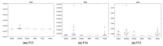
Figure 3.
Box line diagram for five algorithms on 15 benchmark functions.
Table 4.
p-values obtained from Wilcoxon Rank Sum Test for IWOA and five other algorithms.
2.3.2. Analysis of Convergence Behavior
The convergence curves of IWOA, WOA, PSO, MPA, GWO and HWOA are provided in Figure 2 to see the convergence rate of the algorithms.
From the convergence curve of Figure 2, we observe that the proposed IWOA converges significantly faster than the other five algorithms on F1–F9 and F12–F14. IWOA obtains the global optimum on F1–F4, F7, and F9. The convergence speed of HWOA is faster than WOA on most functions. Furthermore, the convergence speed of IWOA always keeps ahead of HWOA. This means that the improved strategy of WOA is more successful than HWOA. PSO has the best convergence speed and the results compare with other algorithms on F10. Although the performance of IWOA is worse than PSO on F10, IWOA still has a faster convergence speed and better results than HWOA and WOA on F10. The result of F10 shows that WOA still has limitations on the multimodal benchmark function. However, the improvement strategies help IWOA to enhance the ability of WOA to jump out of the local optimum on the multimodal benchmark function. The convergence curve of IWOA proves that the ability of IWOA to jump out of the local optimum is effectively enhanced compared to other algorithms on most benchmark functions. Therefore, the IWOA algorithm has a more vital ability to jump out of the local optimum than the other five algorithms.
2.3.3. Analysis of Exploitation Capability
Table 3 shows the optimization results of 15 benchmark functions. The proposed IWOA algorithm gives the best results of 15 benchmark functions. It can be seen that the IWOA algorithm is significantly better than the other five algorithms in terms of the mean and standard deviation of the optimum solution.
Functions F1–F5 are unimodal functions, and they have only one global optimum. The result of Table 3 shows that the IWOA is very competitive compared to the other five algorithms. Functions F6–F10 evaluate the exploration capability of an optimization algorithm. The result shows that the IWOA is better than the other five algorithms, except for F10. Functions F11–F15 are fixed-dimension multimodal functions. IWOA provides the best result on F11, F13, F14, and F15. IWOA is still competitive in F12 compared with HWOA and WOA.
Combining the results of Section 2.3.2 and Section 2.3.3 shows that the IWOA outperforms the other five algorithms in convergence speed, exploitation capability, and exploration capability on most functions.
2.3.4. Algorithmic Stability Analysis
To more visually show the stability of IWOA compared with another algorithm, we use a box line diagram to show each algorithm’s result on different functions after 30 independent runs. Figure 3 shows the result of the box line diagram.
From Figure 3, it can be seen that IWOA is more stable than other algorithms on F1, F2, F3, F4, F6, F7, F8, F9, F10, F11 and F13. Although IWOA is less stable than MPA on F12, F14, and F15, the average fitness of IWOA on F12, F14, and F15 is better than MPA. Overall, IWOA has more stability and better performance than the other algorithms on most functions.
2.3.5. Wilcoxon Rank Sum Test Analysis
In this section, we use a statistical test to evaluate the performance of IWOA in comparison with other algorithms because too many factors will influence the result of the meta-heuristics algorithm. The most common test is the Wilcoxon Rank Sum Test [38]. In the Wilcoxon Rank Sum Test, the value of the p-value is used as the evaluation criteria. Suppose the p-value is greater than 5%; in that case, it means that IWOA is not statistically different on this function compared with other algorithms. If the p-value is equal to NAN, it means that both algorithms achieve a global optimum. The result of the Wilcoxon Rank Sum Test is shown in Table 4.
In Table 4, it can be seen that HOWA and IWOA have no statistical difference on F1, F2, F3, F4, F7, F8, and F9 because they all achieve the theoretical global optimum. IWOA and WOA have the result of NAN on F9 because they achieve the theoretical optimum. IWOA and GWO have no statistical difference on F9 and F12. IWOA and MPA have the result of NAN on F7 and F9. In general, the Wilcoxon Rank Sum Test results show that IWOA is statistically different from the other five algorithms on most benchmark functions. This means that IWOA has better exploitation and exploration capability compared with the other algorithms.
3. The Principle of Semi-Supervised Support Vector Machine
Semi-Supervised Support Vector Machine
The most prominent representative of semi-supervised support vector machines (S3VM) is the Transductive Support Vector Machine (TSVM) [39]. In this paper, TSVM was introduced as S3VM. The key concept is to find appropriate mark assignments for unlabeled samples to optimize the interval after the hyperplane division. S3VM uses a local search technique to solve the problem iteratively. The detail of S3VM is in using a labeled sample collection to train an initial SVM, then using the learner to mark unlabeled samples so that all samples are labeled; based on these labeled samples, the SVM is retrained and then it searches for continuous adjustment of error-prone samples until all unlabeled samples are marked.
S3VM is also a learning method for the two-class problem, just like the regular SVM. S3VM tries to consider different potential unlabeled sample label assignments, such as trying to treat each unlabeled sample as a positive or negative example, and then looking for a dividing hyperplane in all of these results that maximizes the spacing on all samples (including labeled samples and marking the assigned unlabeled sample). Once the divisional hyper-plane is calculated, the unlabeled sample’s final marker designation is its labels [40].
There are labeled data
and
unlabeled data
,
and ,
,
. The purpose of S3VM is to predict the label
of
, ,
.
The equation of S3VM is as follows:
where
is
determined as a divide plane,
is
the slack variable,
and
are trade-off control parameters, the kernel function of S3VM is radial basis kernel function (RBF),
. Kernel parameters
and regularization
parameters C are the parameters of RBF.
4. S3VM Model Combine with Improved WOA
4.1. IWOA–S3VM Model
In Section 2, we improved WOA with the catfish effect and the adaptive cloud strategy. The results of IWOA showed that the improvement strategy was successful. We explained the basic idea of S3VM in Section 3. Since the kernel parameters of S3VM need to be specified artificially, but the kernel parameters’ values affect the classification accuracy of S3VM, we use IWOA to optimize the kernel parameter selection of S3VM. The pseudo code of IWOA–S3VM are shown in Algorithm 2.
| Algorithm 2: IWOA–S3VM. |
| Input: labeled dataset Unlabeled dataset Trade-off control parameters and Output: Predict result of Unlabeled sample: Final model of IWOA–S3VM Procedure: 1. Train model by when using IWOA to get the kernel parameters and regularization parameters C of SVM. 2. Using to predict the , get 3. Initialization 4. While do 5. To solve formula (2) with , , , and to get 6. While do 7. Based on , , , and to solve formula (17) to get 8. End while 9. End while. 10. End. |
4.2. Experiment and Result Analysis of IWOA-S3VM
In order to test the classification effect of the algorithm, it chooses five representative UCI datasets with which to run the experiment. Details of these datasets are shown in Table 5. In the experiment, firstly, each dataset is randomly divided into two parts. As shown below in Table 5, one of the total number of samples are used as the test set T. The remaining part of the data is training set L.
Table 5.
Detail of UCI datasets.
In this part, we choose SVM and S3VM compared with IWOA–S3VM; the labeled sample L was 30% and 40% of the total training set. The results are shown in Table 6 and Table 7.
Table 6.
Testing results when using 30% of training set as labeled data.
Table 7.
Testing results when using 40% of training set as labeled data.
Table 6 and Table 7 show that our algorithm has better classification accuracy than the other two algorithms. It means that the intelligent algorithm can improve the S3VM model classification accuracy. The result also shows that the accuracy of the IWOA–S3VM model will increase with the increase in labeled samples.
5. Oil Layer Recognition Application with IWOA–S3VM
5.1. Design Model of Oil Layer Recognition
A block diagram of the oil layer recognition model system based on IWOA–S3VM is shown in Figure 4. The primary step of the oil layer recognition system is shown below.

Figure 4.
Diagram of oil layer recognition model.
- (1)
- Sample information collection and pre-possessing: Due to the vast volume of logging information, it is necessary to pick sample information. The data directly connected to the oil layer details will be chosen, and the data will be separated randomly into the training dataset and the evaluation dataset. In order to prevent saturation of the measurement, all data will be normalized.
- (2)
- Attribute generalization: We set the judgment attribute in this step = {}, (1 represent oil layer).
- (3)
- Attribute reduction: In the well-logging data, there are typically at least ten kinds of well-logging information, but in most of the data, there are redundant and unnecessary attributes. In this article, we use the rough set [41] to reduce the attribute.
- (4)
- IWOA–S3VM model: Train the IWOA–S3VM model by inputting the oil layer data.
- (5)
- Output the IWOA–S3VM oil layer recognition model output when inputting the entire oil layer test results.
5.2. Practical Applications
In this section, we are using two wells of actual oil layer datasets (W1 and W2) to test the performance of the IWOA–S3VM model. The detailed information of the two oil layers is shown in Table 8. Table 9 shows the original attribution and reduction attribution of two oil layer datasets. Figure 5 shows details of the normalized attributes of W2.
Table 8.
Oil Layer dataset.
Table 9.
Attribute reduction of oil layer dataset.

Figure 5.
The normalized attributes of W2.
We used RMSE and MAE as additional performance metrics to evaluate the effectiveness of the IWOA–S3VM model. The equation is shown below:
where is the predicted value and
is the actual value.
RMSE reflects the deviation between the predicted value and the true value. MAE reflects the average value of absolute errors. Smaller values of MAE and RMSE represent the better model performance.
To test the performance of the proposed IWOA–S3VM model on semi-supervised tasks, we used 30% of the labeled data of training datasets to train the classification model. We set the maximum iteration time of IWOA as 100 times. The classification result is shown in Table 10.
Table 10.
Result of experiment.
5.3. Result of Oil Layer Recognition
Table 10 shows that the intelligent algorithm can increase the S3VM model’s accuracy. Compared to the other two algorithms, the IWOA–S3VM has better accuracy on W1 and W2. However, IWOA–S3VM uses more time compared with S3VM and SVM. The reason why IWOA takes more time is because IWOA requires several iterations to find the suitable optimization parameters of the S3VM.
In oil layer recognition, IWOA–S3VM can cope with large numbers of unlabeled datasets. The result of Table 10 shows that the S3VM model can be improved successfully by IWOA.
The actual oil layer distribution and oil layer distribution observed by the IWOA–S3VM model with the S3VM model are shown in Figure 6. The result in Figure 6 shows that the IWOA–S3VM model can more easily identify the oil layer distribution correctly when there is a quantity of unlabeled data in the oil layer datasets.

Figure 6.
Oil layer distribution of two wells by S3VM and IWOA–S3VM models.
6. Conclusions
In this paper, we proposed an IWOA–S3VM model to better utilize a large number of unlabeled samples from oil layer datasets for oil layer recognition. Firstly, IWOA is proposed to address the problems of WOA, which include getting easily trapped in the local optimum, and low convergence accuracy. We used two strategies to improve the performance of WOA; one is to use the adaptive cloud strategy to improve the global search ability of WOA, and the second is to use the catfish effect to help the WOA to jump out of the local optimum and maintain population diversity. Among the 15 benchmark functions, IWOA shows superiority over the other five algorithms. Secondly, to address the problem that the selection of kernel parameters in S3VM affects its classification accuracy, we use IWOA to optimize the selection of its kernel parameters. The classification results of the five UCI datasets show the superiority of the IWOA–S3VM model. Finally, the oil layer identification results show that IWOA–S3VM performs better than the other two algorithms when using a small number of labeled data. For future works, we will try to use other semi-supervised classification models for oil layer identification.
Author Contributions
Conceptualization, Y.P. and K.X.; methodology, Y.P. and K.X.; software, Y.P.; validation, Y.P., L.W. and Z.H.; formal analysis, Y.P. and K.X.; investigation, Y.P. and K.X.; resources, Y.P., L.W. and Z.H.; data curation, Y.P., L.W. and Z.H.; writing—original draft preparation, Y.P.; writing—review and editing, L.W. and Z.H.; visualization, L.W. and Z.H. supervision, K.X. All authors have read and agreed to the published version of the manuscript.
Funding
This work was supported by the National Natural Science Foundation of China (No. U1813222, No.42075129), Tianjin Natural Science Foundation (No.18JCYBJC16500) and Key Research and Development Project from Hebei Province (No.19210404D, No.20351802D).
Data Availability Statement
In this paper, all data generation information is given in detail in the related chapter.
Conflicts of Interest
The authors declare no conflict of interest.
References
- Hu, W.R.; Bao, W.J. Development trends of oil industry and China's countermeasures. J. China Univ. Pet. (Ed. Nat. Sci.) 2018, 42, 1–10. [Google Scholar]
- Lai, J.; Han, N.R.; Jia, Y. Detailed description of the sedimentary reservoir of a braided delta based on well logs. Geol. China 2018, 45, 304–318. [Google Scholar]
- Ellis: Well Logging for Earth Scientists; Springer: Dordrecht, The Netherlands, 2007.
- Chapelle, O.; Schölkopf, B.; Zien, A. Semi-Supervised Learning; MIT Press: Cambridge, UK, 2006. [Google Scholar]
- Chapelle, O.; Zien, A. Semi-supervised learning by low density separation. In Proceedings of the10th Information Workshop on Artificial Intelligence and Statistics, Savannah, Barbados, 6–8 January 2005; pp. 57–64. [Google Scholar]
- Ding, S.; Zhu, Z.; Zhang, X. An overview on semi-supervised support vector machine. Neural Comput. Appl. 2017, 28, 969–978. [Google Scholar] [CrossRef]
- Cheng, S.; YuHui, S.; Qin, Q. Particle warm optimization based semi-supervised learning on Chinese text categorization. In Proceedings of the 2012 IEEE Congress on Evolutionary Computation (CEC 2012), Brisbane, QLD, Australia, 10–15 June 2012; pp. 1–8. [Google Scholar]
- Zhang, T.; Xu, C.; Zhu, G. A generic framework for video annotation via semi-super- vised learning. IEEE Trans. Multimed. 2012, 14, 1206–1219. [Google Scholar] [CrossRef]
- Guilaumin, M.; Verbeek, J.; Schmid, C. Multimodal semi-supervised learning for image classification. In Proceedings of the IEEE Conference on Computer Vision and Pattern Recognition, San Francisco, CA, USA, 13–18 June 2010; pp. 902–909. [Google Scholar]
- Dan, Z.; Licheng, J.; Xue, B. A robust semi-supervised SVM via ensemble learning. Appl. Soft Comput. J. 2018, 65, 632–643. [Google Scholar]
- Zhou, Z.-H.; Li, M. Semi-supervised learning by disagreement. Knowl. Inf. Syst. 2009, 24, 415–439. [Google Scholar] [CrossRef]
- Sang, N.; Gan, H.; Fan, Y.; Wu, W.; Yang, Z. Adaptive safety degree-based safe semi-supervised learning. Int. J. Mach. Learn. Cybern. 2018, 10, 1101–1108. [Google Scholar] [CrossRef]
- Smets, P.; Kennes, R. The transferable belief model. Artif. Intell. 1994, 66, 191–234. [Google Scholar] [CrossRef]
- Mirjalili, S.; Mirjalili, S.M.; Lewis, A. Grey wolf optimization. Adv. Eng. Softw. 2014, 69, 46–61. [Google Scholar] [CrossRef]
- Faramarzi, A.; Heidarinejad, M.; Mirjalili, S. Marine Predators Algorithm: A Nature-inspired Meta heuristic. Expert Syst. Appl. 2020, 152, 113377. [Google Scholar] [CrossRef]
- Mirjalili, S.; Lewis, A. The Whale Optimization Algorithm. Adv. Eng. Softw. 2016, 95, 51–67. [Google Scholar] [CrossRef]
- Hasanien, H.M. Performance improvement of photovoltaic power systems using an optimal control strategy based on whale optimization algorithm. Electr. Power Syst. Res. 2018, 157, 168–176. [Google Scholar] [CrossRef]
- Mousavirad, S.J.; Ebrahimpour, K.H. Multilevel image thresholding using entropy of histogram and recently developed population-based metaheuristic algorithms. Evol. Intel. 2017, 10, 45–75. [Google Scholar] [CrossRef]
- Nguyen, H.; Bui, X.N.; Choi, Y. A Novel Combination of Whale Optimization Algorithm and Support Vector Machine with Different Kernel Functions for Prediction of Blasting-Induced Fly-Rock in Quarry Mines. Nat. Resour. Res. 2021, 30, 1–17. [Google Scholar] [CrossRef]
- El Aziz, M.A.; Ewees, A.A.; Hassanien, A.E. Whale Optimization Algorithm and Moth-Flame Optimization for multilevel thresholding image segmentation. Expert Syst. Appl. 2017, 83, 242–256. [Google Scholar] [CrossRef]
- Luo, J.; Shi, B. A hybrid whale optimization algorithm based on modified differential evolution for global optimization problems. Appl. Intell. 2018, 49, 1982–2000. [Google Scholar] [CrossRef]
- Hardi, M.M.; Shahla, U. A Systematic and Meta-Analysis Survey of Whale Optimization Algorithm. Comput. Intell. Neurosci. 2019, 2019, 25. [Google Scholar]
- Korashy, A.; Kamel, S.; Jurado, F.; Youssef, A.-R. Hybrid Whale Optimization Algorithm and Grey Wolf Optimizer Algorithm for Optimal Coordination of Direction Overcurrent Relays. Electr. Power Compon. Syst. 2019, 47, 644–658. [Google Scholar] [CrossRef]
- Hra, A.; Bh, A.; As, B. Optimization model for integrated river basin management with the hybrid WOAPSO algorithm. J. Hydro Environ. Res. 2019, 25, 61–74. [Google Scholar]
- Selim, A.; Kamel, S.; Jurado, F. Voltage Profile Improvement in Active Distribution Networks Using Hybrid WOA-SCA Optimization Algorithm. In Proceedings of the Twentieth International Middle East Power Systems Conference (MEPCON), Cairo, Egypt, 18–20 December 2018. [Google Scholar]
- Ye, X.; Liu, W.; Li, H.; Wang, M.; Chi, C.; Liang, G.; Chen, H.; Huang, H. Modified Whale Optimization Algorithm for Solar Cell and PV Module Parameter Identification. Complexity 2021, 2021, 1–23. [Google Scholar] [CrossRef]
- Fan, Q.; Chen, Z.; Li, Z.; Xia, Z.; Yu, J.; Wang, D. A new improved whale optimization algorithm with joint search mechanisms for high-dimensional global optimization problems. Eng. Comput. 2020, 1, 1–28. [Google Scholar] [CrossRef]
- Zhang, Q.; Liu, L. Whale Optimization Algorithm Based on Lamarckian Learning for Global Optimization Problems. IEEE Access 2019, 7, 36642–36666. [Google Scholar] [CrossRef]
- Chen, X. Research on New Adaptive Whale Algorithm. IEEE Access 2020, 8, 90165–90201. [Google Scholar] [CrossRef]
- Wolpert, D.H.; Macready, W.G. No free lunch theorems for optimization. IEEE Trans. Evol. Comput. 1997, 1, 67–82. [Google Scholar] [CrossRef]
- Pan, Y.-K.; Xia, K.-W.; Niu, W.-J.; He, Z.-P. Semisupervised SVM by Hybrid Whale Optimization Algorithm and Its Application in Oil Layer Recognition. Math. Probl. Eng. 2021, 2021, 1–19. [Google Scholar] [CrossRef]
- Xu, H.Y.; Tian, Y.B.; Huang, T.A. Cloud Adaptive Particle Swarm Optimization Algorithm Based on Cloud Variation. Comput. Simul. 2012, 11, 251–255. [Google Scholar]
- Sabharwal, A.; Selman, S.; Russell, B. Artificial intelligence: A modern approach, third edition. Artif. Intell. 2011, 175, 935–937. [Google Scholar] [CrossRef]
- Xu, G.; Yu, L.; Guo, J. Application of Optimization Algorithm on Cloud Adaptive Gradient Particle Swarm Optimization in Optimum Reactive Power. J. Comput. Inf. Syst. 2011, 7, 57–72. [Google Scholar]
- Chuang, L.Y.; Tsai, S.W.; Yang, C.H. Catfish particle swarm optimization. In Proceedings of the IEEE Swarm Intelligence Symposium (SIS ’08), St. Louis, Mo, USA, 21–23 September 2008. [Google Scholar]
- Gharehchopogh, F.S.; Gholizadeh, H. A comprehensive survey: Whale optimization algorithm and its applications. Swarm Evol. Comput. 2019, 48, 1–24. [Google Scholar] [CrossRef]
- Suganthan, P.N.; Hansen, N.; Liang, J. Problem Definitions and Evaluation Criteria for the CEC 2005 Special Session on Real-Parameter Optimization. Nat. Comput. 2005, 2005, 341–357. [Google Scholar]
- Derrac, J.; García, S.; Molina, D.; Herrera, F. A Practical Tutorial on the Use of Nonparametric Statistical Tests as a Methodology for Comparing Evolutionary and Swarm Intelligence Algorithms. Swarm Evol. Comput. 2011, 1, 3–18. [Google Scholar] [CrossRef]
- Joachims, T. Transudative inference for text classification using support vector machines. In Proceedings of the 16th International Conference on Machine Learning; Morgan Kaufmann Publishers Inc.: San Fran-cisco, CA, USA, 1999; pp. 200–209. [Google Scholar]
- Fu, Y.; Wang, X. Radar Signal Recognition Based on Modified Semi-Supervised SVM Algorithm. In Proceedings of the IEEE 2nd Advanced Information Technology, Electronic and Automation Control Conference (IAEAC 2017), Chongqing, China, 25–26 March 2017; pp. 2392–2396. [Google Scholar]
- Bai, J.; Xia, K.; Lin, Y.; Wu, P. Attribute Reduction Based on Consistent Covering Rough Set and Its Application. Complexity 2017, 2017, 1–9. [Google Scholar] [CrossRef]
Publisher’s Note: MDPI stays neutral with regard to jurisdictional claims in published maps and institutional affiliations. |
© 2021 by the authors. Licensee MDPI, Basel, Switzerland. This article is an open access article distributed under the terms and conditions of the Creative Commons Attribution (CC BY) license (https://creativecommons.org/licenses/by/4.0/).