Quasi-Rational Analytic Approximation for the Modified Bessel Function I₁(x) with High Accuracy

Abstract

A new simple and accurate expression to approximate the modified Bessel function of the first kind $I_1(x)$ is presented in this work. This new approximation is obtained as an improvement of the multi-point quasi-rational approximation technique, MPQA. This method uses the power series of the Bessel function, its asymptotic expansion, and a process of optimization to fit the parameters of a fitting function. The fitting expression is formed by elementary functions combined with rational ones. In the present work, a sum of hyperbolic functions was selected as elementary functions to capture the first two terms of the asymptotic expansion of $I_1(x)$, which represents an important improvement with respect to previous research, where just the leading term of the asymptotic series was captured. The new approximation function presents a remarkable agreement with the analytical solution $I_1(x)$, decreasing the maximum relative error in more than one order of magnitude with respect to previous similar expressions. Concretely, the relative error was reduced from ${10}^{-2}$ to $4\times {10}^{-4}$, opening the possibility of applying the new improved method to other Bessel functions. It is also remarkable that the new approximation is valid for all positive and negative values of the argument.

1. Introduction

The Bessel equation and its modified form play an important role for modeling common problems in science and engineering. These equations appear in different contexts spanning areas like electrodynamics [1,2], plasma-physics [3,4,5], heat transfer [6,7,8], chemical engineering [9], fluid mechanics [10,11], and others [12,13]. Bessel functions with integer order appear in systems with cylindrical symmetry, and those with half integer order in spherical symmetries. The first kind solution of the modified Bessel equation is called $I_{\nu }(x)$, and it corresponds to a power series which is used to obtain the solution of a variety of problems. However, the numerical calculation for large and intermediate values of x requires a large number of terms of the series to get good accuracy, which has impulsed a range of different techniques for computing the modified Bessel functions properly in a reasonable time frame. In general, these techniques pursue two kinds of goals. A first group focuses on formulating a simple approximation of the modified Bessel function with a low number of fitting parameters. They can be used in correlations originated from the Bessel equation or from more complex equations where the Bessel equation is involved. These approximations allow a simple and direct computation of the solution, without using the modified Bessel function itself. An example of this kind of technique is the model proposed in [14], where the modified Bessel function is approximated by a finite sum of exponential functions, which considers eight fitting parameters established for different intervals of the domain. A more extensive analytic approximation for the specific case of $I_1(x)$ has also been published in [15]. The method to obtain this approximation was based on the so-called multi-point quasi-rational approximation technique (MPQA) [16]. That approximation is valid for any positive value of x, and its maximum relative error was about one percent, considering just five parameters for the entire domain.

On the other hand, there is a second group of approximation techniques focused exclusively on the accuracy of the fitting function, which implies a larger number of fitting parameters, truncated series, or algorithms based on conditional loops. In this case, the Bessel approximation can be coded in a programming language to be used in computers as a function that can be easily called by a user. An important initial attempt to achieve a high level of accuracy was made by polynomial approximations in [17], and it was coded in different programming languages [18]. Here, eight or ten fitting parameters are used in an expression for $I_1(x)$, depending on the argument interval. The fitting function resembles the power series and the asymptotic expansion of the modified Bessel function, for low and large values of the argument, respectively. A simple method in this group considers to compute the power series and the asymptotic expansion of the modified Bessel function directly, defining a criterion for limiting the scope of each series and the number of terms to be used. This was proposed in [19], where a code written in FORTRAN language is presented for computing $I_{\nu }(x)$. A remarkable fast technique to compute the modified Bessel function with a high level of precision is presented in [20]. This technique is based on an algorithm that evaluates the ratio of the $(k+1)$st term to the kth term of the power series of $I_{\nu }(x)$ in a loop. The iterative code is very simple and short, and surprisingly faster than some well-established software like MATHEMATICA and MAPLE in several orders of magnitude for large arguments, which was verified in the same work by running time experiments made in a common laptop.

In the present work, a simple and very precise analytic approximation for $I_1(x)$ has been determined using only six fitting parameters. The methodology corresponds to the MPQA as in [15], but the structure of the new approach differs substantively from the previous one. Now, the new structure is built in such a way that includes more information from the asymptotic expansion of $I_1(x)$. Specifically, a sum of two hyperbolic functions (combined with rational ones) was introduced. The direct effect of this change on the new approach was the capture of the two first leading terms of the asymptotic expansion, producing a strong increment in accuracy for intermediate values of the x variable. The new approximation is valid for any real value of x, positive or negative.

The theoretical treatment of this study, including the equations to determine the fitting parameters of the analytic approximation of $I_1(x)$, will be presented in Section 2. The results and discussion will be performed in Section 3. An analysis to determine the convergence of the new approximation to the exact function has also been included at the end of Section 3. Finally, Section 4 will be devoted to the conclusions of this work.

2. Theoretical Treatment

The general procedure to find an approximate expression for the modified Bessel function consists of: (a) selecting a suitable structure for a fitting function; (b) to establish the constraints on the fitting parameters; (c) to write these parameters as a function of just one parameter, which is taken as an independent variable; and (d) to optimize the fitting parameters minimizing the error.

2.1. Fitting Function

The modified Bessel function of order $\nu$ and its asymptotic expansion are some well known series [17]; they are given respectively by:

$$\begin{array}{ccc}\hfill I_{\nu }(x)& =& \sum _{k=0}^{\infty }\frac{1}{k!\Gamma (k+\nu +1)}{\left(\frac{x}{2}\right)}^{2k+\nu }\hfill \end{array}$$

(1)

$$\begin{array}{ccc}\hfill I_{\nu }(x)& \sim & \frac{e^x}{\sqrt{2\pi x}}\left(1-\frac{4{\nu }^2-1}{8x}+\frac{(4{\nu }^2-1)(4{\nu }^2-9)}{2!{(8x)}^2}-...\right).\hfill \end{array}$$

(2)

If $\nu$ is a positive integer, the Gamma function $\Gamma$ can be evaluated by using the rule: $\Gamma (n+1)=n!$. Specifically, for $\nu =1$, the following series are obtained:

$$\begin{array}{ccc}\hfill I_1(x)& =& \frac{x}{2}\left(1+\frac{x^2}{8}+\frac{x^4}{192}+...\right)\hfill \end{array}$$

(3)

$$\begin{array}{ccc}\hfill I_1(x)& \sim & \frac{e^x}{\sqrt{2\pi x}}\left(1-\frac{3}{8x}-\frac{15}{128x^2}-...\right).\hfill \end{array}$$

(4)

An interesting challenge is given by building a fitting function that captures the behavior of the modified Bessel series for small values of x, and the behavior of the asymptotic expansion for large values of x. The complexity for the conciliation of these limiting behaviors is rooted in the fact that the modified Bessel series is formed by even powers, while its expansion has inverse powers of x and also a prefactor $e^x/\sqrt{x}$. A simple option to achieve this corresponds to the following approximation function:

$${\tilde{I}}_1(x)=\frac{(p_0+p_2{x}^2)sinh(x)+x(p_1+p_3{x}^2)cosh(x)}{2{(1+{\lambda }^4{x}^2)}^{3/4}(1+q{x}^2)},$$

(5)

where $\lambda$, $p_0$, $p_1$, $p_2$, $p_3$, and q correspond to fitting parameters. The function ${\tilde{I}}_1(x)$ captures the prefactor $e^x/\sqrt{x}$ and the first two terms of the asymptotic expansion for big values of x through: (1) the exponential behavior of $sinh(x)$ and $cosh(x)$, and (2) the limits of the different components of ${\tilde{I}}_1(x)$ when $x\to \infty$. At the same time, this analytic approximation can be equalized for small values of x with the first tree terms of the modified Bessel function, as it will be described in the next sub-section. The parameter $\lambda$ constitutes the optimization variable, which means that all the others parameters depend on $\lambda$ for this purpose. Thus, $\lambda$ will vary freely to find the optimal fitting function ${\tilde{I}}_1(x)$ for which the error will be minimized.

The approximation function shown in Equation (5) also allows for being expanded to capture more terms of the asymptotic series of $I_1(x)$. Indeed, including successive sums of the hyperbolic functions $sinh(x)$ and $cosh(x)$ multiplied by suitable polynomial fractions, it is possible to capture more terms of Equation (4) for large values of the argument x.

It is important to point out some features of ${\tilde{I}}_1(x)$. A remarkable characteristic of the function ${\tilde{I}}_1(x)$ is that it is an odd function. The power series shows this symmetry, but this characteristic is broken for the asymptotic expansion. The new function ${\tilde{I}}_1(x)$ keeps the symmetry of the power series and also represents two terms of the asymptotic expansion without breaking this symmetry. This is done by obtaining the exponential behavior of expansion by means of $xcoshx$ and $sinhx$. In the previous work presented in [15], this symmetry is also kept, but only the leading term of the asymptotic expansion is captured. In the present work, the leading term and the next one are used, but additionally more asymptotic terms can be incorporated by increasing the number of even powers in the numerator and denominator.

2.2. Fitting Parameters

The fitting parameters will be subjected to different constraints to mimic the behavior of the modified Bessel function $I_1(x)$ and its corresponding asymptotic expansion. In addition, a condition to guarantee continuity by avoiding singularities will be imposed.

2.2.1. Constraints for Large Values of x

By equating the first two terms of the Equation (4) with the approximation function given in (5) for high values of the variable x, we arrive to:

$$\begin{array}{ccc}\hfill \frac{e^x}{4}·\frac{p_2+p_{3}x}{{\lambda }^{3}q{x}^{3/2}}& =& \frac{e^x}{\sqrt{2\pi x}}\left(1-\frac{3}{8x}\right).\hfill \end{array}$$

(6)

The following expressions are obtained from Equation (6):

$$\begin{array}{ccc}\hfill p_2& =& -\frac{3}{4}\sqrt{2/\pi }{\lambda }^{3}q\hfill \end{array}$$

(7)

$$\begin{array}{ccc}\hfill p_3& =& 2\sqrt{2/\pi }{\lambda }^{3}q.\hfill \end{array}$$

(8)

It is important to emphasize that $p_2$ is coming from $sinhx$ and $p_3$ from $coshx$. If only one hyperbolic function is used, then only the information coming from the leading term of the asymptotic expansion is considered. To introduce the information from two consecutive terms of the asymptotic expansion, two hyperbolic functions have to be used.

2.2.2. Constraints for Low Values of x

For small values of x, it is possible to use the Taylor series around $x=0$ to approximate the expressions contained in ${\tilde{I}}_1(x)$; this is:

$$\begin{array}{ccc}\hfill sinh(x)& \approx & x\left(1+\frac{x^2}{6}+\frac{x^4}{120}\right)\hfill \end{array}$$

(9)

$$\begin{array}{ccc}\hfill cosh(x)& \approx & 1+\frac{x^2}{2}+\frac{x^4}{24}\hfill \end{array}$$

(10)

$$\begin{array}{ccc}\hfill {(1+{\lambda }^4{x}^2)}^{3/4}& \approx & 1+\frac{3}{4}{\lambda }^4{x}^2-\frac{3}{32}{\lambda }^8{x}^4.\hfill \end{array}$$

(11)

Using the Equations (9)–(11), and then matching the approximation function ${\tilde{I}}_1(x)$ with the first two terms of the Bessel series, the following polynomial equation is obtained:

$$\begin{array}{ccc}\hfill (p_0+p_2{x}^2)\left(1+\frac{x^2}{6}+\frac{x^4}{120}\right)+(p_1+p_3{x}^2)\left(1+\frac{x^2}{2}+\frac{x^4}{24}\right)& =& \\ \hfill \left(1+\frac{x^2}{8}+\frac{x^4}{192}\right)\left(1+\frac{3}{4}{\lambda }^4{x}^2-\frac{3}{32}{\lambda }^8{x}^4\right)(1+q{x}^2).\end{array}$$

(12)

Truncating the terms of degree 6 or bigger in Equation (12) and equating the polynomial coefficients, it is relatively straightforward to arrive to the following equation system:

$$\begin{array}{ccc}\hfill p_0+p_1& =& 1\hfill \end{array}$$

(13)

$$\begin{array}{ccc}\hfill \frac{p_0}{6}+\frac{p_1}{2}+p_2+p_3& =& \frac{1}{8}+\frac{3}{4}{\lambda }^4+q\hfill \end{array}$$

(14)

$$\begin{array}{ccc}\hfill \frac{p_0}{120}+\frac{p_1}{24}+\frac{p_2}{6}+\frac{p_3}{2}& =& \frac{1}{192}+\frac{3}{32}{\lambda }^4(1-{\lambda }^4)+\left(\frac{1}{8}+\frac{3}{4}{\lambda }^4\right)q.\hfill \end{array}$$

(15)

The equation system for the fitting parameters obtained before can by solved by adding Equations (7) and (8) from the analysis for large values of x. As we said before, the parameter $\lambda$ will be a free parameter, and then all the rest of parameters will be a function of $\lambda$.

2.2.3. Non-Zero Point Constraint

An important requirement for ${\tilde{I}}_1(x)$ corresponds to avoid artificial zero values in the denominator, which are called defects according to the well known Padé Approximant technique. These points can be removed by restricting q to a positive value. The expression for q corresponds to:

$$\begin{array}{ccc}\hfill q& =& \frac{1+18{\lambda }^4-90{\lambda }^8}{24\left(-1+30\sqrt{2/\pi }{\lambda }^3-30{\lambda }^4\right)},\hfill \end{array}$$

(16)

where $\lambda$ is considered to be positive. Figure 1 shows the parameter q as a function of $\lambda$. Note that q is positive between the two vertical asymptotes and for values of $\lambda$ located a little after the asymptote placed in $\lambda =0.7$. In addition, note that all q values that are positive are suitable to use, but values of q (and $\lambda$) very close to a vertical asymptote should be determined considering many significant figures due to the big slope in these zones. In the present work, we consider a limit of four significant figures for all the parameters to keep the simplicity of the fitting function.

3. Results and Discussion

The criterion for determining $\lambda$ is by comparing the maximum relative error of the fitting function for different $\lambda$ values. In this sense, two kinds of error definitions were established: (1) an error in a point x given the $\lambda$ value ${\epsilon }_p(x,\lambda )$, and (2) a global error $\epsilon (\lambda )$ evaluated on an interval $[a,b]$ of the x variable. This last error is given by the maximum error ${\epsilon }_p(x,\lambda )$ in the interval $[a,b]$. The expressions for the error (1) and (2) are:

$$\begin{array}{ccc}\hfill {\epsilon }_p(x,\lambda )& =& \frac{|I_1(x)-{\tilde{I}}_1(x,\lambda )|}{I_1(x)}\hfill \end{array}$$

(17)

$$\begin{array}{ccc}\hfill \epsilon (\lambda )& =& max{\left[{\epsilon }_p(x,\lambda )\right]}_{x\in [a,b]}.\hfill \end{array}$$

(18)

Figure 2 shows the error $\epsilon$ in the interval $x\in [0,500]$ as a function of $\lambda$. In Figure 2a, four local minimum points of the $\epsilon (\lambda )$ function can be localized. Figure 2b zooms in the zone where the absolute minimum value of the error is located. This absolute minimum value called ${\epsilon }^{min}$ corresponds to $0.0003938$, and it occurs for ${\lambda }^{min}=0.4800$. Note that, when $\lambda ={\lambda }^{min}$, the value of the parameter q corresponds to $1.297$, which satisfied the non-singular point constraint. Then, the optimal values of each parameter of the fitting function can be determined, and they are the ones shown in

Table 1. Optimal values of the fitting parameters for the analytic fitting function ${\tilde{I}}_1(x)$.

$\mathit{\lambda }$	q	${\mathit{p}}_0$	${\mathit{p}}_1$	${\mathit{p}}_2$	${\mathit{p}}_3$
0.4800	1.297	−2.457	3.457	−0.08585	0.2289

.

Using the values from Table 1, the analytic fitting function is expressed as:

$${\tilde{I}}_1(x)=\frac{(-2.457-0.08585x^2)sinh(x)+x(3.457+0.2289x^2)cosh(x)}{2{(1+0.{4800}^4{x}^2)}^{3/4}(1+1.297x^2)}.$$

(19)

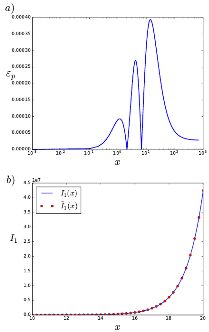
Figure 3a shows the relative error of the fitting function ${\tilde{I}}_1(x)$ (Equation (19)). The maximum error, which also corresponds to ${\epsilon }^{min}$, is $0.0004$ or $0.04\%$. This maximum error is reached for $x\approx 14$, and it is more than one order of magnitude lower than previous research, where the error reaches a value of 1 percent [15]. Additionally, in Figure 3b, the analytic approximation function ${\tilde{I}}_1(x)$ is shown in comparison with the actual modified Bessel function, across the zone where the error reaches its maximum value of $0.0004$. Note the strong similarity between both functions.

It is interesting to point out that the relative error of the approximation decreases with x, which shows the convergence between the approximation and the real function for large values of x. This is a consequence of the convergence between the asymptotic behaviors of the two functions. On the other side, there is also a convergence in the values near zero. The points with the higher errors will be always for intermediate x values.

It is important to note that the approximation here obtained is an odd function of x, and therefore is good for positive as well as negative values of x. To clarify more this matter, it is useful to compare the present approximation with that in Ref. [17], where two approximations have been determined, one valid for x in the interval $-3.75\le x\le 3.75$ and the second one for positive $x>3.75$. The total number of parameters to be determined there are 16, six for the first interval and ten for the second one. Now, in the present work, only one approximation has been determined valid for every value of x, positive or negative, using only six parameters. In our analysis, relative errors are analyzed instead of absolute ones because, in most of applications, the function $I_1(x)$ appears as a factor, and, for these cases, the relative error is the simplest option to be evaluated.

The approximations by finite sum of exponential functions are also important in [14]. The characteristics of these approximations are that each one is limited to an interval. Using four intervals, they obtain fitting functions for all positive values of x. However, the maximum relative error corresponds to 0.002 at x = 0, which is larger by a factor of five than the one here presented with only one function, and also valid for any positive and negative value of x.

As it has been mentioned before, there are two different goals when an approximation of the modified Bessel function is built: simplicity or extreme accuracy. Our goal was to produce a simple expression suitable for using in correlations or rapid computations with a calculator, but, at the same time, providing an excellent level of accuracy. Methods based on loops or finite series achieve in general more accuracy, but they need to be coded, and they also have a computational cost intrinsic, which is negligible for our new approximation function. The relative error in a loop routine can be of order ${10}^{-15}$, but the running time in a common two core laptop can fluctuate from a fraction of second to several minutes to compute $I_1(x)$ for large values of x, depending on the routine method [20].

To study the convergence of the present approximation ${\tilde{I}}_1(x)$ with respect to the exact function, the following analysis has been performed. First, the asymptotic behavior of ${\tilde{I}}_1(x)$ is analyzed. After that, we look for the differences with the asymptotic expansion of $I_1(x)$. Finally, the relative error ${\epsilon }_p(x)$ for large values of x is determined, showing the actual convergence of ${\epsilon }_p(x)$ for large values of x.

$$\begin{array}{ccc}\hfill {\tilde{I}}_1(x)& =& \frac{1}{4{\lambda }^{3}q\sqrt{x}{\left(1+\frac{1}{{\lambda }^4{x}^2}\right)}^{3/4}\left(1+\frac{1}{q{x}^2}\right)}\left((e^x+e^{-x})\left(p_3+\frac{p_1}{x^2}\right)+\frac{e^x-e^{-x}}{x}\left(p_2+\frac{p_0}{x^2}\right)\right)\hfill \end{array}$$

(20)

$$\begin{array}{ccc}\hfill {\epsilon }_p(x)& =& \frac{\left|I_1(x)-{\tilde{I}}_1(x)\right|}{I_1(x)}\hfill \\ \hfill & =& \frac{\left|\frac{e^x}{\sqrt{2\pi x}}\left(1-\frac{3}{8x}\right)-\frac{e^x}{4{\lambda }^{3}q\sqrt{x}}\left(p_3+\frac{p_2}{x}\right)\right|}{\frac{e^x}{\sqrt{2\pi x}}\left(1-\frac{3}{8x}\right)}+\mathcal{O}\left(\frac{1}{x^2}\right)\hfill \\ \hfill & =& \frac{\left|1-\frac{3}{8x}-\frac{\sqrt{2\pi }}{4·{0.4800}^{3}1.297}\left(0.2289-\frac{0.08585}{x}\right)\right|}{1-\frac{3}{8x}}+\mathcal{O}\left(\frac{1}{x^2}\right)\hfill \\ \hfill & =& \frac{\left|-2.8·{10}^{-5}+\frac{6.5·{10}^{-5}}{x}\right|}{1-\frac{3}{8x}}+\mathcal{O}\left(\frac{1}{x^2}\right)\hfill \\ & =& \left|-2.8·{10}^{-5}+\frac{6.5·{10}^{-5}}{x}\right|+\mathcal{O}\left(\frac{1}{x^2}\right)\hfill \end{array}$$

(21)

It is clear from this result that the relative error for large values of x will be $2.8·{10}^{-5}$, lower than the maximum relative error here found of $0.0004$. In the present approximation, all the parameters are given with four decimals since that is enough to keep the largest relative error as low as $0.0004$. The calculation we have done shows that, if the parameters are given with more digits, then the relative error for large x can be decreased, but the maximum relative error will be the same. In case that, for any reason, a researcher needs higher approximation for large values of x, the parameters given in Table 1 should be improved to obtain an error of $\mathcal{O}\left(\frac{1}{x}\right)$ or even of $\mathcal{O}\left(\frac{1}{x^2}\right)$.

4. Conclusions

A simple and accurate analytic approximation for the first kind modified Bessel function $I_1(x)$ has been determined in the present work. This approximation is much better than in a previous version [15], since the relative error is more than one order of magnitude lower than the previous one, decreasing from $1\%$ to $0.04\%$, and also lower (by a factor of five) than other method of the same category based on exponential functions. This substantial improvement is rooted in the new structure of the fitting function, which captures two terms of the asymptotic series of $I_1(x)$, instead of just one as in the previous approximation version. The structural change in the new fitting function consists of the incorporation of the sum of two hyperbolic functions weighted through rational functions, which can be extended to capture more terms of the asymptotic expansion of $I_1(x)$. An important point is that the new improvement can be applied to all Bessel functions, opening the door to new studies and perspectives. The approximation here presented is valid not only for any positive values of x, but also for negative ones. It can also be differentiated and integrated as the real $I_1(x)$, since only one fitting function is good for all the values of the argument. Furthermore, the relative error of the new approximation is about $4·{10}^{-4},$ which will be right for most of the applications. In addition, the calculation can be performed with a simple pocket calculator. Finally, one last analysis has also been performed showing the convergence of ${\tilde{I}}_1(x)$ to $I_1(x)$ for large values of x. It is clear that the relative error decreases for large values of x, and the maximum relative error is always for intermediate values of the variable x.

References

1. Jackson, J.D. Classical Electrodynamics, 3rd ed.; John Wiley & Sons: Hoboken, NJ, USA, 1998; pp. 212–219. [Google Scholar]
2. Gaete, P.; Helayel-Neto, J.; Spallucci, E. Aspects of finite electrodynamics in D = 3 dimensions. J. Phys. A Math. Theor. 2012, 45, 215401. [Google Scholar] [CrossRef] [Green Version]
3. Chen, F.F. Introduction to Plasma Physics and Controlled Fusion; Plenum Press: New York, NY, USA, 1984; Volume 1, pp. 19–51. [Google Scholar]
4. Salamin, Y.I. Fields of a Bessel-Bessel light bullet of arbitrary order in an under-dense plasma. Sci. Rep. 2018, 8, 1–8. [Google Scholar]
5. Qin, H.; Phillips, C.K.; Davidson, R.C. A new derivation of the plasma susceptibility tensor for a hot magnetized plasma without infinite sums of products of Bessel functions. Phys. Plasmas 2007, 14, 092103. [Google Scholar] [CrossRef] [Green Version]
6. Kraus, A.D.; Aziz, A.; Welty, J. Extended Surface Heat Transfer; John Wiley & Sons: Hoboken, NJ, USA, 2001; pp. 17–23. [Google Scholar]
7. Han, J.C. Analytical Heat Transfer; Taylor & Francis: Abingdon, UK, 2012; pp. 27–38. [Google Scholar]
8. Philippe, M.; Bernier, M.; Marchio, D. Validity ranges of three analytical solutions to heat transfer in the vicinity of single boreholes. Geothermics 2009, 38, 407–413. [Google Scholar] [CrossRef]
9. Varma, A.; Morbidelli, M. Mathematical Methods in Chemical Engineering; Oxford University Press: Oxford, UK, 1997; pp. 311–329. [Google Scholar]
10. Fetecau, C.; Fetecau, C.; Vieru, D. On some helical flows of Oldroyd-B fluids. Acta Mech. 2007, 189, 53–63. [Google Scholar] [CrossRef]
11. Fitt, A.D.; Gonzalez, G. Fluid mechanics of the human eye: Aqueous humour flow in the anterior chamber. Bull. Math. Biol. 2006, 68, 53. [Google Scholar] [CrossRef] [PubMed]
12. Watson, G.N. A Treatise on the Theory of Bessel Functions, 2nd ed.; Cambridge University Press: Cambridge, UK, 1966. [Google Scholar]
13. Korenev, B.G. Bessel Functions and Their Applications; Taylor and Francis: London, UK; New York, NY, USA, 2002. [Google Scholar]
14. Salahat, R.; Salahat, E.; Hakam, A.; Assaf, T. A simple and efficient approximation to the modified Bessel functions and its applications to Rician fading. In Proceedings of the 2013 7th IEEE GCC Conference and Exhibition (GCC), Doha, Qatar, 17–20 November 2013; pp. 351–354. [Google Scholar]
15. Martin, P.; Olivares, J.; Sotomayor, A. Precise analytic approximation for the modified Bessel function I1(x). Rev. Mex. Física 2017, 63, 130–133. [Google Scholar]
16. Martin, P.; Castro, E.; Paz, J.L.; De Freitas, A. Multipoint Quasi-Rational Approximants in Quantum Chemistry, Ch. 3, New Developments in Quantum Chemistry; Paz, J.L., Hernandez, A.J., Eds.; Transworld Research Network: Kerala, India, 2009; pp. 55–78. [Google Scholar]
17. Abramowitz, M.; Stegun, I.A. Handbook of Mathematical Functions, Ninth Printing; Dover Publications Inc.: Mineola, NY, USA, 1970; pp. 374–379. [Google Scholar]
18. Press, W.H.; Teukolsky, S.A.; Vetterling, W.T.; Flannery, B.P. Numerical Recipes in C; Cambridge University Press: New York, NY, USA, 2002; pp. 236–240. [Google Scholar]
19. Geelen, B.B. Accurate solution for the modified Bessel function of the first kind. Adv. Eng. Softw. 1995, 23, 105–109. [Google Scholar] [CrossRef]
20. Sra, S. A short note on parameter approximation for von Mises-Fisher distributions: A fast implementation of Is(x). Comput. Stat. 2012, 27, 177–190. [Google Scholar] [CrossRef]
Figure 1. Parameter q of the approximation function I ˜ 1 ( x ) as a function of λ . Dotted lines: vertical asymptotes.
Symmetry 13 00741 g001
Figure 2. Relative global error ε of the fitting function as a function of λ . (a) large range of λ ; (b) close up of the zone where the absolute minimum value is located.
Symmetry 13 00741 g002
Figure 3. Error of the approximation function. (a) relative error ε p for the analytic approximation given by Equation (19) as a function of x; (b) analytic approximation function I ˜ 1 ( x ) in comparison with the actual modified Bessel function I 1 ( x ) .
Symmetry 13 00741 g003