A Self-Organizing Area Coverage Method for Swarm Robots Based on Gradient and Grouping

Abstract

The openness of the environment brings great challenges to the swarm robotic system to cover the task area quickly and effectively. In this paper, a coverage method based on gradient and grouping (GGC) is proposed. What is novel about our proposed solution is that it is suitable for extremely simple robots that lack computing or storage power. Through the change of the robot gradient, the swarm robot system with very simple functions can effectively self-organize to cover the unknown task area. By grouping the swarm robots, each group can cover the task area in parallel, which greatly improves the coverage speed. We verified our proposed method through experimental simulation and found that the gradient and grouping-based method in this paper was superior to other methods in terms of coverage, coverage completion time, and other aspects. Simultaneously, the robustness of the proposed method is analyzed and admirable experimental results are obtained. Because the applicable robot is very simple, the method in this paper can be applied to the submillimeter swarm robot system, which will lay the foundation for micro medicine.

1. Introduction

Swarm robots are composed of a large number of simple agents with autonomous capabilities, local communication, and perceived energy. Through a few simple rules, the whole system can show complex swarm behavior characteristics such as self-organization and cooperation [1]. Swarm robots were inspired by the many biological species that demonstrate collective behavior in nature [2,3,4]. In this kind of collective behavior, local interactions between individuals and the environment lead to a set of independent agents in a distributed way to solve complex tasks, without the central control unit. The locality of interaction and communication between robots may be seen as a limitation, but it has a good effect on the scalability and robustness of the system and is therefore generally superior to the use of global communication and global perception.

Wireless sensor coverage can be widely used in forest monitoring [5,6], industrial monitoring [7,8], battlefield monitoring [9,10], disaster prevention [11,12], and other application fields, by deploying a large number of wireless sensors in some specific task areas to form a network to collect the data. Using large-scale swarm robots to replace sensors for regional coverage will improve the coverage rate of the area, while the robots can patrol a local area [13,14,15]. At the same time, the swarm robotic system also has better robustness and scalability for regional coverage.

The neural network (NN) method has been widely used in robot motion planning, control and coverage [16,17,18]. Luo et al. [19] proposed a neurodynamic method for multi-robot region full coverage navigation and designed a bionic neural network to build a workspace model and guide the multi-robot to complete the coverage task. The method does not need to know the environment or any predefined template in advance, and it can be completed automatically without any manual intervention, which has high computational efficiency and flexibility. However, most neural network methods are only applicable to a single robot for region coverage [20,21]. Moreover, some neural network models need to learn programs, which have a high computational cost and are difficult to achieve real-time regional coverage.

Gage [22] introduced three basic types of multi-robot system coverage: blanket coverage, barrier coverage, and sweep coverage. Blanket coverage means that enough robots can be statically covered in the whole target area. Barrier coverage is made by placing multiple robots in a barrier that can be detected when a moving robot passes through the barrier. Sweep coverage is to plan a suitable path for multiple robots at the same time and to access every part of the area by scanning.

Many researchers use different approaches to solve the problem of area coverage and pattern formation in swarm robots. Behavior-based methods and potential field methods are often used in these models [23,24,25]. Other approaches include the virtual structure strategy [26,27] and the leader-follower approach [28,29,30]. However, in all of these methods, the computational cost increases significantly with the size of the group [31].

A pattern formation method for regional formation using the robot population was proposed in [32], which can adapt to the environment change caused by unknown target movement or obstacle. However, these methods use global coordinates and need to know the shape of the region. Ozdemir et al. [33] proposed a simple method to solve the problem of collaborative coverage of unknown two-dimensional space by a group of anonymous mobile robots. This controller is suitable for robots lacking calculation or storage. However, the coverage rate and the coverage uniformity cannot be guaranteed.

Kantaros et al. [34] proposed a coverage method based on visibility awareness control, which introduced a new concave division technology, and extended the power diagram to the power diagram based on visibility. This method has achieved good results in the problem of concave surface coverage. A sensor coverage optimization algorithm based on PSO is proposed in [35], and the Voronoi diagram was used to realize the coverage of the region. An artificial bee colony algorithm and particle swarm optimization algorithm was used to solve the sensor configuration problem [36], and then the heuristic algorithm was used for scheduling. However, these methods are not suitable for complex environments and large-scale robots.Teruel et al. [37] proposed a distributed self-deployment mechanism (Centroidal Voronoi Tessellations (CVT), which enables the swarm robots to self-organize and evenly cover the dynamic region, greatly improving the convergence of the system through feedforward actions. Cortés et al. [38] proposed the coordination algorithm for mobile agent groups to perform deployment and coverage tasks, and based on the geometric properties of Voronoi partitions and adjacent graphs, a class of clustering objective functions is analyzed, and continuous-time and discrete-time covering algorithms are proposed. The convergence speed of this method is improved greatly, but it cannot adapt to a complex environment. Moreover, the deployment method based on Vornoni graphs can only solve the problem when the target region is a convex polygon.

Hsiang et al. [39] proposed a local rule based on following the leadership. When the robot is a primitive finite automaton with only local communication, local sensors and constants, the time needed to fill the whole area can be minimized. However, it cannot adapt to the dynamic environment and too much reliance on leaders, resulting in its slow convergence speed.

McLurkin et al. [40] described a set of a distributed algorithm, the algorithm uses the directional diffusion method to achieve the area coverage of swarm robots. Besides, the gradient-based routing protocol is used for remote communication, which allows the robot to explore the large and complex indoor environment. However, this method has low efficiency, and the robot has strong jitter during regional coverage, so it cannot achieve a stable coverage state.

Rubenstein et al. [41] proposed a programmable self-assembly method for large-scale robots, which can support thousands of robots to form a various complex patterns by self-organization. However, the pattern must be predefined, and the speed of coverage is very slow.

For the swarm robotic system with simple functions, it can only carry out local perception and local communication. Limited computing power and communication bandwidth make it unable to be extended to large-scale and more complex tasks. For the dynamic unknown environment, there are many challenges for swarm robots to cover the task area quickly and effectively through self-organization.

• It is very difficult to cover the unknow area effectively for the swarm robots by self-organization.
• A large number of swarm robots are needed for a large area, and the coverage may take a long time.

Given the above challenges, this paper proposes a self-organization blanket coverage method based on gradient and grouping for large-scale swarm robots, which can cover the unknown complex area effectively and quickly. The two contributions are as follows:

• Gradient generation is only carried out through distance perception of adjacent robots and the self-organizing movement of robots is controlled by gradient change, which can effectively realize the coverage of unknown areas by a large-scale swarm robotic system.
• By dividing the swarm robots into several groups to cover the region in parallel, the coverage speed of the region is greatly improved. The collision avoidance and deadlock release mechanism can effectively solve the collision and deadlock caused by the parallel movement of the robots between different groups.

The paper is organized as follows. Section 2 is the problem description, and Section 3 describes self-organizing coverage based on gradient. Section 4 describes the area coverage based on grouping. Section 5 presents the experiment and analysis, and Section 6 outlines the research conclusions and future work.

2. Problem Description

Assuming that the individual robot can complete the tasks within its coverage area. Through reasonable and uniform coverage, not only the maximum coverage of the task area is guaranteed, but also the number of robots is reduced as much as possible. Figure 1 shows a scenario in which a group of robots self-organize to cover an unknown task area. Swarm robots enter the task area through self-organization and form the pattern of the adaptive region as soon as possible in the task area. While avoiding collision, the distance between robots should not only maintain the communication connection but also cover the task area effectively.

Table 1. Symbol definition table.

$\mathbf{Parameter}\mathbf{Name}$	$\mathbf{Describe}$
${\mathbb{R}}^2$	The two-dimensional environment
$\mathit{A}$	The swarm robotic system
$\mathbf{x}$	The position of robot
$\mathbf{v}$	The speed of Robot
$\mathit{status}$	The current status of robot
$\mathit{g}$	The group of robot
$\mathit{leader}$	The leader of the swarm robots
$\mathit{grad}$	The gradient of robot
$\mathit{D}$	The covered area
${\mathit{S}}_A$	The coverage area of swarm robotic system
${\mathit{S}}_D$	Total area to be covered
$P(A,D)$	The coverage rate
$t_{dpl}(A,D)$	The completion time of coverage
${\mathit{d}}_{safe}$	The safe distance
${\mathit{d}}_{cover}$	The coverage distance
${\mathit{R}}_c$	The communication distance

shows the notation definitions for this article.

Definition 1 (Swarm robotic system).

The swarm robotic system is defined as a set of n robots in a two-dimensional Euclidean space, i.e., $A=\{{\alpha }_1,{\alpha }_2,{\alpha }_3,\cdots ,{\alpha }_n\}(n\ge 3)$. Each robot α is a 6-tuple 〈x,v,status,g,leder,grad〉, Where (1) $\mathbf{x}$ is the position of robot α; (2) $\mathbf{v}$ is the speed of Robot α; (3) $\mathit{status}$ is the current status of robot α; (4) $\mathit{g}$ is the group of robot α; (5) $\mathit{leder}$ means whether robot α is the leader or not; (6) $\mathit{grad}$ is the gradient of robot α. The swarm robotic system has the following assumptions.

• All robots are homogeneous and have the same speed.
• Each robot is treated as a point of motion.
• Robots communicate with each other locally and obtain the state of other robots within the communication range.

Definition 2 (Covered area).

The covered area $\mathit{D}$ is defined as a set of points on the two-dimensional environment $\mathbb{R}$, $\mathit{D}$⊆${\mathbb{R}}^2$.

Definition 3 (Coverage rate).

Let the coverage area of swarm robotic system be $S_A$.The coverage rate is defined as $\mathit{P}(A,D)=S_A/S_D\times 100\%$. That is the percentage of the total target area covered by all robots, and the overlapped area of each robot should be eliminated.

Definition 4 (Completion time of coverage).

When the coverage error is less than ${\epsilon }_0$, the coverage rate of the swarm robotic system is large enough to meet the requirements of task completion. The completion time of coverage is defined as $t_{dpl}(A,\mathit{D})$, i.e.:

$$\underset{\mathit{t}\to {\mathit{t}}_{dpl}(\mathit{A},\mathit{D})}{lim}(1-P(\mathit{A},\mathit{D}))\le {\epsilon }_0$$

(1)

The swarm robots cover the unknown area, and the coverage of the individual robot is a circle with a center of the robot and a radius of $\mathit{r}$. The adjacent robots can form a network through local communication. The shape of the covered area is usually irregular and unknown, which requires the swarm robots to cover the area as much as possible. At the same time, the urgency of each task point in the area requires the swarm robot to have a smaller coverage time.

The more robots there are, the greater coverage for the static area, but it will lead to a waste of resources. Assuming that all the robots move at the same speed, the swarm robotic system needs to be able to cover the task area as quickly as possible by self-organizing.

3. Self-Organizing Coverage Based on Gradient

3.1. Gradient Generation Mechanism

The gradient is generated by setting different gradient values according to the distance between the robots. As shown in Figure 2, the gradient value of the leader robot (red cross mark) is set to 0, and the gradient value of the robot nearest to the leader robot is 1, and so on. According to the distance from the leader robot, the gradient value of the robot increases by 1 each time. For ordinary robots, by periodically querying the gradient of neighbors in the range of ${\mathit{d}}_{safe}$, and setting its gradient value to the minimum gradient value of the neighbor plus 1. When the robot moves to other positions, its gradient value can be continuously updated to ensure the gradient value of the swarm robots is always increased layer by layer and increases from the inside out from the leader robot. The number marked on the robot in Figure 2 is the gradient value of the robot.

The gradient generation algorithm is shown in Algorithm 1. Initially, the gradient of the leader robot is set to 0 (lines 1–2). Robot $\alpha$ searches for the minimum gradient (${\mathit{grad}}_{min}$) of adjacent robots within $d_{min}$ distance (lines 4–5). If the gradient of the robot is greater than 1 than the minimum gradient, then the gradient of the robot will be updated to $gra{d}_{min}+1$ (lines 6–7).

3.2. Self-Organizing Coverage Mechanism

The area coverage process based on gradient has four status. (1) Initial status; (2) Detection status; (3) Coverage status; (4) Arrival status.And the four status transition relationships are shown in Figure 3.

Algorithm 1 Gradient generation algorithm.

Input: Robot $\alpha$ with no gradient Output: Robot $\alpha$ with gradient 1. $\alpha .\mathit{grad}$ = INFINITE; 2. if $\alpha .\mathit{leder}==\mathit{true}$ then 3.     $\alpha .\mathit{grad}=0;$ 4. else 5.     while $∥\alpha .\mathbf{x}-{\alpha }_i.\mathbf{x}∥<d_{\mathit{min}}$ do 6.          ${\mathit{grad}}_{\mathit{min}}\leftarrow arg\underset{grad}{min}\left({\alpha }_i.\mathit{grad}\right)$; 7.     if $\alpha .\mathit{grad}>{\mathit{grad}}_{min}+1$ then 8.          $\alpha .\mathit{grad}>{\mathit{grad}}_{min}+1$; 9.     end if 10. end if

• Initial status: before covering the target area, all robots are in the Initial status and complete the gradient initialization.
• Detection status: the coverage of the target area requires the robot to carry out one by one in order, and the Detection status requires the robot to check its neighbors to determine whether it can cover.
• Coverage status: the robot breaks away from the formation and moves towards the target area to achieve the coverage of the target area.
• Arrival status: if the robot has reached the appropriate position, it will stop.

The idea of self-organizing area coverage method based on gradient is as follows: Firstly, all robots are in the Initial status, and the robots initialize their gradient by monitoring the adjacent neighbors within $d_{m}in$ distance. The initial gradient will determine the sequence of motion of the swarm robots. Secondly, the robot with the largest gradient will be Coverage status. Thirdly, the robot carries on the covering movement through the boundary circling and the gradient updating two self-organizing behaviors, until the stop condition occurs, the robot status transitions to the Arrival status and complete the covering. The stop conditions are as follows:

• If the robot is in the target area and is about to leave the target area, it will stop moving and change to the Arrival status.
• If the gradient of the robot surrounding the object is greater than or equal to its gradient, the robot in the target area will stop moving and convert to the Arrival status.

After the swarm robots generate the gradient according to the distance self-organization, the gradient descent principle can be used to carry out the self-organization area coverage task. The distance $d_{cover}(d_{cover}\ge d_{safe})$ is the radius of the robot’s coverage. Each robot circles with radius $d_{cover}$ and changes its center of the circle when its nearest neighbor changes, then all robots on the boundary will continue to move. The robot gradient can be automatically updated to the surrounding robot gradient plus 1.

Figure 4 describes the self-organizing area coverage process of swarm robots based on gradient. The swarm robots move to the edge of the area in a well-formed formation led by the leader robot, as shown in Figure 4a. All the robots will stop when the leader robot arrives at the boundary of the area. Then the robot with the largest gradient (on the outermost side) will move along the edge of the swarm robots according to the safe distance as the radius, and move towards the direction with low gradient value, and update the gradient at any time, as shown in Figure 4b. Finally, the robot enters the covered area and continues to move until it stops just before leaving the boundary of the area. If the front robot has the same gradient and has stopped while the robot is walking along the edge, the robot will also stop according to the covering distance. If the robot stops outside the covered area, the robot will continue to walk along the edge and enter the area. At this time, the gradient of the robot will increase by 1, as shown in Figure 4c. The self-organizing coverage algorithm based on gradient is shown in Algorithm 2.

Algorithm 2 Self-organizing coverage algorithm.

Input: Robot $\alpha$ outside the target area with gradient Output: Robot $\alpha$ covered the target area 1. while $∥\alpha .\mathbf{x}-{\alpha }^{\prime }.\mathbf{x}∥\le d_{\mathrm{cover}}\wedge {\alpha }^{\prime }.\mathrm{status}\ne \mathrm{Coverage}$ do 2.     ${\alpha }^{\prime \prime }\leftarrow arg\underset{{\alpha }^{\prime }}{min}∥\alpha .\mathbf{x}-{\alpha }^{\prime }.\mathbf{x}∥$; $//$search for the nearest robot α′′ 3. if $∥\alpha .\mathbf{x}-{\alpha }^{\prime \prime }.\mathbf{x}∥<d_{\mathrm{cover}}$ then 4.     $\alpha .\mathbf{v}\leftarrow {\left(\alpha .\mathbf{x}-{\alpha }^{\prime \prime }.\mathbf{x}\right)}^{\mathbf{0}}·\mathbf{v}$; $//$move away from the robot α′′ 5. if $∥\alpha .\mathbf{x}-{\alpha }^{\prime \prime }.\mathbf{x}∥>d_{\mathrm{cover}}$ then 6.     $\alpha .\mathbf{v}\leftarrow {\left({\alpha }^{\prime \prime }.\mathbf{x}-\alpha .\mathbf{x}\right)}^{\mathbf{0}}·\mathbf{v}$; $//$approach to the robot α′′ 7. $\alpha .\mathbf{v}\leftarrow \alpha .\mathbf{v}-{\left(\alpha .\mathbf{x}-{\alpha }^{\prime \prime }.\mathbf{x}\right)}^{\mathbf{0}}$;     //rotate around the robot α′′ 8. $\alpha .grad={\alpha }^{\prime \prime }.grad+1$ 9. if $\alpha .\mathbf{x}\in \mathit{D}\wedge \left(\alpha .\mathbf{x}+\frac{\alpha .\mathbf{v}}{|\alpha .\mathbf{v}|}\right)\notin \mathit{D}$ then 10.      $\alpha .\mathit{status}$ = Arrive;     //the robot α will stop α′′ 11. if $\alpha .grad={\alpha }^{\prime \prime }.grad\wedge {\alpha }^{\prime \prime }.\mathbf{v}=0$ then 12.     $\alpha .status$ = Arrive;     //the robot α will stop α′′

4. The Coverage Mechanism Based on Grouping

To improve the coverage speed, the swarm robots are divided into several groups to cover the area in parallel. Figure 5 shows the area covered by multiple groups of robots. In the coverage process of multiple groups of robots, the self-organization behavior of coverage is consistent with that of a single group. Each group will execute the area coverage algorithm based on gradient independently.

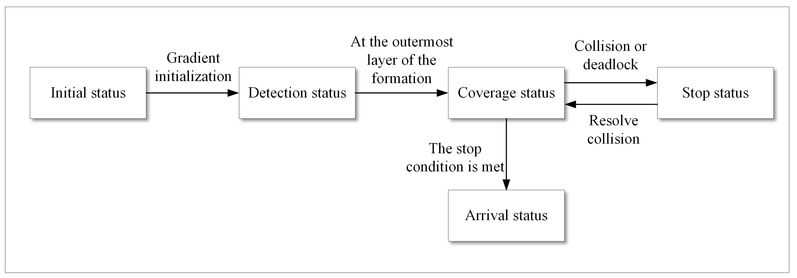
However, different from the single group coverage, the simultaneous coverage of multiple groups of robots will lead to collisions and deadlock problems among different groups of robots. To solve these two problems, a Stop status is added in Figure 4 to prevent the robot from the collision and release the deadlock.

As shown in Figure 6, when a collision or deadlock occurs in the Coverage status, the robot will switch to the Stop status and stop its movement temporarily. The robots will not continue to cover the area until there are no more conflicts and deadlocks are lifted.

4.1. Grouping Method

The robots in the swarm robotic system are randomly distributed on the two-dimensional plane and they are divided into several different groups by grouping method. Then each group can perform the covering action in parallel during the covering process, to improve the coverage speed. Some problems need to be considered in the grouping process. (1) The leader robot in the right position should be selected quickly. (2) The number of robots in each group should be about the same. (3) The distance between the groups is large enough to reduce collisions between the robots.

For the initial random distribution of swarm robots, we should first determine the number of groups K, and then K robots will be selected as the current leaders. Each leader robot has a different group number. The leader of the robot broadcasts its group number and location information to other robots. All robots are not isolated, and the communication range of robots is defined as $R_c$ means that all robots in the communication range of robot $\alpha$ are their neighbors.

The swarm robot system will randomly select K robots as the leader robots firstly, and set as $L={\left\{l_k\right\}}_{k=1,2,\dots ,K}$, but the distribution of the initial selected leader robots is not necessarily reasonable. For example, the distance may be close, which will affect the effect of grouping. Therefore, it is necessary to update the leader robots automatically. The leader robot chooses a neighbor as the new leader according to the neighbor’s position and the current position of other leaders. The sum of the distance to other leaders of the new leader robot $l_k^{\prime }$ should be greater than the old leader robot $l_k$, which satisfies the following equation.

$$l_k^{\prime }=\left\{\alpha \mid \alpha \in l_k·N\wedge \alpha \notin L\wedge {\sum }_{l_j\in L\wedge j\ne k}∥\alpha .\mathbf{x}-l_j·\mathbf{x}∥>{\sum }_{l_j\in L\wedge j\ne k}∥l_k·\mathbf{x}-l_j·\mathbf{x}∥\right\}$$

(2)

where $\alpha .N$ represents all neighbor robots within the communication range of robot $\alpha$, and $\alpha .\mathbf{x}$ represents the position of robot $\alpha$ in two-dimensional space. Once a new leader robot satisfies Equation (2), the original leader robot will be replaced. The new leader will find the next robot which satisfies Equation (2) as the next leader robot, so as to complete the update of the leader robot of the whole swarm robot system.

To update the leader robot quickly, we define one farthest hop number $\mathit{h}$ according to the lifetime of the network packet. The message specifying the next new leader should contain $\mathit{h}$, and $\mathit{h}$ will decrease after finding the new leader. The leader whose $\mathit{h}$ value is 0 is the final leader. If there is no new leader in $l_k$’s neighborhood, $\mathit{h}$ should be reduced automatically within a certain period of time. The self-organizing updating algorithm of the leader robot is shown in Algorithm 3.

Algorithm 3 Leader robot self-organizing update algorithm.

Input: the swarm robots A, leader robot number K Output: the new leader robot 1. $\alpha .\mathit{leder}$ = false, $\alpha .\mathit{g}=0;$     //Initialize all robots 2. $\alpha .\mathit{leder}$ = true, $\alpha .\mathit{g}=\{1,2,\dots ,\mathit{k}\}$     $//\mathit{Randomlyselectkrobotsastheleaderrobots}$ 3. if $\alpha .\mathit{leder}$ == true then     //Set the number of hops for all robots 4.     $\alpha .\mathit{h}=h_{\mathit{max}}$; 5. else $\alpha .\mathit{h}=0$; 6. whlie $(\alpha .\mathit{h}!=0)$ 7.     Broadcast robot position $\alpha .\mathbf{x}$ and hop number h; 8.     Calculate the sum of the distances ∑d between $\alpha$ and all its neighbors and other leader      robots; 9.     ${\alpha }^{\prime }.h=\alpha .h-1$; 10.     $\alpha .\mathrm{leder}=\mathrm{false};$ 11.     ${\alpha }^{\prime }.\mathrm{leder}=\mathrm{true};$ 12.     if $\alpha .\mathrm{leder}==\mathrm{false}\mathrm{then}$ 13.         $\alpha .\mathit{h}=0;$ 14.     end if 15. end while

The self-organizing grouping algorithm borrows the idea of the breadth-first search. Each robot that is not in the group will search the neighboring robots in its communication range, and ask whether to join the group according to the distance until a neighbor who has already joined the group is found and joined the group. The adjacent robots of each leader robot will join the group first. Therefore, through this parallel algorithm, K robot groups with K leading robots as the center can be formed. The self-organizing grouping algorithm is shown in Algorithm 4.

Algorithm 4 Self-organizing grouping algorithm.

Input: the swarm robots and K leader robots Output: the swarm robots and K leader robots 1. while $∥\alpha .\mathbf{x}-{\alpha }^{\prime }.\mathbf{x}∥\le R_{\mathrm{c}}\wedge \alpha .h==0$ do 2.     ${\alpha }_{\mathrm{neighbor}}\leftarrow arg\underset{{\alpha }^{\prime }}{min}∥\alpha .\mathbf{x}-{\alpha }^{\prime }.\mathbf{x}∥$; 3.     if ${\alpha }_{\mathrm{neighbor}}·g!=0$ then 4.         $\alpha .g={\alpha }_{\mathrm{neighbor}}.g$; 5.     end if 6. end while

4.2. Aggregation Behavior

Aggregation behavior is to make the groups that have been divided together first to form a relatively regular pattern so that they can better move together in the way of the group to cover the area. During the aggregation process, the robot will have some status transformation, mainly including the following five status. (1) Approach status; (2) Stop status; (3) Pend status; (4) Join status; (5) Arrive status. The transition relationship of these five states is shown in Figure 7.

• Approach status: It is the initial status of the normal robot. and the robot should gradually approach the leader robot.
• Stop status: This is to prevent the robot from colliding with the approaching the leader robot.
• Pend status:The Pend status also stops the robot’s motion because there are robots with Pend status or Arrive status.
• Join status:The robot will approach the group and find a suitable position to join the formation.
• Arrive status:when the robot has found a suitable position, it will stop moving.

The leader robot is in the Arrival status, and the ordinary robot is in the Approach status, which is constantly approaching the leader.

In the Approach status, if the robot detects that there are other Pend, Join or Arrive status within a certain distance $d_{safe}$, it will switch to the Pend status. The Pend status and the Stop status perform similar operations. In addition, if the robot in the Pend status receives the join instruction from the robot in the Arrive status and detects that it will not collide with the robot in the Join status, it will switch to the Join status.The robot should approach the formation until the distance between the robot and a certain Arrive status is $d_{min}$. Then the robot keeps a distance of $d_{min}$ from the formation and moves around until it reaches a suitable position, and then it switches to the Arrive status.

On the one hand, the robot should detect whether there is still space in the $d_{min}$ range around it for the other robot to arrive; on the other hand, the robot should detect the undetermined status robot in the $d_{safe}$ range and sends the status switch instruction. The total flow of aggregation behavior is shown in Figure 8.

4.3. Collision Avoidance

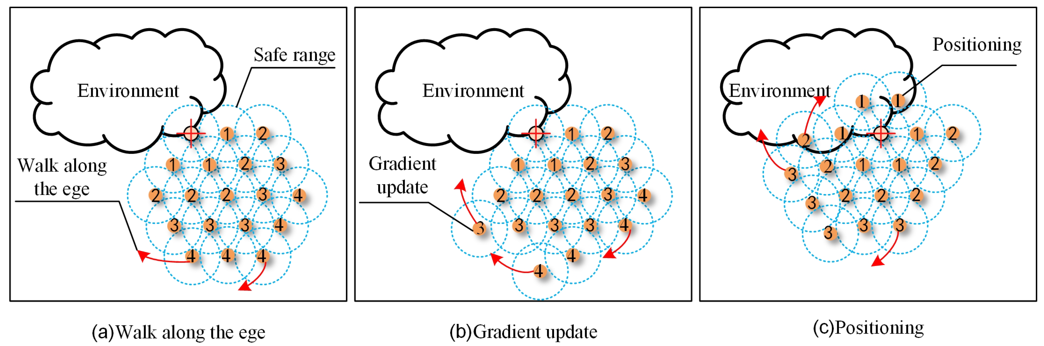
When there is only one group to cover the area, the Detection status of the robot will be converted to the Coverage status in order according to the initial gradient value and ID number, so there is no collision between robots. However, when the number of groups is greater than 2($\mathit{k}\ge 2$), the motion between the robot belonging to different groups cannot be predicted, so it will lead to a collision. As shown in Figure 9, the blue robots are in Arrive status and the yellow robots are in Coverage status. In Figure 9a, the robot ${\alpha }_2$ moves around the robot ${\alpha }_0$, and the robot ${\alpha }_3$ moves around the robot ${\alpha }_1$, which may cause a collision. In Figure 9b, the robot ${\alpha }_4$ moves outside, and the robot ${\alpha }_5$ moves inward, which can also cause a collision.

Once the robot in the Coverage status detects that there are other robots in the Coverage status that are too close to it within the range of $d_{cover}$, the robot will switch to the Stop status. When there are no other robots in the Coverage status within the scope of the robot $d_{cover}$ and no other robots move around it, the Coverage status will be restored.

4.4. Deadlock Detection and Release

In addition to collision avoidance, the grouping method can also cause deadlock. As shown in Figure 9b, if the robot ${\alpha }_5$ detects that the robot ${\alpha }_4$ with the Coverage status in its $d_{cover}$ range, then the robot ${\alpha }_5$ will stop moving until the robot ${\alpha }_4$ has left. The robot ${\alpha }_4$ cannot leave because the robot ${\alpha }_5$ is in the way, then the robot ${\alpha }_4$ is hovering in the same position. While ${\alpha }_4$ and ${\alpha }_5$ are waiting for the other to move first, which leads to the deadlock. Therefore, it is necessary to detect and release the deadlock in time.

$\left(\mathbf{1}\right)\mathbf{Deadlock}\mathbf{detection}$

The position information of the robot is recorded once every time after time $T_r$, and the position information of the two adjacent times is constantly compared. If the Euclidean distance between the two robots is less than the distance threshold $\theta$, it is considered that there is a deadlock that is shown in Equation (3):

$$∥\alpha ·\mathbf{x}\left(\mathrm{t}\right)-\alpha ·\mathbf{x}\left(\mathrm{t}+T_r\right)∥\le \theta$$

(3)

where $\alpha .\mathbf{x}\left(t\right)$ is the current position of robot $\alpha$, $\alpha .\mathbf{x}(t+T_r)$ represents the position of the robot after the time $T_r$, and $\theta$ is the distance threshold. Since the two robots in deadlock must be moving within the $d_{cover}$ range, the maximum value of $\theta$ should not exceed $2\ast d_{cover}$. The deadlock detection algorithm is shown in Algorithm 5.

Algorithm 5 Deadlock detection algorithm.

Input: the robot $\alpha$ in Coverage status Output: update the status of the robot $\alpha$ 1. if $\exists {\alpha }^{\prime }\in A\wedge ∥\alpha .\mathbf{x}-{\alpha }^{\prime }.\mathbf{x}∥\le d_{\mathrm{cover}}\wedge \alpha .\mathrm{status}=\mathrm{Coverage}$ then 2.     $\alpha .status$ = Stop; 3. end if 4. if $∥\alpha .\mathbf{x}\left(\mathrm{t}\right)-\alpha .\mathbf{x}\left(\mathrm{t}+T_r\right)∥\le \theta$ then 5.     if $\exists {\alpha }^{\prime }\in A\wedge {\alpha }^{\prime }.\mathrm{status}!=Stop\wedge \alpha .\mathbf{x}\in D$ then 6.         $\alpha .\mathit{status}$ = Arrive; 7.     else 8.         $\alpha .\mathit{status}$ = Stop; 9.     end if 10. end if

$\left(\mathbf{2}\right)\mathbf{Deadlock}\mathbf{release}$

A robot that detects a deadlock will switch to a Stop status. Unlike a robot that detects a collision and switches to a Stop status, the robot that detects a deadlock may meet the above-mentioned conditions for restoring the cover state, so it should wait for a while before switching to the cover state. The robot that detects the deadlock may meet the conditions for restoring the Coverage status, so it should wait for some time before switching to the Covered status. The deadlock release algorithm is shown in Algorithm 6.

Algorithm 6 Deadlock release algorithm.

Input: the robot $\alpha$ in Stop status Output: update the status of the robot $\alpha$ 1. while ${\mathit{T}}_s\ne 0$ do 2.     if $\forall {\alpha }^{\prime }\in A\wedge ∥\alpha .\mathbf{x}-{\alpha }^{\prime }.\mathbf{x}∥>d_{\mathrm{cover}}$ then 3.         if $!\exists {\alpha }^{\prime \prime }\in A\wedge {\alpha }^{\prime \prime }.\mathbf{v}\leftarrow {\alpha }^{\prime \prime }.\mathbf{v}-{\left({\alpha }^{\prime \prime }.\mathbf{x}-\alpha .\mathbf{x}\right)}^{\mathbf{0}}$ then 4.             $\alpha .\mathit{status}$ = Deploy; 5.         end if 6.     end if 7.     $T_s\leftarrow T_s-1;$ 8. end while

4.5. Grouping-Based Coverage Algorithm

It is important to note that during the coverage based on grouping, $T_r$ needs to be initialized and $\alpha .\mathbf{x}\left(t\right)$ is recorded when the robot switches from the Detection status to the Coverage status. The coverage algorithm based on grouping is shown in Algorithm 7.

Algorithm 7 Coverage algorithm based on grouping.

Input: the robot $\alpha$ without gradient Output: the robot $\alpha$ covered the target area 1. Initialization: all robots are in Initial status, and gradient is initialized to infinity 2. while ($\alpha .\mathit{status}$ != Arrive) do 3.     if $\alpha .\mathit{status}$ == Initial then 4.         Algorithm I: Gradient generation algorithm; 5.     end if 6.     if $\alpha .\mathit{status}$ == Detection then 7.         ${\mathrm{move}}_{allowed}$ = ture; 8.         if $\exists {\alpha }^{\prime }\in A\wedge ∥\alpha .\mathbf{x}-{\alpha }^{\prime }.\mathbf{x}∥\le d_{\mathrm{cover}}$ then 9.             if $\left({\alpha }^{\prime }.grad>\alpha .grad\right)\vee \left({\alpha }^{\prime }.grad=\alpha .grad\wedge {\alpha }^{\prime }.\mathrm{ID}>\alpha .\mathrm{ID}\right)$ then 10.                 ${\mathrm{move}}_{allowed}$ = false; 11.             end if 12.         end if 13.         if ${\mathrm{move}}_{allowed}$ == ture then 14.             if $\alpha .\mathit{status}$ = Deploy; 15.         end if 16.     end if 17.     if $\alpha .\mathit{status}$ == Deploy then 18.         Algorithm IV: Self-organizing grouping algorithm; 19.         Algorithm V: Deadlock detection algorithm; 20.     end if 21.     if $\alpha .\mathit{status}$ == Stop then 22.         Algorithm VI: Deadlock release algorithm; 23.     end if 24. end while

5. Robust Analysis

In the study of swarm robots covering unknown environments, the large number of robots is a prominent feature. In a large number of swarm robots, the failure of individual robots is inevitable. Therefore, the correctness and robustness of the coverage algorithm should be fully considered when studying the coverage algorithm of swarm robots.

In the process of gradient formation, robot $\alpha$ fails to obtain the gradient of its neighbor within the range of $d_{safe}$ due to $\alpha$ fault. In this case, the gradient of $\alpha$ is infinite. There are two situations in the position of robot $\alpha$, as shown in Figure 10. Figure 10a shows that the failure robot is at the edge of the swarm robot group. Since the gradient of $\alpha$ is infinite at this time, according to the region coverage algorithm in algorithm II, the failure robot is in the coverage state first, still moves around the nearest robot, updates the gradient at all times, and finally covers normally. Figure 10b shows that the failure robot is in the closed-loop surrounded by the swarm robot group. At this time, the failure robot $\alpha$ should take the lead in covering. Because the failure robot is surrounded by other robots, it cannot move, and only when the closed-loop is lifted, the failure robot $\alpha$ can move. In both cases, when there is a robot failure, the whole system cannot be brought to a state of paralysis, and the normal coverage task can be completed in the end.

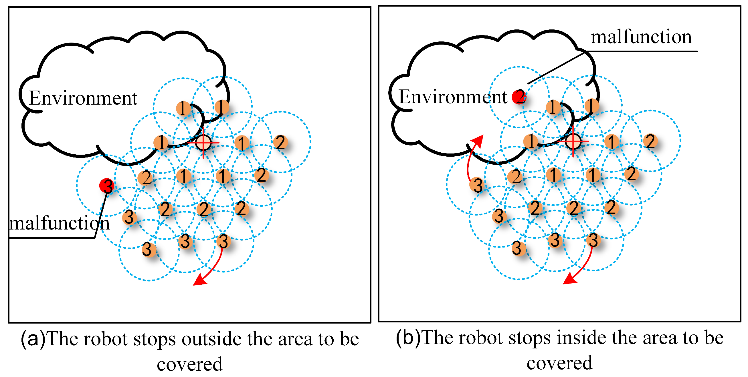
When the swarm robot is covering the region, it stops due to the failure of robot $\alpha$. There are two stopping position states at this time, as shown in Figure 11, which are stopping outside the region to be covered and stopping inside the region to be covered. As shown in Figure 12, when robot $\alpha$ stops outside the area to be covered due to a fault, the status of $\alpha$ at this time is $\alpha .status\ne Coverage$, the gradient of $\alpha$ is $\alpha .grad$, other running robots are also outside the area to be covered, if the around center of the other robot ${\alpha }^{\prime }$ is robot $\alpha$, its gradient will increase adaptively, i.e., ${\alpha }^{\prime }.grad=\alpha .grad+1$, so that ${\alpha }^{\prime }$ can continue the coverage work according to algorithm II. As shown in Figure 13, when robot $\alpha$ stops in the area to be covered due to a fault, at this point, the status of the failure robot $\alpha$ is $\alpha .status=Coverage$, if the other robots in the covering state are centered around robot $\alpha$, they stop moving and line up until ${\alpha }^{\prime \prime }$ reaches the edge of the area to be covered, the status of ${\alpha }^{\prime \prime }$ is ${\alpha }^{\prime \prime }.status\ne Coverage$, if the surround center of other robots is ${\alpha }^{\prime \prime }$, the situation is the same as that of the failure robot $\alpha$ stopping outside the area to be covered.

6. Experiment and Analysis

To evaluate the effectiveness of the proposed method, a series of experiments are carried out to realize the self-organized coverage of the unknown areas by swarm robots. We used multi-agent simulation software Netlogo to experiment. The operating system is Win10, and the hardware resources include 4G memory and I5 CPU processor. The experimental parameters are set as shown in

Table 2. Coverage experiment parameter setting.

$\mathbf{Parameter}\mathbf{Name}$	$\mathbf{Describe}$	$\mathbf{Value}$
${\mathit{d}}_{safe}$	Safe distance	1
${\mathit{d}}_{cover}$	Coverage distance	1, 2, 4, 6, 8, 10
$\mathit{r}$	Coverage radius	4
$\mathbf{v}$	Velocity	0.1
${\mathit{R}}_c$	Communication distance	15

.

To calculate the coverage rate, the target area is divided into a 100 × 100 pixel grid. Coverage rate is represented by the ratio of the number of pixels covered to the total number of pixels in the target area.

6.1. Self-Organizing Coverage Experiment Based on Grouping

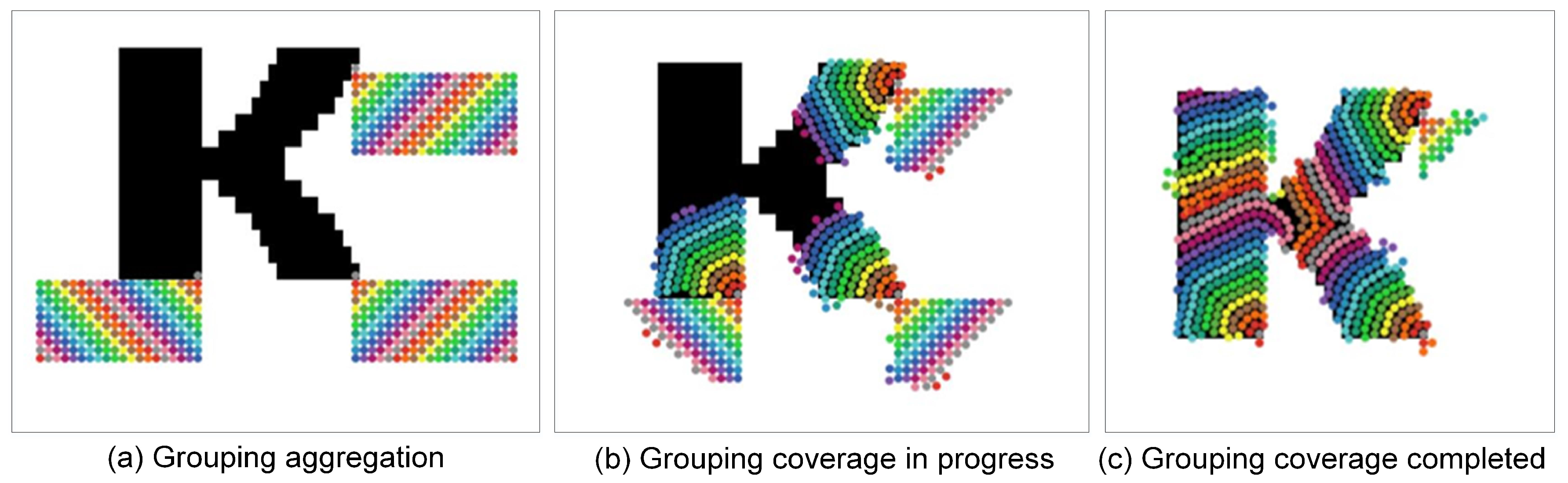
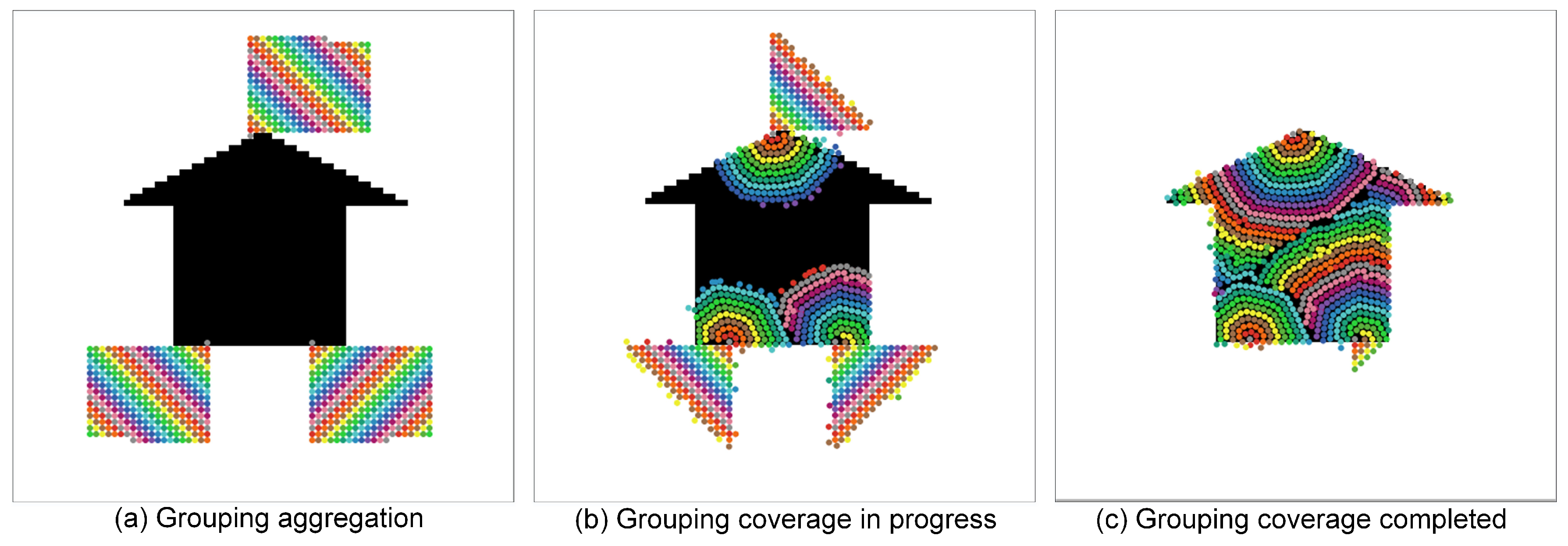
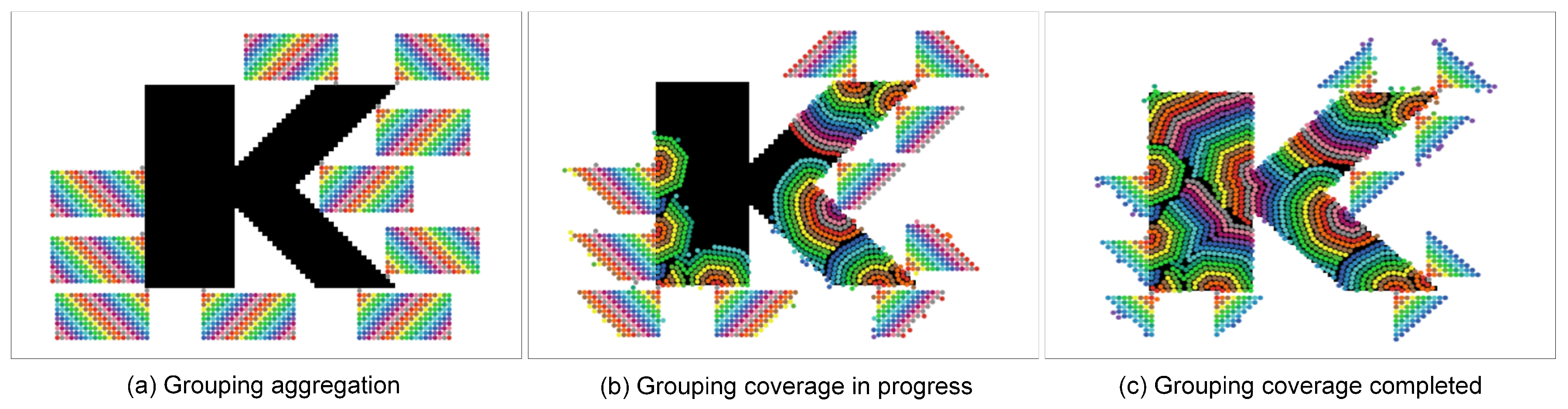
Figure 14 and Figure 15 show the process of self-organizing covering the ’K’ area and the ‘house’ area. There are 603 robots and 942 robots were used respectively, and the number of groups was 3. In Figure 16, a total of 2000 robots are divided into 10 groups to self-organize the ’K’ area.

Different colors of the robot in the figure represent different gradients of the robot (due to the limited number of colors in Netlogo software, 14 different colors are taken as a cycle, i.e., the colors of 0 gradient and 14 gradient are the same, and so on). The gradient-based method can self-organize the coverage of the target area, and the speed of coverage can be improved by the grouping method. Although the experiment demonstrates the effectiveness of the method proposed in this section to cover the target area, some gaps cannot be completely covered at the junction of each group due to the robot conflict between the groups.

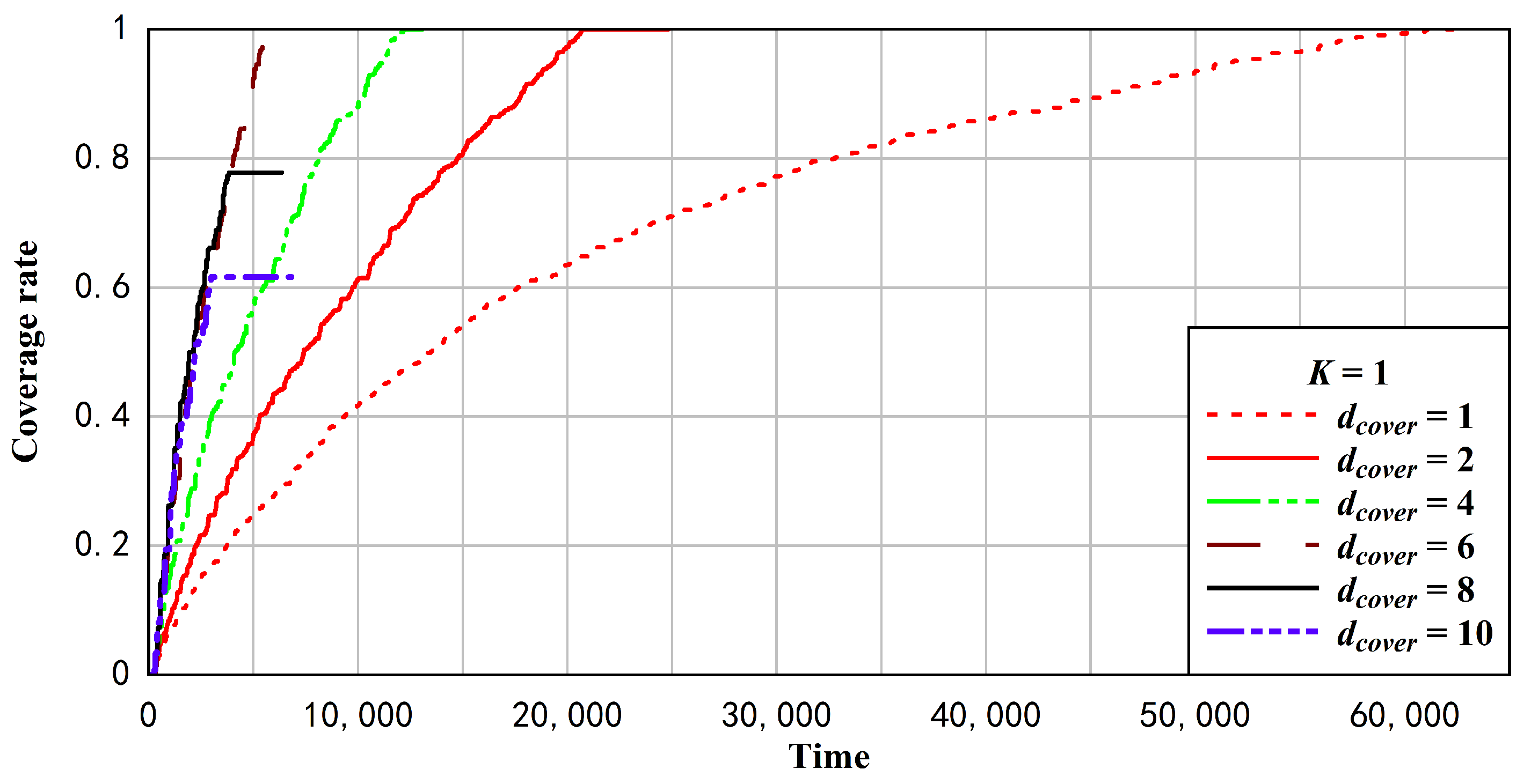
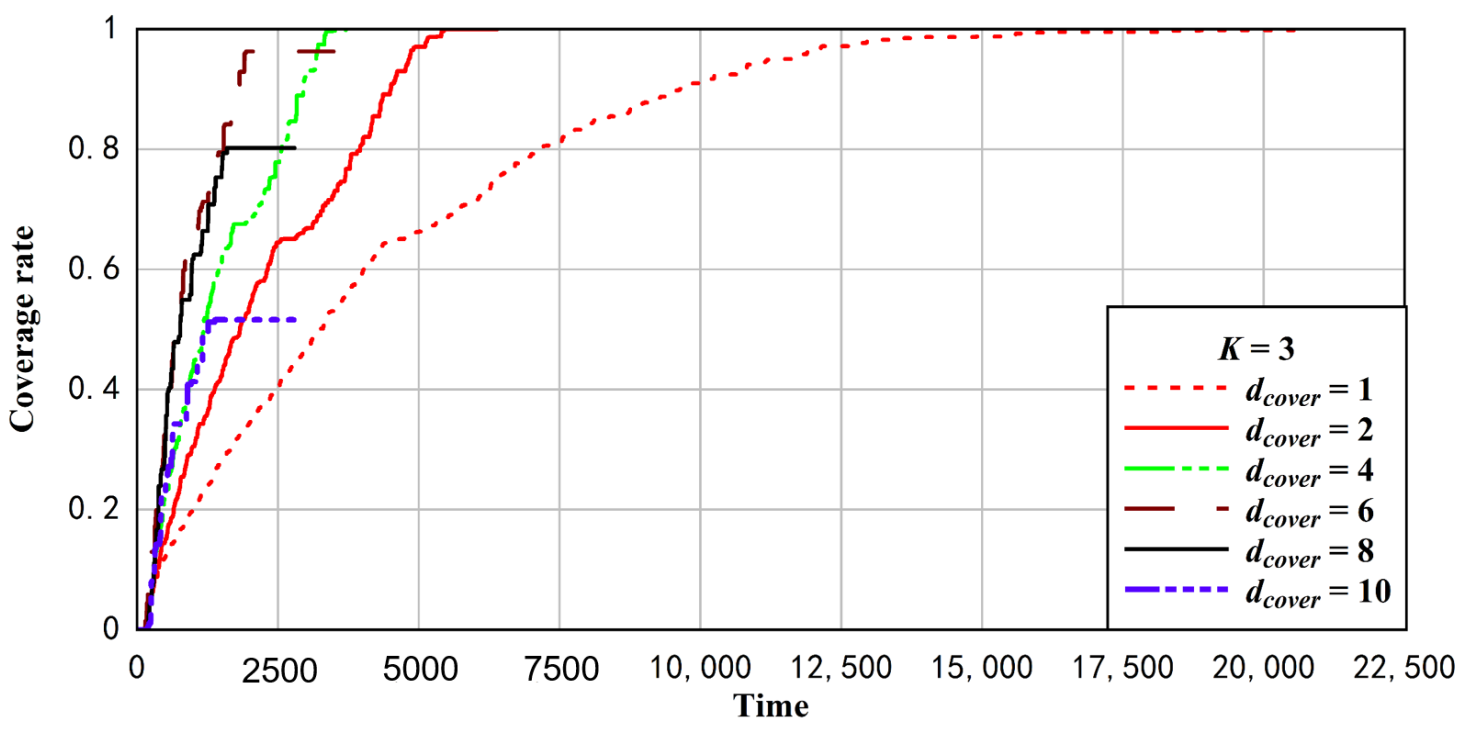
6.2. The Influence of Coverage Radius on Coverage Rate

Keeping other parameter values unchanged, we studied the coverage rate changes with time when the swarm robots were not grouped or the swarm robots were divided into 3 groups, and the coverage distance $d_{cover}$ was 1, 2, 4, 6, 8, and 10 respectively. Repeat the experiment for 30 times for each case and take the average result, as shown in Figure 17 and Figure 18. As can be seen from the figures, the experimental effect is consistent whether the swarm robots are grouping or not. If the number of robots is large enough, as the coverage distance increases, the number of robots for coverage will decrease, and the time for coverage rate to reach a stable level will also decrease, which means that the coverage time will also decrease continuously.

If the coverage radius $\mathit{r}$ of the individual robot remains unchanged, the factors affecting the coverage rate mainly include the coverage distance of the robot and the number of robots entering the coverage area. When the coverage distance of the robot increases to greater than its coverage radius ($d_{cover}>r$), it will lead to the coverage rate less than 100%. The larger the coverage distance is, the smaller the coverage rate will be.

By comparing Figure 17 and Figure 18, we can see some differences between ungrouped coverage and grouping coverage. With the same coverage distance, the stable coverage time of grouping coverage is significantly less than that of without grouping coverage. When the coverage distance is no more than 8, the coverage rate of the two cases is the same. When the coverage distance is equal to 10, it can be seen that in the case of grouping, the coverage rate decreases greatly. The main reason is that when the coverage distance is large, the gaps caused by conflicts between groups will also become larger and larger.

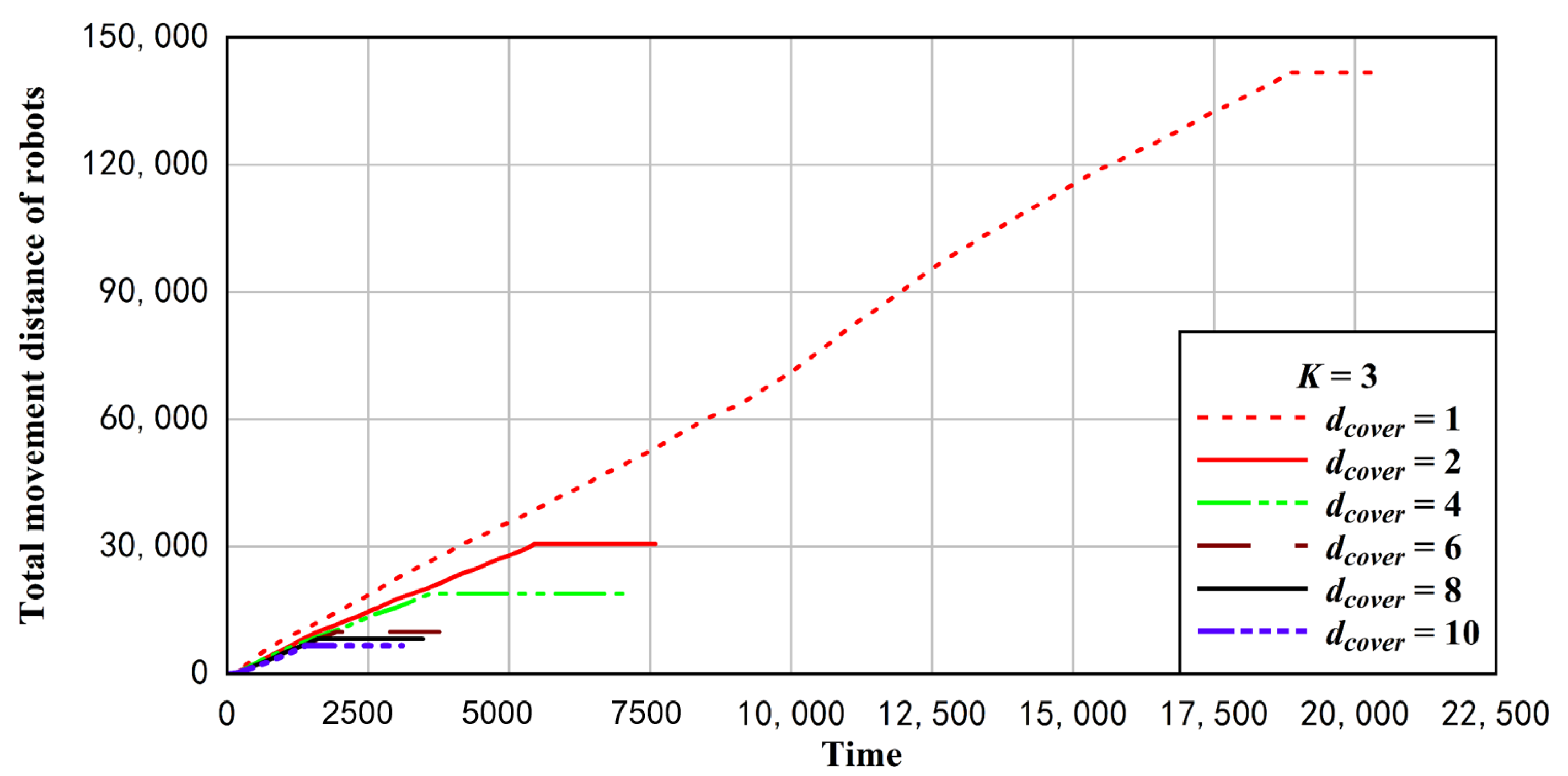
6.3. The Influence of the Number of Groups on the Total Moving Distance of Robots

The total moving distance of the robot reflects the total moving energy consumption of the whole robot system. The smaller the moving distance, the smaller the energy consumption of the robot. It is one of the conditions to judge whether the coverage distance is suitable to discuss the influence of the coverage distance on the total moving distance of the robot. Similarly, keeping other parameters unchanged, we explored the changes of the total moving distance of the robot with time when the covering distance $d_{cover}$ was 1, 2, 4, 6, 8, and 10 when the robot was not grouped or divided into 3 groups. Repeat the experiment for 30 times for each case and take the average result, as shown in Figure 19 and Figure 20.

It can be seen from Figure 19 and Figure 20 that the larger the coverage distance is, the smaller the total moving distance of the swarm robots will be, and the shorter the time for the curve of the total moving distance of the robot to reach a flat level. This is because as the coverage distance increases, the number of robots needed to cover the same area decreases, resulting in a decrease in the total distance traveled by the robots. By comparing Figure 19 and Figure 20, it can be seen that the total moving distance of the swarm robots covered by groups is much smaller than that of the robots not covered by groups. The reason is that in the case of grouping, each group of robots has a smaller size and can enter from different locations in the region at the same time, which makes the maximum radius of the robot surrounding the leader robot with a gradient of 0 smaller, and thus leads to the decrease of the total distance of the robots.

6.4. The Influence of the Number of Groups on the Coverage Rate

As can be seen from the previous experiments, when the robot’s coverage distance $d_{cover}$ is set as 6, various performance measures are relatively good. Therefore, under the condition that $d_{cover}$ is set as 6 and other parameters are the same, we also explored the influence of the number of packets on the coverage. Figure 21 shows the change of average coverage over time in 30 experiments when the number of grouping $\mathit{K}$ is 1, 3, 4, 6, 8, and 10, respectively.

As shown in Figure 21, when the number of groups $\mathit{K}$ is less than 6, the coverage curve of the robot decreases gradually with the increase of the number of groups, and the coverage rate can reach 100%. When the number of groups $\mathit{K}$ varies from 6 to 10, the time when the robot’s coverage curve reaches a plateau increases, and the coverage rate decreases. It can be concluded from the experiment that the increase of the number of robot groups can improve the coverage speed of swarm robotic system to a certain extent, but when the number of groups is too much, the conflicts between different groups will be more and more, which leads to the decrease of coverage rate and the slowing down of coverage speed.

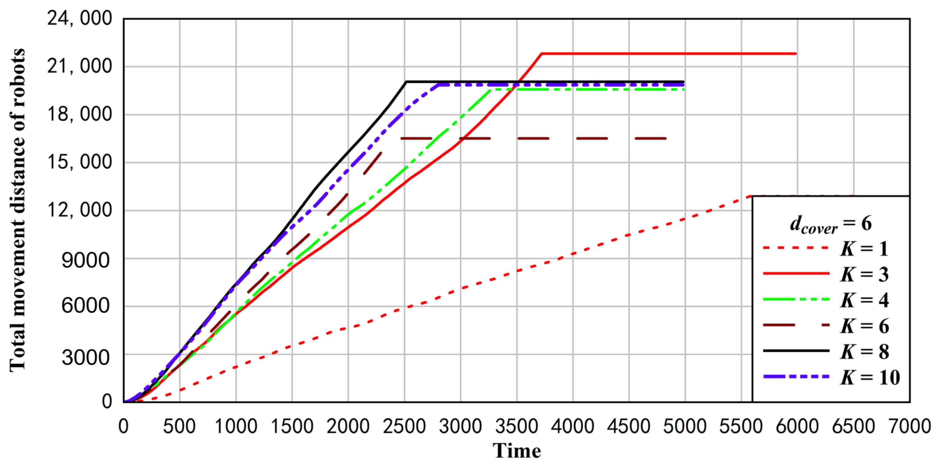
6.5. The Influence of the Number of Groups on the Total Moving Distance of Swarm Robots

When the cover distance is 6 and other parameters are the same, 30 experiments are carried out under the condition of without grouping, 3 groups, 4 groups, 6 groups, 8 groups, and 10 groups, and the total moving distance is analyzed by average value, as shown in Figure 22.

As can be seen from Figure 22, when the swarm robots are not grouped, since there is no inter-group conflict, the distance moved by each robot is the effective distance (that is, it can directly participate in the area coverage without the edge of the area being blocked). The total distance moved by the swarm robotic system is the shortest, but its coverage time is also the longest. When the number of groups is less than 6, the total moving distance of the swarm robots will be shorter with the increase in the number of groups. When the number of robot groups is greater than 6, with the increase of the number of groups, the conflict between groups will increase gradually, which leads to the increase of the total moving distance of the swarm robots.

6.6. Robust Analysis

We studied the coverage completion time and coverage rate of GGC under the condition of no abnormality (failure of individual robots). In large-scale swarm robots, the failure of individual robots is inevitable. Therefore, in the case of a robot failure, it is necessary to analyze the robot’s influence on the experimental results.

The environment was kept consistent, the number of robot groups was set as 3, and the coverage distance was set as 6. In the gradient generation process and the self-organizing coverage process of the robot, 0, 1, 5, 10, and 20 robots were randomly set to fail, which made the robot unable to carry out any work. The experimental results obtained are shown in Figure 23. Figure 23a shows that in the process of gradient formation, a different number of individual robots cannot obtain the gradient of neighbor robots, so the gradient cannot be formed normally. The coverage rate curves shown in the figure roughly coincide. When there are 20 robots with failures, the early coverage speed is faster than the early coverage speed when the other number of robots fail, and this is because the failure robot is close to the leader robot, and the fault robot is at the edge of the swarm robot team. At this point, the gradient of the failure robot is infinite, so that it is in the coverage state first, which reduces the time it takes to move around other robots and faster enters the area to be covered. Figure 23b is the coverage rate and time curve of failures of individual robots in the coverage process. As can be seen from Figure 23b, the curves obtained in all abnormal cases are roughly coincident. When there are 20 robots with failures, the time of other robots moving around the failed robots is increased to some extent, therefore, when N is 20, the coverage speed of the swarm robot is slightly slower in the later stage. In general, the GGC algorithm has good robustness when the robot fails.

6.7. Comparison of Coverage Time and Coverage rate of Different Coverage Algorithms

For the above experiments, the influences of different coverage distances and the number of groups in GGC on the coverage completion time and coverage rate are analyzed, and the optimal coverage distances and number of groups in GGC are obtained. In order to study the advantages of GGC and other coverage algorithms, we conducted experimental analysis and comparison of four coverage algorithms GGC, kilobot [41], DASH [42] and FCDFS [43] in the same coverage environment. We obtained the experimental results, as shown in Figure 24. We intuitively found that the GGC algorithm was optimal in both coverage completion time and coverage. Because the DASH algorithm dynamically adjusts the distance between the robots in real time, the speed of covering completion is relatively slow. In the angle-first (FCDFS) algorithm, the swarm robots continuously enter the area to be covered according to the line state, which makes the curve of the experimental results relatively smooth, at the same time, in the coverage process of the FCDFS algorithm, the arrangement of swarm robots is relatively standard, and there is an interval between adjacent robots, resulting in the coverage rate cannot reach 1. We can also see that the GGC and Kilobot algorithms start to enter the area to be covered after a certain period of time. This is because robots with a higher gradient are the farthest from the area to be covered and need to move around robots with a lower gradient first before they can enter the area to be covered and perform the covering task.

6.8. Qualitative Analysis of Different Coverage Algorithms

In this paper, the GGC algorithm has great advantages in coverage-rate and convergence speed and is also superior to other coverage algorithms in environmental scale, complexity, communication cost, and stability. As shown in

Table 3. Qualitative analysis table of coverage algorithm.

Algorithms	Complex Environment	Communication Delay	Computing Cost	Stability	Coverage Rate	Speed of Convergence
CVT [37]	✗	exist	large	poor	higher	fast
LFS [39]	✗	exist	large	poor	high	slow
DD [40]	✓	exist	large	poor	high	fast
CADT [38]	✗	exist	large	poor	higher	fast
SCWC [33]	✗	not exist	small	good	high	fast
DASH [42]	✓	not exist	small	good	low	slow
FCDFS [43]	✓	not exist	small	poor	high	fast
Kilobot [41]	✓	not exist	small	good	higher	slow
GGC	✓	not exist	small	good	higher	fast

, we can see that other coverage algorithms that do not participate in the quantitative analysis are not suitable for large-scale robot environments and cannot cover complex areas. For CVT, LFS, DD, CADT and other algorithms, there is a large amount of communication between each other and communication delay, and these algorithms require much computation to cover the region. By contrast, GGC does not just adapt to the coverage model of large-scale swarm robots, but also in the same complex area environment, and swarm robots can carry out coverage work with small communication costs and minimal computation. Moreover, because GGC has good robustness, its stability is better than other algorithms.

7. Conclusions and Future Work

In this paper, a method of sensing dynamic gradient only by adjacent robots is proposed, which can effectively realize swarm robots to cover unknown areas by self-organization. Furthermore, the swarm robots are grouped and each group covers the area in parallel to improve the coverage speed. This coverage method can be applied to robots with very simple functions and lack of computing and storage capacity, and the communication cost between robots is very low. Through the experimental analysis, the following conclusions can be drawn: (1) The coverage method based on gradient can make the large-scale robot system self-organize to cover the unknown area effectively; (2) The grouping-based coverage method can effectively improve the regional coverage speed of the swarm robot system and reduce the total moving distance of the swarm robots. However, the number of groups should not be too large, and the coverage distance of the robot should also be taken as a reasonable value. In our future work, other related algorithms will be used to solve the problem of adaptive coverage of dynamically changing regions. Finally, through the application of very simple swarm robots for distributed area coverage, our method can further realize self-organizing control of the collective behavior of submillimeter robots. This will lay the foundation for future microscopic fields such as medicine.