Fernandez–Steel Skew Normal Conditional Autoregressive (FSSN CAR) Model in Stan for Spatial Data

Abstract

In spatial data analysis, the prior conditional autoregressive (CAR) model is used to express the spatial dependence on random effects from adjacent regions. This paper provides a new proposed approach regarding the development of the existing normal CAR model into a more flexible, Fernandez–Steel skew normal (FSSN) CAR model. This approach is able to capture spatial random effects that have both symmetrical and asymmetrical patterns. The FSSN CAR model is built on the basis of the normal CAR with an additional skew parameter. The FSSN distribution is able to provide good estimates for symmetry with heavy- or light-tailed and skewed-right and skewed-left data. The effects of this approach are demonstrated by establishing the FSSN distribution and FSSN CAR model in spatial data using Stan language. On the basis of the plot of the estimation results and histogram of the model error, the FSSN CAR model was shown to behave better than both models without a spatial effect and with the normal CAR model. Moreover, the smallest widely applicable information criterion (WAIC) and leave-one-out (LOO) statistical values also validate the model, as FSSN CAR is shown to be the best model used.

1. Introduction

Spatial analysis is one of the analytic approaches that considers the important aspects of spatial data; that is, data indicated by spatial effects. In general, the figures for spatial data can be estimated using various modeling methods. However, if the spatial effects in the spatial data are not considered, then the estimated model will be imprecise. Data indicating the existence of neighborhood effects, therefore, is very important to analyze spatially and to show that one region affects other regions. For example, it is very important for observed disease or virus data to be considered as spatial data and to be analyzed spatially. This is because diseases or viruses are naturally spread very easily, especially in areas that are close together. Spatial factors are divided into two categories: the geostatistical approach and the lattice approach. In this paper, the lattice approach is used, which means that the spatial influence is set by neighboring regions [1]. The inclusion of spatial lattice effects is added as a random effects component in the model that is not explained in the model without random effects [2]. If spatial effects are not included in the modeling, the results obtained still contain spatial autocorrelation, so that the magnitude of the risk effect between neighboring regions is unknown [2]. On the basis of the research conducted by Rantini et al. [3], the survival model coupled with the normal conditional autoregressive (CAR) spatial effect is considered more representative in modeling correlated spatial data than the survival model without spatial random effects. The spatial dependencies of random effects between regions that are close together are expressed through the prior conditional autoregressive (CAR) model [2,4].

To date, many studies have analyzed spatial data. Research into spatial effects on survival data has been conducted by Banerjee et al. [1]. Their study modeled infant mortality data in Minnesota by employing the Weibull distribution with the normal CAR spatial effect. A similar study was also conducted by Darmofal [2] applying the Weibull distribution on political cases coupled with the normal CAR spatial effect. The Weibull distribution with the normal CAR spatial effect has also been implemented to analyze dengue hemorrhagic fever (DHF) by Iriawan et al. [5]. Another work of DHF data research that also used spatial CAR was presented by Aswi et al. [6]. In their research, the Weibull survival model was given three different prior CAR models: Leroux prior, intrinsic conditionally autoregressive (ICAR) or normal CAR prior, and independent prior models. The other study that used a non-normal CAR model was presented by Motarjem et al. [7]. Their research succeeded in demonstrating a model for asthma data in Tehran by using Weibull distribution coupled with the normal CAR spatial effect, and they compared the result with a non-normal CAR model (the non-normal CAR model used was the double-exponential (DE) CAR model). Model comparison using the normal CAR and DE CAR has also been carried out by Rantini and colleagues [8,9]. Their research demonstrated DHF data modeling in the Pamekasan district, East Java, Indonesia and in the eastern Surabaya, East Java, Indonesia, respectively.

There are several methods for estimating parameters of models. In the Bayesian perspective, one of them is the Hamiltonian Monte Carlo (HMC), which is one of the algorithms of the Markov chain Monte Carlo (MCMC) method, like the Gibbs sampling and Metropolis–Hastings algorithm [10,11,12]. HMC provides a powerful MCMC sampling algorithm [10,13]. There are some advantages in using HMC. Firstly, HMC can converge to the posterior probability density with smaller MCMC samples than required by the derivative-free Metropolis–Hastings algorithm [14]. This is because HMC uses numerical integration schemes by developing the entire system in parallel, consisting of small steps in order to avoid the non-locality problems [11]. Secondly, HMC provides an ergodic Markov chain with high-probability acceptance, even in large transitions [15,16,17]. Thirdly, HMC allows for a more efficient exploration of state space than standard random-walk proposals, due to its high-probability acceptance proposal determination mechanism within the Metropolis–Hastings framework [13]. Fourthly, HMC has better performance compared to the Metropolis or Gibbs samplers, because HMC is able to manage the proposed transitions in the Markov chain that lie far apart in the sampling space [12].

Meanwhile, only spatial modeling with a symmetrical CAR model—i.e., normal CAR and double-exponential (DE) CAR—has been provided in software such as Bayesian inference using Gibbs sampling (BUGS) software [18]. In the BUGS software, “car.normal” and “car.l1” are the functions for the normal CAR and DE CAR model, respectively [18]. An innovation for relaxation of the symmetrical CAR model should be developed by researchers by creating short subprograms as an additional user-defined utility. An open-source programming language, designed as probabilistic programming for Bayesian analysis, is called Stan language, which uses HMC and can be widely used to help in the realization of the relaxation of the symmetrical CAR model. It is rivaling the use of BUGS and the just another Gibbs sampler (JAGS) software that uses MCMC [19]. The efficiency of HMC in achieving inference is faster than the MCMC used in BUGS and JAGS software [19]. In the Stan language, facilities are provided for users to create additional user-defined distributions according to their own programming written in Stan code [20]. This presents a great opportunity for researchers to be more creative in their data-driven analysis. The process of adding a distribution or model as a user-defined in Stan is easier when compared to BUGS and JAGS software. In the research conducted by Wetzels et al. [21], it was found that adding a new distribution to the BUGS program has quite complex steps and requires another program, namely the BlackBox Component Builder. As the BUGS software, adding a new distribution in JAGS is also complicated, which can be seen in research conducted by Wabersich et al. [22]. Stan has its own programming language for defining and adding statistical models [20]. Stan modeling language can be learned through several interfaces in several software. Some of Stan’s interfaces are RStan (R), PyStan (Python), CmdStan (shell, command-line terminal), CmdStanR (R, lightweight wrapper for CmdStan), CmdStanPy (Python, lightweight wrapper for CmdStan), MatlabStan (MATLAB), Stan.jl (Julia), StataStan (Stata), MathematicaStan (Mathematica), ScalaStan (Scala) (see the interfaces in https://mc-stan.org/users/interfaces/). Among these Stan interfaces, R (RStan) and Python (PyStan) are the most popularly used [20]. With Stan’s interface in several software tools, the researcher can generalize the proposed method. In this study, we used RStan.

Considering that there have been many studies using the normal CAR model, Stan provides researchers with a new opportunity to conduct data-driven analysis by incorporating the concept of spatial effect modeling with a non-normal CAR model. Starting with Motarjem et al. [7], using the DE CAR model, researchers could develop another, more flexible non-normal CAR model. In the research by Rantini et al. [8], it was shown that the DE CAR model is no better than the normal CAR model. This research provided evidence that the DE CAR model is not always more robust than the normal CAR, as stated by Motarjem et al. [7]. This is one of the reasons for the proposed Fernandez–Steel skew normal (FSSN) CAR model. Skewness is one of the features of skew-symmetric distributions [23]. Compared to the normal and DE distributions, which can only capture data that have a symmetrical pattern, FSSN distribution is able to be more flexible when explaining both symmetrical and asymmetrical data [24]. In a study conducted by Castillo, et al. [24], who modeled volcanic data with less symmetrical histograms, the FSSN distribution approach would be more favorable than the normal distribution. This fact supports our proposed study, since the distribution of spatial effects is not always symmetrical. One of the advantages of the FSSN distribution over the skew-normal (SN) distribution by Azzalini [25], is that its Fisher information matrix does not have a singularity problem, as occurs with the corresponding Fisher information matrix of the SN distribution [24].

In real-world problems, the size of the data available is not always large enough and it becomes a challenge. This can affect the variation of model parameters [26]. To solve this problem, a fairly strong simulation is suggested, especially through the Bayesian approach [27]. This approach is claimed as a suitable method for data-driven applications [28]. In statistical theory, frequentist approaches are only better for modeling large amounts of data. Bayesian approaches, on the other hand, can be used not only for large data sizes, but also for limited data sizes [26]. To do so, Bayesian emphasizes the accurate choice of priors and simulates for the model. The Monte Carlo simulation becomes effective in dealing with this problem [28,29]. Regarding dependence modeling for small data, Zhang and Shields [30] demonstrated that when the Gaussian dependence assumption is applied, biased estimation results are obtained when the dependence structure deviates from this assumption. The proposed copula dependence was employed to solve their problem. Handling the small data in this study, we proposed to use a simulation with HMC, which is applied to the distribution of non-normal data, namely the FSSN distribution. At the end of this study, it was used on data with spatial dependence.

The aim of this study is to show the new creation of the user-defined FSSN distribution and the FSSN CAR model in Stan and to demonstrate their flexibility to explain the distribution of spatial effects adaptively. The latter exhibits the ability and adaptability to model symmetrical and asymmetrical spatial data patterns. A more mathematical and in-depth explanation of the FSSN distribution can be seen in Fernandez and Steel [31].

This paper is organized as follows. Section 2 introduces the CAR model in general and its mathematical explanation. Section 3 describes the intrinsic conditional autoregressive (ICAR) or normal CAR model. The Stan code for the normal CAR model can be seen in Morris [32]. Further explanation of the normal CAR model derived from the mathematical calculation and applied to the Stan code is given in Appendix A. Section 4 describes the FSSN distribution and the FSSN CAR model and demonstrates the Stan code according to its mathematical description. Section 5 provides several scenarios for simulation studies on univariate and multivariate distributions. Section 6 contains the application and comparison of the normal CAR and FSSN CAR models using the Scotland lip cancer dataset and lung cancer dataset from the London Health Authority. The conclusions are given in Section 7.

2. Conditional Autoregressive (CAR) Model

The area data represents objects defined in terms of geometric features, such as points, lines, polygons, regions, and volumes. The regions are partitioned into a limited number of subregions with clear boundaries. The area data, consisting of a single aggregate size per unit area, could have binary, count, or continuous values. These values can be modeled using the CAR model. The CAR model calculates the proximity between neighboring areas that are close together. According to Besag [33], the area data with a spatial structure show that the neighborhood regions have a higher correlation than those that are far away from each other. Area data are different from point data, which consist of measurements from known geospatial points. While the relationship between regions is given in terms of proximity, the relationship between two regional data points is explained by the unit of distance.

Spatial interactions between a pair of areas $s_i$ and $s_j$ in the given set of observations taken at $n$ different areas of a region can be modeled conditionally as a spatial random variable $\varphi$, which is an $n-$length vector $\mathsf{\varphi }={\left({\varphi }_1,\cdots ,{\varphi }_n\right)}^T$. In CAR models, the spatial relationship between the number of $n$ areas is represented as an adjacency matrix $W$ with dimensions $n\times n$. Each component entry of $w_{i,j}$ and $w_{j,i}$ is positive when the areas $s_i$ and $s_j$ are neighbors, and is zero otherwise. The neighbor’s relationship, written as $s_i\sim s_j$, is defined in terms of this matrix; i.e., the neighbors of the area $s_i$ are those areas that have non-zero entries in a row or column $i$. The conditional distribution for each ${\varphi }_i$ is specified in terms of a mean and precision parameter $\tau$, and can be written as follows [33].

$$p_{\mathrm{Normal}}\left({\varphi }_i|{\varphi }_j,j\ne i,{\tau }_i^{-1}\right)=\mathrm{N}\left(\alpha {\displaystyle \sum _{s_i\sim s_j}{w}_{i,j}}{\varphi }_j,{\tau }_i^{-1}\right),i,j=1,2,\cdots ,n,$$

(1)

where the parameter $\alpha$ controls the strength of the spatial association—when $\alpha =0$, this corresponds to spatial independence—and $n$ is the number of areas in a region.

The corresponding joint distribution can be uniquely determined from the set of full conditional distributions by introducing a fixed point from the support of $p_{\mathrm{Normal}}(.)$. The random vector $\mathsf{\varphi }$ has a multivariate normal standard distribution, and precision parameters are formed from two matrices that describe the neighborhood of $n$ areas; i.e., the diagonal matrix d and the adjacency matrix $W,$ as written in Equation (2) [34].

$$\mathsf{\varphi }\sim {\mathrm{N}}_n\left(0,{\left[D_{\tau }\left(I-\alpha W\right)\right]}^{-1}\right)$$

(2)

where ${\mathrm{N}}_n$ denotes the n-dimensional normal distribution; $\alpha$ is between 0 and 1; d is an $n\times n$ diagonal matrix, where each diagonal entry $d_{i,i}$ contains the number of neighbors of the area $s_i,$ and all off-diagonal entries are zero; $W$ is the adjacency matrix, where entry is $w_{i,j}=1$ if the areas $s_i$ and $s_j$ are neighbors and $w_{i,j}=0$ otherwise, and all diagonal entries $w_{i,i}$ are zero; and I is an $n\times n$ identity matrix.

3. Intrinsic Conditional Autoregressive (ICAR) Model

An intrinsic conditional autoregressive (ICAR) or normal CAR model is a CAR model in which $\alpha$ in Equation (1) is equal to 1. The corresponding conditional distribution specification is expressed as in Equation (3) [32].

$$p_{\mathrm{Normal}}\left({\varphi }_i|{\varphi }_j,j\ne i,{\tau }_i^{-1}\right)=\mathrm{N}\left(\frac{{\displaystyle \sum _{i\sim j}{\varphi }_i}}{d_{i,i}},\frac{1}{d_{i,i}{\tau }_i}\right).$$

(3)

The individual spatial random variable ${\varphi }_i$ for $s_i$ is normally distributed with a mean equal to the average of its neighbors. Its variance decreases as the number of neighbors increases. The joint distribution can be simplified as shown in Equation (4):

$$\mathsf{\varphi }\sim {\mathrm{N}}_n\left(0,{\left[\tau \left(D-W\right)\right]}^{-1}\right),$$

(4)

which rewrites the pairwise difference as shown in Equation (5) (these explanations are given in Appendix A).

$$p_{\mathrm{Normal}}\left(\mathsf{\varphi }|\tau \right)\propto \exp \left\{-\frac{\tau }{2}{\displaystyle \sum _{s_i\sim s_j}{\left({\varphi }_i-{\varphi }_j\right)}^2}\right\}.$$

(5)

A full discussion of ICAR in Stan has been conducted by Morris et al. [32]. In this study, we briefly mention the ICAR or normal CAR model in Stan as an initial introduction.

4. Fernandez–Steel Skew Normal Conditionally Autoregressive (FSSN CAR) Model

Let $\varphi \sim \mathrm{FSSN}\left(\mu ,{\sigma }^2,\delta \right)$ with location, scale, and skewness parameters $-\infty <\mu <\infty$, ${\sigma }^2>0$, and $\delta >0$, respectively. The probability density function (p.d.f) is given in Equation (6).

$$p_{\mathrm{FSSN}}\left(\varphi |\mu ,{\sigma }^2,\delta \right)=\{\begin{array}{ll}\frac{2\delta }{\left[1+{\delta }^2\right]\sigma }g\left(\frac{\delta \left[\varphi -\mu \right]}{\sigma }\right),& \mathrm{if}\varphi <\mu ,\\ \frac{2\delta }{\left[1+{\delta }^2\right]\sigma }g\left(\frac{\left[\varphi -\mu \right]}{\delta \sigma }\right),& \mathrm{if}\varphi \ge \mu ,\end{array}$$

(6)

where $g$ and $G$ denote the standard normal p.d.f and cumulative distribution function (CDF), respectively [24]. Let $\varphi \sim \mathrm{FSSN}\left(\mu ,{\sigma }^2,\delta \right)$, with the mean and variance given by

$\mathrm{E}\left[\varphi \right]=\mu +\frac{\sqrt{2}\sigma \left({\delta }^2-1\right)}{\sqrt{\pi }\delta }$ and $\mathrm{Var}\left(\varphi \right)=\frac{{\sigma }^2\left\{\left(\pi -2\right){\delta }^6+2{\delta }^2\left({\delta }^2+1\right)+\pi -2\right\}}{\pi {\delta }^2\left(1+{\delta }^2\right)}$, respectively [24]. Then, we have relationship between $\mu$ and the mean, as well as ${\sigma }^2$ and variance, as

$\mu =\mathrm{E}\left[\varphi \right]-\frac{\sqrt{2}\sigma \left({\delta }^2-1\right)}{\sqrt{\pi }\delta }$ and ${\sigma }^2=\frac{\pi {\delta }^2\left(1+{\delta }^2\right)\mathrm{Var}\left(\varphi \right)}{\left(\pi -2\right){\delta }^6+2{\delta }^2\left({\delta }^2+1\right)+\pi -2}$, respectively.

Equation (6) can be written as follows:

$$p_{\mathrm{FSSN}}\left(\varphi |\mu ,{\sigma }^2,\delta \right)=\frac{2\delta }{\left[1+{\delta }^2\right]}\frac{1}{\sqrt{2\pi {\sigma }^2}}\exp \left[\left(-\frac{1}{2}{\left(\frac{\left(\varphi -\mu \right)}{\sigma }\right)}^2\right)\left\{{\delta }^2{I}_{\left[\varphi <\mu \right]}\left(\varphi \right)+\frac{1}{{\delta }^2}{I}_{\left[\varphi \ge \mu \right]}\left(\varphi \right)\right\}\right].$$

(7)

The construction of multivariate skewed distributions is based on linear transformations of univariate skewed distributions [35]. Let $n$ be the dimension of the spatial random variable $\mathsf{\varphi }={\left({\varphi }_1,\cdots ,{\varphi }_n\right)}^T\in {\mathcal{R}}^n$, with mean vector $\mathsf{\mu }={\left({\mu }_1,{\mu }_2,\cdots ,{\mu }_n\right)}^T\in {\mathcal{R}}^n$, the $n\times n$ positive definite variance-covariance matrix $\Sigma$, and skewed parameters vector $\mathsf{\delta }={\left({\delta }_1,{\delta }_2,\cdots ,{\delta }_n\right)}^T\in {\mathcal{R}}_{+}^n$; the multivariate FSSN p.d.f can be written as follows [35]:

$$p_{\mathrm{FSSN}}\left(\mathsf{\varphi }|\mu ,\Sigma ,\delta \right)={\displaystyle \prod _{i=1}^n{p}_{FSSN}\left({\varphi }_i|{\mu }_i,{\sigma }_i{}^2,{\delta }_i\right)}$$

(8)

where each $p_{\mathrm{FSSN}}\left({\varphi }_i|{\mu }_i,{\sigma }_i{}^2,{\delta }_i\right)$ is as in Equation (7). The p.d.f of the multivariate FSSN, therefore, can be written as follows:

$$\begin{array}{cc}\hfill p_{\mathrm{FSSN}}\left(\mathsf{\varphi }|\mu ,\sum ,\delta \right)& ={\displaystyle \prod _{i=1}^n{p}_{FSSN}\left({\varphi }_i|{\mu }_i,{\sigma }_i{}^2,{\delta }_i\right)}\hfill \\ \hfill & ={\displaystyle \prod _{i=1}^n\frac{2{\delta }_i}{\left[1+{\delta }_i{}^2\right]}\frac{1}{\sqrt{2\pi {\sigma }_i{}^2}}\exp \left[\left(-\frac{1}{2}{\left(\frac{\left({\varphi }_i-{\mu }_i\right)}{{\sigma }_i}\right)}^2\right)\left\{{\delta }_i{}^2{I}_{\left[{\varphi }_i<{\mu }_i\right]}\left({\varphi }_i\right)+\frac{1}{{\delta }_i{}^2}{I}_{\left[{\varphi }_i\ge {\mu }_i\right]}\left({\varphi }_i\right)\right\}\right]}.\hfill \end{array}$$

(9)

The individual spatial random variable ${\varphi }_i$ for $s_i$ has an FSSN distribution with a mean and variance equal to the normal distribution in Equation (3) and a skew parameter $\delta >0$. The joint distribution can be simplified as in Equation (10):

$$\mathsf{\varphi }\sim {\mathrm{FSSN}}_n\left(0,{\left[\tau \left(D-W\right)\right]}^{-1},\delta \right)$$

(10)

where we set $\tau =1$, so $\mathsf{\varphi }\sim {\mathrm{FSSN}}_n\left(0,{\left[D-W\right]}^{-1},\delta \right)$; thus, we obtain a p.d.f as in Equation (11):

$$\begin{array}{cc}\hfill p_{\mathrm{FSSN}}\left(\mathsf{\varphi }|0,{\left[D-W\right]}^{-1},\delta \right)& ={\displaystyle \prod _{i=1}^n{p}_{FSSN}\left({\varphi }_i{|0,\left(d_{i,i}-w_{i,i}\right)}^{-1},{\delta }_i\right)}\hfill \\ \hfill & ={\displaystyle \prod _{i=1}^n\left(\frac{2{\delta }_i}{1+{\delta }_i{}^2}\right)\frac{1}{\sqrt{2\pi {\left(d_{i,i}-w_{i,i}\right)}^{-1}}}{Q}_i}\hfill \end{array}$$

(11)

where ${\mathrm{Q}}_i=\exp \left[\left(-\frac{1}{2}\frac{{\varphi }_i{}^2}{{\left(d_{i,i}-w_{i,i}\right)}^{-1}}\right)\left\{{\delta }_i{}^2{I}_{\left[{\varphi }_i<0\right]}\left({\varphi }_i\right)+\frac{1}{{\delta }_i{}^2}{I}_{\left[{\varphi }_i\ge 0\right]}\left({\varphi }_i\right)\right\}\right].$ Since $\frac{1}{\sqrt{2\pi {\left(d_{i,i}-w_{i,i}\right)}^{-1}}}$ is a constant, Equation (11) can be rewritten in a proportional form as follows:

$$p_{\mathrm{FSSN}}\left(\mathsf{\varphi }|0,{\left[D-W\right]}^{-1},\delta \right)\propto {\displaystyle \prod _{i=1}^n\left(\frac{2{\delta }_i}{1+{\delta }_i{}^2}\right)\exp \left[\left(-\frac{1}{2}\frac{{\varphi }_i{}^2}{{\left(d_{i,i}-w_{i,i}\right)}^{-1}}\right)\left\{{\delta }_i{}^2{I}_{\left[{\varphi }_i<0\right]}\left({\varphi }_i\right)+\frac{1}{{\delta }_i{}^2}{I}_{\left[{\varphi }_i\ge 0\right]}\left({\varphi }_i\right)\right\}\right]},$$

(12)

with explanations analogous to Appendix A. In logarithmic form, the pairwise difference formulation can be expressed as in Equation (13):

$$\begin{array}{cc}\hfill \log \left(p_{\mathrm{FSSN}}\left(\mathsf{\varphi }|0,{\left[D-W\right]}^{-1},\delta \right)\right)& ={\displaystyle \sum _{i=1}^n\left(\log 2+\log {\delta }_i-\log \left(1+{\delta }_i{}^2\right)-\frac{1}{2}\left(\frac{{\varphi }_i{}^2}{{\left(d_{i,i}-w_{i,i}\right)}^{-1}}\right)\left\{{\delta }_i{}^2{I}_{\left[{\varphi }_i<0\right]}\left({\varphi }_i\right)+\frac{1}{{\delta }_i{}^2}{I}_{\left[{\varphi }_i\ge 0\right]}\left({\varphi }_i\right)\right\}\right)}\hfill \\ \hfill & ={\displaystyle \sum _{i=1}^n\left(\log 2+\log {\delta }_i-\log \left(1+{\delta }_i{}^2\right)-\frac{1}{2}{\left({\varphi }_i-{\varphi }_j\right)}^2\left\{{\delta }_i{}^2{I}_{\left[{\varphi }_i<0\right]}\left({\varphi }_i\right)+\frac{1}{{\delta }_i{}^2}{I}_{\left[{\varphi }_i\ge 0\right]}\left({\varphi }_i\right)\right\}\right)}\hfill \end{array}$$

(13)

where, for $s_i\sim s_j$, it means that $s_i$ neighbors $s_j$ and $i\ne j.$

4.1. Adding FSSN Distribution in Stan

As stated in the Introduction, based on Wetzels et al. [21], adding a new distribution to the BUGS software is extremely complicated and requires another specialized program, namely the BlackBox Component Builder. Likewise in the JAGS software, adding a new distribution also has difficult steps, as stated by Wabersich et al. [22]. Unlike the BUGS and JAGS programs, Stan makes it easy for its users to add new distributions. By knowing the mathematical form of the distribution to be added, the steps added in Stan can be written according to the mathematical calculation steps of the distribution. This convenience provides an advantage for researchers to add new distributions, such as the CAR model. The addition of custom distribution in Stan has already been explained by Annis et al. [20]. Therefore, Stan was chosen as an implementation method for spatial modeling involving adaptive distribution for FSSN. Based on Equation (7), the addition of the user-defined FSSN distribution Stan code can be seen in Listing 1.

Listing 1. A user-defined Stan code of Fernandez–Steel skew normal (FSSN) distribution.

functions{    real FSSN_lpdf(real x, real mu, real sigma, real delta){      real logpdf;      real z;      real delta2;      delta2=delta*delta;      if(sigma<=0)        reject("sigma <= 0; found sigma =", sigma);      if(delta<=0)        reject("delta<=0; found delta =", delta);      z=(x−mu);      if(x<mu){        logpdf=normal_lpdf(delta*z|0,sigma)+log(2)+log(delta)-log1p(delta2);      }      else{        logpdf=normal_lpdf(z/delta|0,sigma)+log(2)+log(delta)-log1p(delta2);      }      return logpdf;    }  }

4.2. Adding the FSSN CAR Model in Stan

Additions to the normal CAR or ICAR model in Stan can be seen in Morris et al. [32]. In this study, the proposed user-defined Stan code for the FSSN CAR model was created. Based on Equation (13), the Stan code for the FSSN CAR model can be seen in Listing 2.

Listing 2. A user-defined Stan code for the FSSN conditional autoregressive (CAR) model.

real car_FSSN_lpdf(vector phi, int N, int[] node1, int[] node2, vector delta){   vector [N] logpdf;   vector [N] delta2   vector [N] phi2;   for(i in 1:N){   delta2[i]=delta[i]*delta[i];   phi2[i]=(phi[node1][i]- phi[node2][i])*(phi[node1][i]- phi[node2][i]);   if(delta[i]<=0)   reject("delta[i]<=0; found delta[i] =", delta[i])   }   for(i in 1:N){   if(phi[i]<0)   logpdf[i]=log(2)+log(delta[i])-log1p(delta2[i])-0.5*delta2[i]*phi2[i]   +FSSN_lpdf(sum(phi)|0,0.001*N,mean(delta));   else   logpdf[i]=log(2)+log(delta[i])-log1p(delta2[i])-0.5*(1/delta2[i])*phi2[i]   +FSSN_lpdf(sum(phi)|0,0.001*N,mean(delta));   }   return sum(logpdf);   }

5. Simulation Study

5.1. Simulation for Univariate Distribution

From Equation (7), it can be seen that, when the value of the skewness parameter $\delta =1$, the FSSN distribution exhibits a normal distribution, with the parameters $\mu$ and ${\sigma }^2$ being the same with those of the FSSN distribution. Thus, to be able to validate the user-defined FSSN distribution in the Stan program, data are generated from a normal distribution ($\mu$, ${\sigma }^2$), giving Stan the opportunity to perform an estimation using the user-defined FSSN. The proof of the validity of FSSN in terms of detecting normal data is that it must be able to estimate $\mu$ and ${\sigma }^2$ correctly in accordance with the generator parameters. Another important factor is the user-defined FSSN must also provide an estimate of $\delta =1$, which means the FSSN must also state that the estimated data exhibit symmetry.

Next, we provide evidence of the application of the FSSN CAR model in Stan. Here, we created 24 scenarios that involved normal, DE, and Student-t distributions. These three distributions are already built-in utilities in Stan, and were proposed to be estimated using FSSN distribution as the user-defined Stan code. These scenarios contain a difficult scheme, which was used to test the ability of the FSSN to detect data with very different variances and zero-centered data with extreme leptokurtic properties. Each scenario was designed using sample sizes of 125, 250, 500, and 1000, generated from normal, DE, and Student-t distributions. Each scenario was replicated 500 times.

The parameter estimation was done by utilizing the HMC facility in Stan through 4 chains and 10,000 iterations. The 24 scenarios for the normal, DE, and Student-t distributions are displayed in

Table 1. Twenty-four scenario simulations for univariate normal (N), double-exponential (DE), and Student-t (T) distributions.

Distribution	Scenario	Sample Size
Normal (0,2)	N1-125	125
	N1-250	250
	N1-500	500
	N1-1000	1000
Normal (0,10)	N2-125	125
	N2-250	250
	N2-500	500
	N2-1000	1000
DE (0,1)	DE1-125	125
	DE1-250	250
	DE1-500	500
	DE1-1000	1000
DE (0,4)	DE2-125	125
	DE2-250	250
	DE2-500	500
	DE2-1000	1000
t (5)	T1-125	125
	T1-250	250
	T1-500	500
	T1-1000	1000
t (7)	T2-125	125
	T2-250	250
	T2-500	500
	T2-1000	1000

.

From the 24 scenarios above, we obtained the highest posterior density (HPD) interval for each parameter as seen in

Table 2. The 95% highest posterior density (HPD) interval for the estimated parameters of 24 scenario simulations for normal (N), double-exponential (DE), and Student-t (T) distributions.

Scenario	Distribution	Targeted Parameter			95% HPD Interval of Estimated Parameter
		$\mathit{\mu }$	$\mathit{\sigma }$	$\mathit{\delta }$	$\widehat{\mathit{\mu }}$		$\widehat{\mathit{\sigma }}$		$\widehat{\mathit{\delta }}$
					LL	UL	LL	UL	LL	UL
N1-125	Normal	0	2	-	−0.0765	0.0866	1.9100	2.0847	-	-
	FSSN	0	2	1	−0.0435	0.0404	1.9095	2.0842	0.9295	1.0776
N1-250	Normal	0	2	-	−0.0878	0.0910	1.8988	2.1010	-	-
	FSSN	0	2	1	−0.0580	0.0505	1.8975	2.0991	0.9420	1.0640
N1-500	Normal	0	2	-	−0.0971	0.1005	1.9071	2.0822	-	-
	FSSN	0	2	1	−0.0598	0.0701	1.9065	2.0815	0.9522	1.0504
N1-1000	Normal	0	2	-	−0.0875	0.0843	1.9260	2.0713	-	-
	FSSN	0	2	1	−0.0793	0.0722	1.9253	2.0703	0.9627	1.0417
N2-125	Normal	0	10	-	−0.0241	0.0228	9.9718	10.0355	-	-
	FSSN	0	10	1	−0.0092	0.0093	9.9722	10.0355	0.9182	1.0829
N2-250	Normal	0	10	-	−0.0302	0.0275	9.9643	10.0450	-	-
	FSSN	0	10	1	−0.0126	0.0130	9.9628	10.0435	0.9412	1.0593
N2-500	Normal	0	10	-	−0.0411	0.0437	9.9418	10.0645	-	-
	FSSN	0	10	1	−0.0177	0.0174	9.9423	10.0635	0.9537	1.0483
N2-1000	Normal	0	10	-	−0.0593	0.0552	9.9303	10.0701	-	-
	FSSN	0	10	1	−0.0247	0.0250	9.9302	10.0701	0.9656	1.0345
DE1-125	DE	0	1	-	−0.0912	0.0966	0.9005	1.0875	-	-
	FSSN	0	1	1	−0.0740	0.0648	0.8572	1.1086	0.8844	1.1172
DE1-250	DE	0	1	-	−0.0704	0.0761	0.9183	1.0870	-	-
	FSSN	0	1	1	−0.0776	0.0755	0.8864	1.1027	0.9058	1.1196
DE1-500	DE	0	1	-	−0.0522	0.0620	0.9361	1.0745	-	-
	FSSN	0	1	1	−0.0766	0.0792	0.9166	1.0911	0.9219	1.0877
DE1-1000	DE	0	1	-	−0.0432	0.0399	0.9487	1.0608	-	-
	FSSN	0	1	1	−0.0701	0.0731	0.9306	1.0661	0.9252	1.0750
DE2-125	DE	0	4	-	−0.0691	0.0680	3.9499	4.0466	-	-
	FSSN	0	4	1	−0.0282	0.0254	3.9008	4.0846	0.8866	1.1167
DE2-250	DE	0	4	-	−0.0775	0.0838	3.9363	4.0647	-	-
	FSSN	0	4	1	−0.0363	0.0360	3.8720	4.1196	0.9173	1.1045
DE2-500	DE	0	4	-	−0.0887	0.1013	3.9248	4.0820	-	-
	FSSN	0	4	1	−0.0498	0.0517	3.8554	4.1497	0.9376	1.0717
DE2-1000	DE	0	4	-	−0.1014	0.0927	3.9093	4.0986	-	-
	FSSN	0	4	1	−0.0639	0.0678	3.8340	4.1506	0.9421	1.0520
T1-125	t	-	-	-	-	-	-	-	-	-
	FSSN	0	1.2910	1	−0.0668	0.0736	1.1381	1.4270	0.8834	1.1129
T1-250	t	-	-	-	-	-	-	-	-	-
	FSSN	0	1.2910	1	−0.0853	0.0965	1.1577	1.4448	0.8904	1.1189
T1-500	t	-	-	-	-	-	-	-	-	-
	FSSN	0	1.2910	1	−0.1093	0.1294	1.1773	1.4268	0.9020	1.1053
T1-1000	t	-	-	-	-	-	-	-	-	-
	FSSN	0	1.2910	1	−0.1242	0.1299	1.2021	1.3881	0.9068	1.1023
T2-125	t	-	-	-	-	-	-	-	-	-
	FSSN	0	1.1832	1	−0.0638	0.0648	1.0598	1.3055	0.8954	1.1035
T2-250	t	-	-	-	-	-	-	-	-	-
	FSSN	0	1.1832	1	−0.0848	0.0778	1.0718	1.2841	0.9095	1.0980
T2-500	t	-	-	-	-	-	-	-	-	-
	FSSN	0	1.1832	1	−0.1002	0.1037	1.1027	1.2808	0.9214	1.0938
T2-1000	t	-	-	-	-	-	-	-	-	-
	FSSN	0	1.1832	1	−0.1082	0.0946	1.1086	1.2488	0.9339	1.0763

LL and UL are the lower limit and upper limit of the HPD interval, respectively.

. To complete the parameter estimation results that were carried out on the simulation data with the 500 replications above, the bias, the root-mean-squared error (RMSE), and the coverage probability (CP) are given in

Table 3. Bias for the estimated parameters of 24 scenario simulations for normal (N), double-exponential (DE), and Student-t (T) distributions.

Scenario	Distribution	Targeted Parameter			Bias of the Estimated Parameter
		$\mathit{\mu }$	$\mathit{\sigma }$	$\mathit{\delta }$	$\widehat{\mathit{\mu }}$	$\widehat{\mathit{\sigma }}$	$\widehat{\mathit{\delta }}$
N1-125	Normal	0	2	-	0.00133	0.00112	-
	FSSN	0	2	1	0.00054	−0.00038	0.00295
N1-250	Normal	0	2	-	−0.00331	−0.00049	-
	FSSN	0	2	1	−0.00251	−0.00190	0.00066
N1-500	Normal	0	2	-	0.00273	−0.00152	-
	FSSN	0	2	1	0.00111	−0.00267	0.00180
N1-1000	Normal	0	2	-	0.00105	0.00155	-
	FSSN	0	2	1	−0.00033	0.00064	0.00120
N2-125	Normal	0	10	-	−0.00005	0.00200	-
	FSSN	0	10	1	−0.00030	0.00070	0.00300
N2-250	Normal	0	10	-	−0.00050	0.00080	-
	FSSN	0	10	1	−0.00010	0.00020	0.00020
N2-500	Normal	0	10	-	−0.00200	−0.00030	-
	FSSN	0	10	1	−0.00060	−0.00090	−0.00200
N2-1000	Normal	0	10	-	−0.00200	−0.00100	-
	FSSN	0	10	1	−0.00100	−0.00200	0.00004
DE1-125	DE	0	1	-	0.00201	0.00170	-
	FSSN	0	1	1	0.00172	−0.00721	0.00198
DE1-250	DE	0	1	-	0.00104	0.00130	-
	FSSN	0	1	1	−0.00126	−0.00463	0.00449
DE1-500	DE	0	1	-	0.00227	0.00290	-
	FSSN	0	1	1	0.00061	−0.00195	0.00192
DE1-1000	DE	0	1	-	−0.00110	0.00398	-
	FSSN	0	1	1	−0.00068	0.00045	0.00039
DE2-125	DE	0	4	-	0.00150	−0.00040	-
	FSSN	0	4	1	0.00052	−0.00590	0.00250
DE2-250	DE	0	4	-	0.00130	−0.00120	-
	FSSN	0	4	1	−0.00097	−0.00640	0.00380
DE2-500	DE	0	4	-	0.00370	0.00079	-
	FSSN	0	4	1	0.00008	−0.00450	0.00170
DE2-1000	DE	0	4	-	−0.00250	0.00450	-
	FSSN	0	4	1	−0.00077	0.00018	−0.00028
T1-125	t	-	-	-	-	-	-
	FSSN	0	1.2910	1	−0.00126	−0.00980	0.00309
T1-250	t	-	-	-	-	-	-
	FSSN	0	1.2910	1	−0.00040	−0.00423	0.00225
T1-500	t	-	-	-	-	-	-
	FSSN	0	1.2910	1	0.00026	−0.00760	0.00133
T1-1000	t	-	-	-	-	-	-
	FSSN	0	1.2910	1	−0.00037	−0.00295	0.00049
T2-125	t	-	-	-	-	-	-
	FSSN	0	1.1832	1	0.00242	−0.00742	0.00004
T2-250	t	-	-	-	-	-	-
	FSSN	0	1.1832	1	−0.00038	−0.00332	0.00191
T2-500	t	-	-	-	-	-	-
	FSSN	0	1.1832	1	−0.00303	−0.00058	0.00399
T2-1000	t	-	-	-	-	-	-
	FSSN	0	1.1832	1	−0.00159	−0.00262	0.00258

,

Table 4. Root-mean-squared error (RMSE) for the estimated parameters of 24 scenario simulations for normal (N), double-exponential (DE), and Student-t (T) distributions.

Scenario	Distribution	Targeted Parameter			RMSE of the Estimated Parameter
		$\mathit{\mu }$	$\mathit{\sigma }$	$\mathit{\delta }$	$\widehat{\mathit{\mu }}$	$\widehat{\mathit{\sigma }}$	$\widehat{\mathit{\delta }}$
N1-125	Normal	0	2	-	0.0424	0.0454	-
	FSSN	0	2	1	0.0215	0.0457	0.0385
N1-250	Normal	0	2	-	0.0478	0.0517	-
	FSSN	0	2	1	0.0279	0.0518	0.0313
N1-500	Normal	0	2	-	0.0506	0.0457	-
	FSSN	0	2	1	0.0346	0.0460	0.0249
N1-1000	Normal	0	2	-	0.0437	0.0385	-
	FSSN	0	2	1	0.0398	0.0385	0.0197
N2-125	Normal	0	10	-	0.0119	0.0163	-
	FSSN	0	10	1	0.0050	0.0161	0.0436
N2-250	Normal	0	10	-	0.0155	0.0206	-
	FSSN	0	10	1	0.0064	0.0206	0.0315
N2-500	Normal	0	10	-	0.0216	0.0306	-
	FSSN	0	10	1	0.0087	0.0306	0.0241
N2-1000	Normal	0	10	-	0.0295	0.0355	-
	FSSN	0	10	1	0.0128	0.0355	0.0178
DE1-125	DE	0	1	-	0.0481	0.0470	-
	FSSN	0	1	1	0.0354	0.0649	0.0579
DE1-250	DE	0	1	-	0.0368	0.0432	-
	FSSN	0	1	1	0.0397	0.0560	0.0532
DE1-500	DE	0	1	-	0.0288	0.0376	-
	FSSN	0	1	1	0.0422	0.0454	0.0443
DE1-1000	DE	0	1	-	0.0212	0.0302	-
	FSSN	0	1	1	0.0387	0.0352	0.0377
DE2-125	DE	0	4	-	0.0355	0.0245	-
	FSSN	0	4	1	0.0137	0.0484	0.0561
DE2-250	DE	0	4	-	0.0415	0.0327	-
	FSSN	0	4	1	0.0191	0.0638	0.0466
DE2-500	DE	0	4	-	0.0480	0.0428	-
	FSSN	0	4	1	0.0269	0.0767	0.0345
DE2-1000	DE	0	4	-	0.0492	0.0508	-
	FSSN	0	4	1	0.0357	0.0821	0.0279
T1-125	t	-	-	-	-	-	-
	FSSN	0	1.2910	1	0.0355	0.0769	0.0593
T1-250	t	-	-	-	-	-	-
	FSSN	0	1.2910	1	0.0468	0.0747	0.0572
T1-500	t	-	-	-	-	-	-
	FSSN	0	1.2910	1	0.0585	0.0633	0.0515
T1-1000	t	-	-	-	-	-	-
	FSSN	0	1.2910	1	0.0678	0.0489	0.0492
T2-125	t	-	-	-	-	-	-
	FSSN	0	1.1832	1	0.0325	0.0609	0.0531
T2-250	t	-	-	-	-	-	-
	FSSN	0	1.1832	1	0.0440	0.0575	0.0489
T2-500	t	-	-	-	-	-	-
	FSSN	0	1.1832	1	0.0526	0.0460	0.0426
T2-1000	t	-	-	-	-	-	-
	FSSN	0	1.1832	1	0.0520	0.0359	0.0361

and

Table 5. Coverage probability (CP) for the estimated parameters of 24 scenario simulations for normal (N), double-exponential (DE), and Student-t (T) distributions.

Scenario	Distribution	Targeted Parameter			CP of the Estimated Parameter (%)
		$\mathit{\mu }$	$\mathit{\sigma }$	$\mathit{\delta }$	$\widehat{\mathit{\mu }}$	$\widehat{\mathit{\sigma }}$	$\widehat{\mathit{\delta }}$
N1-125	Normal	0	2	-	100	100	-
	FSSN	0	2	1	100	100	99
N1-250	Normal	0	2	-	100	99	-
	FSSN	0	2	1	100	99	99
N1-500	Normal	0	2	-	99	98	-
	FSSN	0	2	1	100	98	99
N1-1000	Normal	0	2	-	99	97	-
	FSSN	0	2	1	100	97	100
N2-125	Normal	0	10	-	100	100	-
	FSSN	0	10	1	100	100	96
N2-250	Normal	0	10	-	100	100	-
	FSSN	0	10	1	100	100	98
N2-500	Normal	0	10	-	100	100	-
	FSSN	0	10	1	100	100	97
N2-1000	Normal	0	10	-	100	100	-
	FSSN	0	10	1	100	100	97
DE1-125	DE	0	1	-	97	99	-
	FSSN	0	1	1	100	91	93
DE1-250	DE	0	1	-	97	99	-
	FSSN	0	1	1	100	85	91
DE1-500	DE	0	1	-	96	97	-
	FSSN	0	1	1	99	81	91
DE1-1000	DE	0	1	-	96	96	-
	FSSN	0	1	1	99	76	86
DE2-125	DE	0	4	-	100	100	-
	FSSN	0	4	1	100	100	89
DE2-250	DE	0	4	-	100	100	-
	FSSN	0	4	1	100	99	87
DE2-500	DE	0	4	-	100	100	-
	FSSN	0	4	1	100	96	88
DE2-1000	DE	0	4	-	99	100	-
	FSSN	0	4	1	100	89	86
T1-125	t	-	-	-	-	-	-
	FSSN	0	1.2910	1	100	90	92
T1-250	t	-	-	-	-	-	-
	FSSN	0	1.2910	1	100	83	87
T1-500	t	-	-	-	-	-	-
	FSSN	0	1.2910	1	97	76	82
T1-1000	t	-	-	-	-	-	-
	FSSN	0	1.2910	1	92	77	76
T2-125	t	-	-	-	-	-	-
	FSSN	0	1.1832	1	100	93	95
T2-250	t	-	-	-	-	-	-
	FSSN	0	1.1832	1	100	91	93
T2-500	t	-	-	-	-	-	-
	FSSN	0	1.1832	1	99	86	92
T2-1000	t	-	-	-	-	-	-
	FSSN	0	1.1832	1	96	85	90

, respectively. For example, the bias for the estimated parameter $\widehat{\mu }$ is defined by Equation (14) [36]:

$$\mathrm{bias}\left(\widehat{\mu }\right)=E\left[\widehat{\mu }\right]-\mu$$

(14)

where, if the bias gets closer to zero, the parameter estimation is better. The RMSE for the estimated parameter $\widehat{\mu }$ is defined by Equation (15) [36,37]:

$${\mathrm{RMSE}}_{\widehat{\mu }}=\sqrt{\frac{{\displaystyle \sum _i^{n_{rep}}{\left(\mu -{\widehat{\mu }}_i\right)}^2}}{n_{rep}}}$$

(15)

where $n_{rep}$ is the number of replications, and, if the RMSE gets closer to zero, the parameter estimation is better. The bias and RMSE analogue for other parameters. The coverage probability (CP) is the proportion (in percentage) of the time that the interval contains the true value of interest [38]. When the CP gets closer to 100, the parameter estimation is better.

Some characteristics of the distributions, and the relationship between FSSN and the normal, double-exponential (DE), and Student-t distributions, express the discussion about the HPD interval, bias, RMSE, and CP in the 24 scenarios above. Mathematically, the normal distribution is a special case for the FSSN distribution. When the FSSN distribution has $\delta =1$, it becomes a normal distribution [24]. The double-exponential (DE) distribution is not a special case of the FSSN distribution. It has a symmetrical pattern with fat-tails and could be leptokurtic. Given the simulation data generated from the DE distribution, the FSSN distribution is proposed to be able to estimate and identify the data pattern. Then, the Student-t distribution has the same symmetrical pattern as the normal distribution, but it only has one parameter, namely, degrees of freedom $\nu$. The smaller the $\nu$, the fatter the tails. Its mean is zero with variance is equal to $\frac{\nu }{\nu -2}$. With this information, the FSSN is expected to be able to estimate the data generated from the Student-t distribution with $\mu$ equal to zero, $\sigma$ equal to the $\sqrt{\frac{\nu }{\nu -2}}$, and $\delta =1$ [39].

From Table 2, we can infer that the FSSN distribution is able to estimate the simulation data generated from the normal, DE, and Student-t distributions. This is because the HPD interval for all of the estimated parameter $\widehat{\delta }$ is close to 1. The FSSN distribution succeeds in identifying that each random data point comes from a symmetrical distribution. From Table 3, it can be seen that the biases for the estimated parameters of the FSSN distribution are close to zero. It demonstrates that the FSSN goodness of fit to these generated patterns of data is precisely estimated. Considering Table 4, it can be seen that RMSE for the estimated parameters of the FSSN distribution is smaller than the normal distribution. For scenarios of the generated data from the DE and Student-t distributions, it can be seen that the RMSE for the estimated parameters of the FSSN distribution is close to zero. Considering Table 5 for a normal scenario, the CP for the estimated parameters of the FSSN distribution are more than or equal to the CP for the estimated parameters of the normal distribution. For the DE and Student-t (T) scenarios, some CPs for the estimated parameters of the FSSN distribution are smaller than 80%. This does not mean that the FSSN distribution has poor performance, but rather that the FSSN distribution is adaptively capable of detecting data patterns resulting from the DE and Student-t distributions with the FSSN distribution parameters themselves. This supports the difference in the characteristics of the mathematical representation between DE and Student-t on the FSSN distribution. With the explanation that has been given, two conclusions can be drawn: Firstly, that the FSSN distribution is better than the normal distribution in estimating the data generated from the normal distribution. Secondly, the FSSN distribution is able to estimate the data generated from the DE and Student-t distributions.

5.2. Simulation for Multivariate Distribution

In this subsection, we describe how we simulated for the multivariate extension of the FSSN distribution, as written in Equation (9). In this simulation, we had eight scenarios that involved multivariate normal distribution, keeping in mind that mathematically, the normal distribution is a special case of the FSSN distribution. Each scenario was designed using sample sizes of 50, 100, 150, and 200, generated from trivariate normal distribution ${\mathrm{N}}_3(\mathsf{\mu },\Sigma )$, whereas the number of chains, iterations, and replications were the same as the simulation in the univariate subsection. The eight scenarios are displayed in

Table 6. Eight scenario simulations for multivariate normal (MVN) distribution.

Distribution	Scenario	Sample Size
${\mathrm{N}}_3\left({\mu }_1=\left(\begin{array}{c}0\\ 0\\ 0\end{array}\right),{\Sigma }_1=\left(\begin{array}{ccc}1& 1& 1\\ 1& 2& 1\\ 1& 1& 3\end{array}\right)\right)$	MVN1-50	50
	MVN1-100	100
	MVN1-150	150
	MVN1-200	200
${\mathrm{N}}_3\left({\mu }_2=\left(\begin{array}{c}0\\ 0\\ 0\end{array}\right),{\Sigma }_2=\left(\begin{array}{ccc}4& 1& 1\\ 1& 5& 1\\ 1& 1& 6\end{array}\right)\right)$	MVN2-50	50
	MVN2-100	100
	MVN2-150	150
	MVN2-200	200

.

From the eight scenarios above, we obtained the Euclidean distance for $\left(\mathsf{\mu }-\hat{\mathsf{\mu }}\right)$ and the determinant of the Euclidean distance matrix of $\left(\Sigma -\widehat{\Sigma }\right)$. Meanwhile, when using the trivariate FSSN distribution, besides obtaining these two, we also obtained the Euclidean distance for $\left(\mathsf{\delta }-\hat{\mathsf{\delta }}\right)$. The formula for getting the Euclidean distance and Euclidean distance matrix can be seen in research conducted by Dokmanic et al. [40] and Lele [41], respectively. In mathematics, the Euclidean distance between two points is the length of a line segment between the two points [40]. Then, the interpretation of the determinant matrix is closely related to volume [42]. Thus, the smaller the Euclidean distance and the determinant of the Euclidean distance matrix, the better the parameter estimation. In

Table 7. Euclidean distance and determinant of Euclidean distance matrix for the estimated parameters of eight scenario simulations for multivariate normal (MVN) distribution.

Scenario	Multivariate Distribution	Targeted Parameter			$\mathbf{Euclidean}\mathbf{Distance}\mathbf{of}\left(\mathsf{\mu }-\hat{\mathsf{\mu }}\right)$	$\mathbf{Determinant}\mathbf{of}\mathbf{Euclidean}\mathbf{Distance}\mathbf{Matrix}\mathbf{of}\left(\mathsf{\Sigma }-\hat{\mathsf{\Sigma }}\right)$	$\mathbf{Euclidean}\mathbf{Distance}\mathbf{of}\left(\mathsf{\delta }-\widehat{\mathsf{\delta }}\right)$
		$\mathsf{\mu }$	$\mathsf{\Sigma }$	$\mathsf{\delta }$
MVN1-50	Normal	$\left(\begin{array}{c}0\\ 0\\ 0\end{array}\right)$	$\left(\begin{array}{ccc}1& 1& 1\\ 1& 2& 1\\ 1& 1& 3\end{array}\right)$	$\left(\begin{array}{c}1\\ 1\\ 1\end{array}\right)$	0.00566	$4.3863\times {10}^{-38}$	-
	FSSN				0.00247	$-1.2720\times {10}^{-39}$	0.00002
MVN1-100	Normal				0.00019	$7.1217\times {10}^{-42}$	-
	FSSN				0.00196	$-1.5471\times {10}^{-40}$	0.00606
MVN1-150	Normal				0.00301	$-4.5139\times {10}^{-38}$	-
	FSSN				0.00157	$5.2645\times {10}^{-39}$	0.00515
MVN1-200	Normal				0.00538	$-3.1958\times {10}^{-39}$	-
	FSSN				0.00302	$3.1340\times {10}^{-41}$	0.00123
MVN2-50	Normal	$\left(\begin{array}{c}0\\ 0\\ 0\end{array}\right)$	$\left(\begin{array}{ccc}4& 1& 1\\ 1& 5& 1\\ 1& 1& 6\end{array}\right)$	$\left(\begin{array}{c}1\\ 1\\ 1\end{array}\right)$	0.00753	$-1.9865\times {10}^{-38}$	-
	FSSN				0.00350	$1.9462\times {10}^{-37}$	0.00559
MVN2-100	Normal				0.00294	$-6.0291\times {10}^{-37}$	-
	FSSN				0.00315	$3.4961\times {10}^{-37}$	0.00431
MVN2-150	Normal				0.00163	$4.0158\times {10}^{-38}$	-
	FSSN				0.00009	$1.7077\times {10}^{-38}$	0.00502
MVN2-200	Normal				0.00421	$3.0528\times {10}^{-37}$	-
	FSSN				0.00044	$3.4680\times {10}^{-38}$	0.00611

, the Euclidean distance for the difference between the estimated parameter $\hat{\mathsf{\mu }}$ and the parameter $\mu$, the determinant of the Euclidean distance matrix for the difference between the estimated parameter $\widehat{\Sigma }$ and the parameter $\Sigma$, and the Euclidean distance for the difference between the estimated parameter $\widehat{\delta }$ and the parameter $\delta$, are given.

In Table 7, in the “Euclidean Distance of $\left(\mu -\widehat{\mu }\right)$” column, there are two Euclidean distances for the FSSN distribution that are greater than the normal distribution, namely, in the MVN1-100 and MVN1-200 scenarios. In the “Determinant of Euclidean Distance Matrix of $\left(\Sigma -\widehat{\Sigma }\right)$” column, very small values were obtained for both the normal and FSSN distributions. In the “Euclidean Distance of $\left(\delta -\widehat{\delta }\right)$” column, the values obtained were close to zero for all scenarios. On the basis of the results obtained in Table 7, we found that the multivariate FSSN distribution is able to estimate the data generated from the multivariate normal distribution.

6. Application

This session discusses the application of the FSSN CAR model compared to the normal CAR model, using the Scotland lip cancer dataset and lung cancer dataset from the London Health Authority. The steps of comparing the normal CAR and FSSN CAR models as applied to these data are shown in STEPS A:

STEPS A. The steps of comparing the normal CAR and FSSN CAR modeling

Define Model 1—the regression model without spatial effects—and estimate its parameters. See the error pattern that has been calculated in Model 1. Compare the plot of the estimated parameter results of the normal and FSSN distributions against the error in Model 1. Define Model 2—the regression model with normal CAR spatial effects —and estimate its regression parameters. Define Model 3—the regression model with FSSN CAR spatial effects—and estimate its regression parameters. Compare the estimated plot of the posterior parameters for the three models: Model 1, Model 2, and Model 3. Compare histograms for the error of the three models. Calculate the widely applicable information criterion (WAIC)—which can be seen in Watanabe [43]—and the leave-one-out (LOO) cross-validation for all three models. The model with the smallest WAIC and LOO values is the best. A deeper explanation of WAIC and LOO can be seen in Vehtari et al. [44].

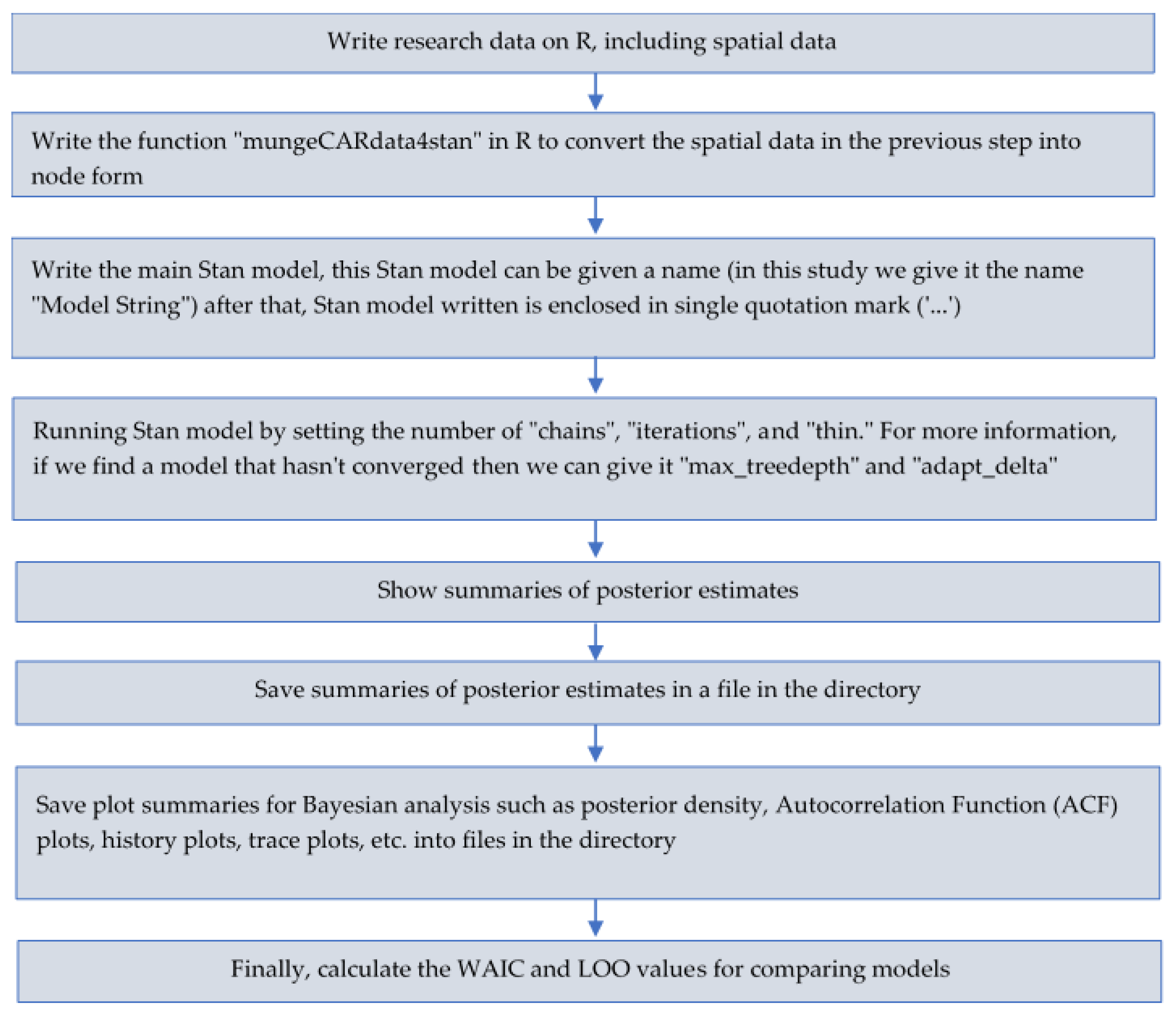
The development of Stan with the R interface (RStan) in this study is represented as the steps for modeling given in Figure 1.

6.1. Scotland Lip Cancer Dataset

This Scotland lip cancer dataset first discussed in Clayton and Kaldor [45] and Morris et al. [32] is also available in the GeoBUGS example in the OpenBUGS software (https://www.mrc-bsu.cam.ac.uk/software/bugs/the-bugs-project-the-bugs-book/bugs-book-examples/). The data include observed and expected cases (expected numbers based on the population and age and sex distribution in a county), a covariate measuring the percentage of the population engaged in agriculture, fishing, or forestry, and the "position’’ of each county expressed as a list of adjacent counties. For the lip cancer example, the model may be written as follows:

$$O_i\sim \mathrm{Poisson}\left({\mu }_i\right)$$

(16)

where $\log {\mu }_i=\log E_i+{\beta }_0+{\beta }_1\frac{x_i}{10}+{\varphi }_i$, where ${\varphi }_i$ is a spatial random effect.

To make our research applicable, we included a complete syntax for modeling the lip cancer dataset using the FSSN CAR model in the R interface (RStan) according to the steps in Figure 1. However, we divided this syntax into four partitions to make it easier, namely, Listing 3, Listing 4, Listing 5, and Listing 6. We created this syntax based on the BUGS syntax on the website that we listed above. There were two steps to doing so: Firstly, to install the Stan program on the R Interface (RStan), as can be seen on the following website: https://github.com/stan-dev/rstan/wiki/Installing-RStan-from-source-on-Windows. Secondly, we had to install the R packages, i.e., “rstan”, “ggplot2”, “StanHeaders”, “coda”, “dplyr”, “ggmcmc”, “shinystan”, “shiny”, and “loo”, in order to run this syntax. The following is an explanation for Listing 3: “O”, “E”, and “x” are filled with non-spatial research data, "num" is filled with the number of neighbors in each area, “adj” is filled with a list of neighbors from each area, “weights” is filled with the number 1, as many as the number of neighbors according to the fields in “adj”. Listing 4 provides information about the “mungeCARdata4stan” function, which is used to convert the spatial data in Listing 3 into node form. Listing 5 is the full code for the FSSN CAR model in Stan, where the FSSN distribution and FSSN CAR are provided in Listing 1 and Listing 2, respectively. Listing 6 is a step for running Stan’s program, displaying the summaries, saving the summaries in the directory, saving the plot of the posterior summaries, and finally, calculating the WAIC and LOO values.

Listing 3. Writing research data on R as written in the Bayesian inference using Gibbs sampling (BUGS) program.

#-----Research Data Including Spatial Data-----  data = list(S = 56,           O = c(9, 39, 11, 9, 15, 8, 26, …),           E = c( 1.4, 8.7, 3.0, 2.5, 4.3, 2.4, 8.1, …),           x = c(16,16,10,24,10,24,10, …),           num = c(4, 2, …),           adj = c( 5,9,11,19,                 7,10,                 …),           weights = c( 1,1,1,1,                   1,1,                     …)           )

Listing 4. The “mungeCARdata4stan” function is used to convert spatial data into nodes form.

#-----Function for Rewriting Spatial Data into Node Form-----   mungeCARdata4stan =function(adjBUGS, numBUGS){    S = length (numBUGS);    ss = numBUGS;    S_edges = length (adjBUGS)/ 2;    node1 = vector (mode="numeric", length=S_edges);    node2 = vector (mode="numeric", length=S_edges);    iAdj = 0;    iEdge = 0;    for(i in 1:S ){     for(j in 1:ss[i]){      iAdj = iAdj + 1;      if(i < adjBUGS[iAdj]){       iEdge = iEdge + 1;       node1[iEdge]= i;       node2[iEdge]= adjBUGS[iAdj];      }     }   }   return (list("S"=S,"S_edges"=S_edges,"node1"=node1,"node2"=node2));  }     #-----Calling Variables Used for Spatial-----  options(mc.cores = parallel::detectCores())     nbs = mungeCARdata4stan(data$adj, data$num);  S = data$S;              #Number of Areas  node1 = nbs$node1;  node2 = nbs$node2;  S_edges = nbs$S_edges;  O = data$O;  x = data$x;  E = data$E;     #-----Writing a List of Data-----  data.list =  list(O=O,E=E,x=x,S=S,S_edges=S_edges,node1=node1,node2=node2)  str(data.list)

Listing 5. The full syntax FSSN CAR model in Stan.

#-----Stan Model------  modelString=’  functions{    real FSSN_lpdf(real x, real mu, real sigma, real delta){     …    }    real car_FSSN_lpdf(vector phi, int N, int[[] node1, int[[]node2, real delta){    …        }    }  }  data {   int<lower=0> S;   int<lower=0> O[S];   vector<lower=0> [S] E;   vector<lower=0> [S] x;   int<lower=0> S_edges;   int<lower=1, upper=S> node1[S_edges]; // node1[i] adjacent to node2[i]   int<lower=1, upper=S> node2[S_edges]; // and node1[i] < node2[i]  }  parameters {   real alpha0;   real alpha1;   vector[S] fi;   real<lower=0> delta;  }  model {   alpha0~normal(0,1);   alpha1~normal(0,1);   delta~gamma(1,1);   fi~car_FSSN(S,node1,node2,delta);      for (i in 1:S)   O[i]~poisson(exp(log(E[i])+alpha0+alpha1*x[i]/10+fi[i]));  }  generated quantities {   vector[S] log_lik;    for (i in 1:S)    log_lik[i]       =       poisson_lpmf(O[i]       |  exp(log(E[i])+alpha0+alpha1*x[i]/10+fi[i]));  }  ’

Listing 6. Running Stan program, displays the summaries along with graph plots, and calculates WAIC and LOO values. Operator “::” defines the declaration for each function in each package.

#-----Running Stan Model----- rstan::stan_model rstan::stan   stanDso = stan_model(model_code=modelString) stanFit = stan( model_code=modelString, data=data.list, chains=4, iter=2000, thin=1, control=list(max_treedepth=20,adapt_delta=0.99))   #-----Display Summary----- base::summary   Summaries = summary(stanFit) Summaries   #-----Save Summary----- utils::capture.output   ofile = "D:/Output.txt"; capture.output(print(Summaries$summary, digits=3, probs=c(0.025, 0.975)),file=ofile,options(max.print =. Machine$integer.max))   #-----Display the Plot Summary----- coda::mcmc.list coda::mcmc ggmcmc:ggs ggmcmc::ggmcmc   stan2coda =function(stanFit){  mcmc.list(lapply(1:ncol(stanFit), function(X) mcmc(as.array(stanFit)[,X,])))} fit.mcmc = stan2coda(stanFit) ggso = ggs(fit.mcmc) ggmcmc(ggso,file=(paste("D:/Output.pdf")))   #-----Calculating WAIC----- loo::extract_log_lik loo::waic loo::loo   log_lik_1 = extract_log_lik(stanFit, parameter_name = "log_lik", merge_chains =TRUE) waic(log_lik_1) loo(log_lik_1)

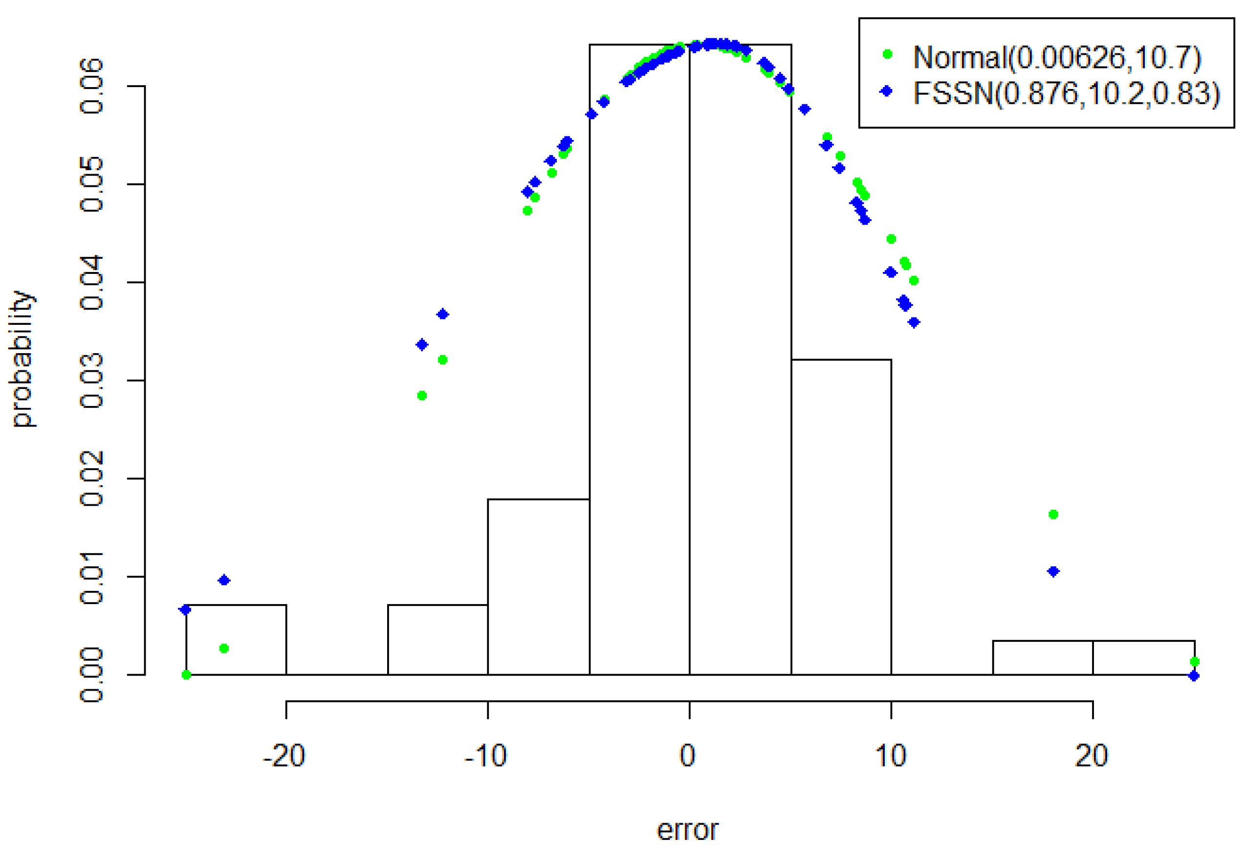
Model 1_Lip was set as Model 1 as the first step of “STEPS A” and applied to the Scotland lip cancer dataset. The parameter estimation results for Model 1_Lip are established in

Table 8. Estimated Model 1_Lip.

Parameters	Mean	semean	Std Dev	HPD Interval			neff	$\widehat{\mathbf{R}}$
				2.5%	50%	97.5%
${\beta }_0$	−0.5420	0.0012	0.0708	−0.6820	−0.5420	−0.4040	3264	1.0000
${\beta }_1$	0.7350	0.0011	0.0602	0.6150	0.7360	0.8530	3240	1.0000

. The term “se_mean” is the Monte Carlo standard error and “std dev” is the posterior standard deviation [46]. The term “n_eff” in the last two columns of Table 8 shows a crude measure of the effective sample size, and “$\hat{\mathrm{R}}$” elaborates the potential scale reduction factor on split chains. At convergence, the $\hat{\mathrm{R}}$ would be equal to 1 (see Carpenter et al. [47]), meaning that Model 1_Lip has reached convergence; the error patterns of both approximated normal and FSSN distributions are shown in Figure 2.

The error histogram of Model 1_Lip in Figure 2 shows that there are errors whose values are far distorted on the left. This can be covered by the FSSN distribution, but not for the normal distribution. This was the first indication that the FSSN CAR model is able to accommodate the spatial effects in the Scotland lip cancer dataset.

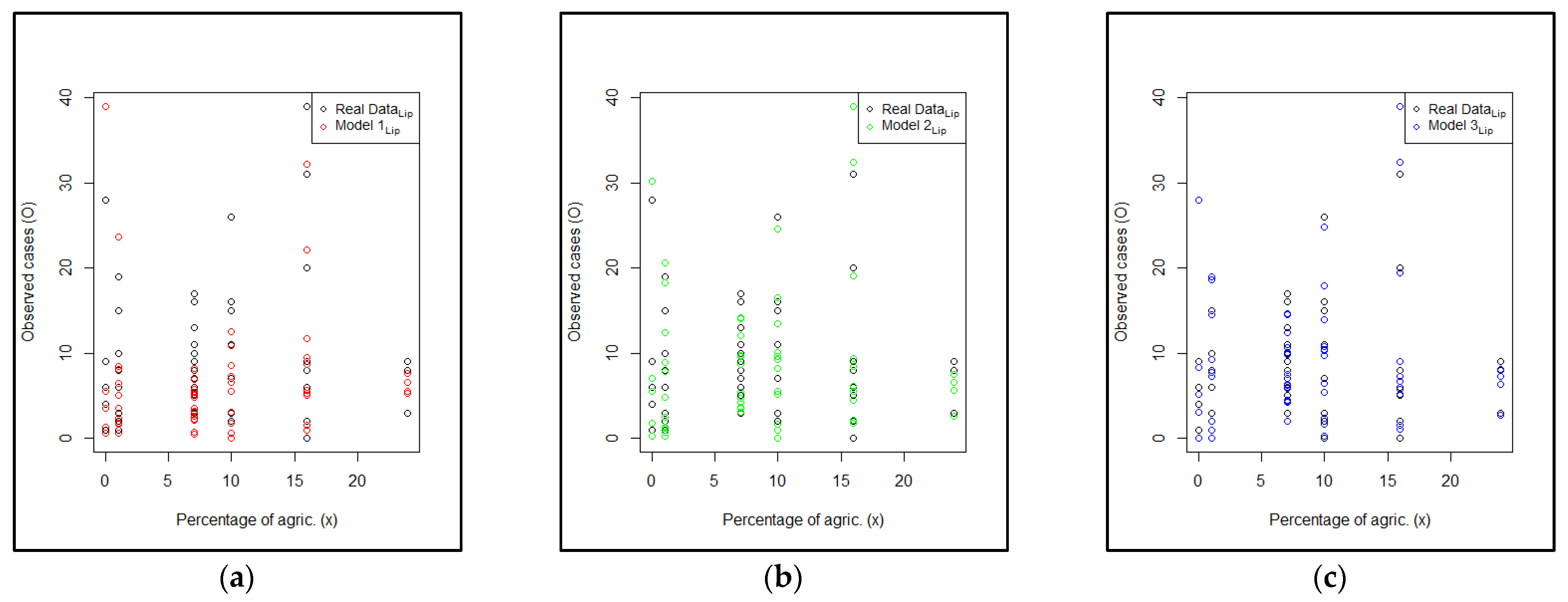
The next step was to set Model 2_Lip as Model 2, which was built by including the normal CAR spatial effect, and to set Model 3_Lip as Model 3, which was built by including the FSSN CAR spatial effect. The estimation parameters of Model 2_Lip and Model 3_Lip are given in

Table 9. Estimated Model 2_Lip.

Parameters	Mean	semean	Std Dev	HPD Interval			neff	$\widehat{\mathbf{R}}$
				2.5%	50%	97.5%
${\beta }_0$	−0.1732	0.0029	0.1410	−0.4541	−0.1707	0.1007	2320	1.0000
${\beta }_1$	0.2973	0.0033	0.1510	0.0049	0.2968	0.5967	2041	1.0000
${\varphi }_1$	1.2966	0.0033	0.3150	0.6451	1.3096	1.8945	8953	1.0000
${\varphi }_2$	1.1695	0.0028	0.1950	0.7873	1.1717	1.5513	4784	1.0000
$\cdots$	$\cdots$	$\cdots$	$\cdots$	$\cdots$	$\cdots$	$\cdots$	$\cdots$	$\cdots$
${\varphi }_{56}$	−0.5466	0.0035	0.3810	−1.2947	−0.5423	0.1808	11,606	1.0000

and

Table 10. Estimated Model 3_Lip.

Parameters	Mean	semean	Std Dev	HPD Interval			neff	$\widehat{\mathbf{R}}$
				2.5%	50%	97.5%
${\beta }_0$	−0.3136	0.0051	0.1950	−0.6937	−0.3146	0.0685	1440	1.0000
${\beta }_1$	0.3357	0.0058	0.2124	0.0838	0.3368	0.7456	1331	1.0000
${\varphi }_1$	1.3822	0.0041	0.3209	0.7380	1.3912	1.9960	6043	1.0000
${\varphi }_2$	1.2489	0.0046	0.2289	0.8046	1.2490	1.6959	2467	1.0000
$\cdots$	$\cdots$	$\cdots$	$\cdots$	$\cdots$	$\cdots$	$\cdots$	$\cdots$	$\cdots$
${\varphi }_{56}$	−0.8360	0.0078	0.7391	−2.4176	−0.7870	0.4737	9094	1.0000
${\delta }_1$	1.0019	0.0010	0.0996	0.8077	1.0009	1.1967	10,114	1.0000
${\delta }_2$	1.0034	0.0010	0.1018	0.8043	1.0021	1.2032	10,434	1.0000
$\cdots$	$\cdots$	$\cdots$	$\cdots$	$\cdots$	$\cdots$	$\cdots$	$\cdots$	$\cdots$
${\delta }_{56}$	0.9982	0.0010	0.0995	0.8035	0.9982	1.1972	10,039	1.0000

, respectively. The accuracy of the three models with respect to the original Scotland lip cancer dataset can be seen in Figure 3.

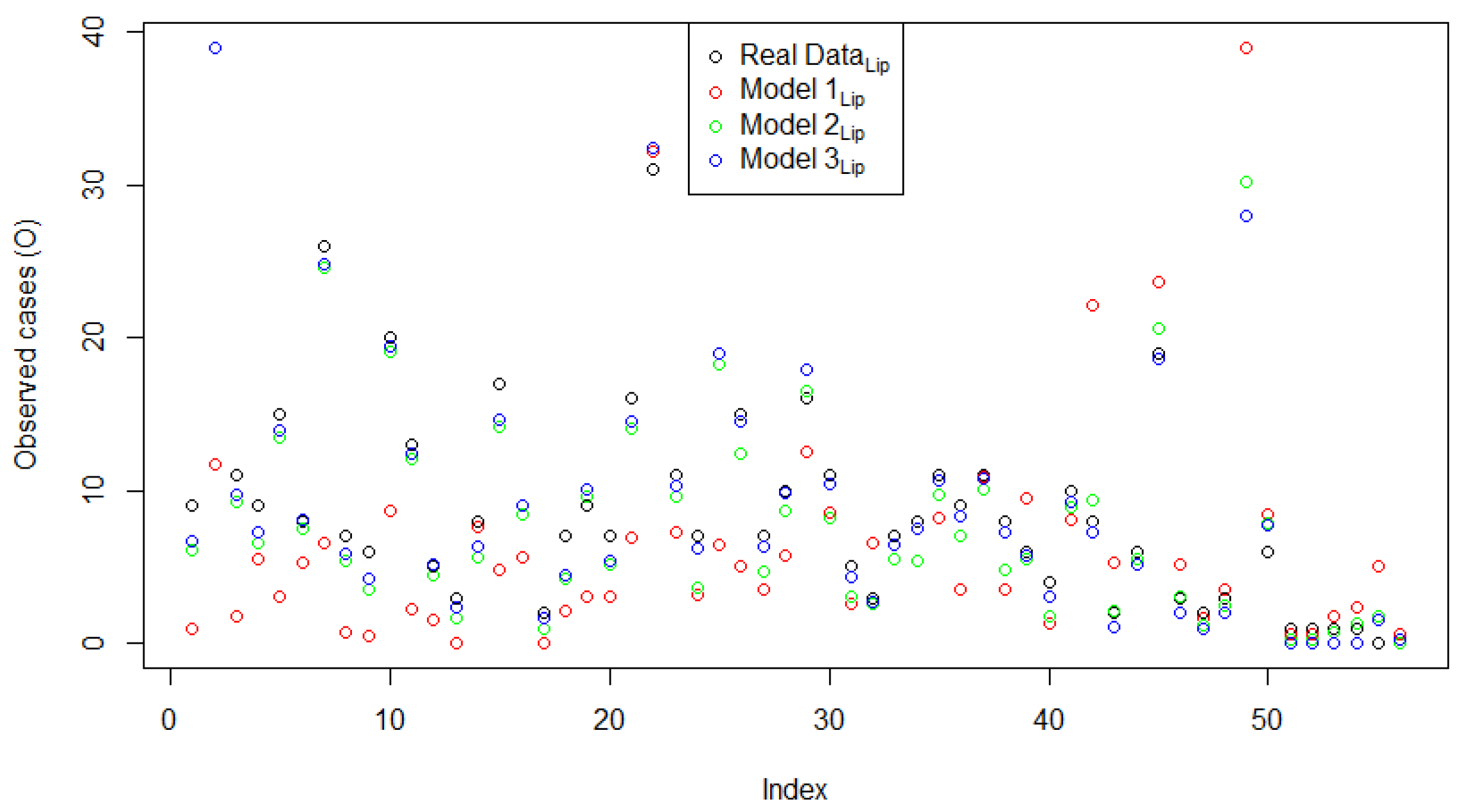
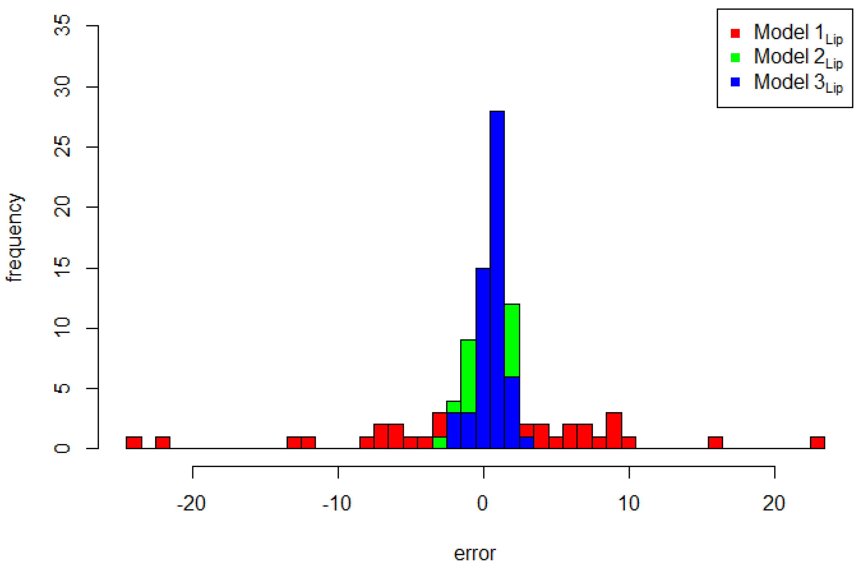
Figure 3 shows the plot of the explanatory variable versus the original response data compared to the predicted value of the three models. Model 3_Lip was closer to the original data than Model 1_Lip and Model 2_Lip. This means that the FSSN CAR model can catch error patterns better than the normal CAR model. To support this assertion, Figure 4 demonstrates three plots of the original response data and their predicted values based on the order of observation. Throughout the range of datasets, the predictive value of Model 3_Lip dominated in terms of its proximity to the original data. The comparison of the histograms of errors for all three models is given in Figure 5. The goodness of the three models, presented by the histogram in Figure 5, exhibits a very significant difference, with Model 3_Lip showing the smallest error variability.

A visual comparison of the models is given in Figure 3, Figure 4 and Figure 5. Then, we evaluated each model by their WAIC and LOO values, as shown in

Table 11. The widely applicable information criterion (WAIC) and leave-one-out (LOO) values for Model 1_Lip, Models 2_Lip, and Model 3_Lip.

Model	WAIC	LOO
Model 1Lip	460.9	460.9
Model 2Lip	290.1	305.6
Model 3Lip	288.0	303.5

, to compare the models.

Table 11 provides additional evidence of the goodness of fit of Model 3_Lip, which was very significant compared to the other two models. Considering both the WAIC and LOO values, Model 3_Lip presented the smallest values. On the basis of these facts, the FSSN CAR model statistically presented the most representative model when describing the Scotland lip cancer dataset.

6.2. Lung Cancer Dataset in a London Health Authority

For the second implementation example, we used a published lung cancer dataset as a standard example for spatial modeling. This dataset is available in GeoBUGS example on OpenBUGS software (https://www.mrc-bsu.cam.ac.uk/software/bugs/the-bugs-project-the-bugs-book/bugs-book-examples/). The data were simulated, observed, and expected the counts of lung cancer incidence in males aged 65 and over living in the London Health Authority region; the award level index of socio-economic deprivation is also available in Thomas et al. [18].

In this case, the model can be written as Equation (16), where $\log {\mu }_i=\log E_i+{\beta }_0+{\beta }_1{x}_i+h_i+{\varphi }_i,$ where ${\varphi }_i$ is the spatial random effects assigned as a CAR prior distribution, and the random effects are $h_i$, for which an exchangeable normal prior distribution is assumed. The random effect for each area is thus the sum of a spatially structured component ${\varphi }_i$ and an unstructured component $h_i$. This is termed a convolution prior, as can be seen in Besag et al. [48] and Mollie [49]. In the second application, the lung cancer dataset in a London Health Authority was employed. Analysis of this dataset would still use the syntax for analyzing the Scotland lip cancer dataset by changing the data input and changing the appropriate model.

Model 1_Lung was set as Model 1, as previously explained in STEPS A, and applied to the lung cancer dataset. Based on STEPS A, the analysis step for the lung cancer dataset was the same step as that of the lip cancer dataset analysis. Estimation results for the regression parameters and the second random effects in Model 1_Lung can be seen in

Table 12. Estimated Model 1_Lung.

Parameters	Mean	semean	Std Dev	HPD Interval			neff	$\widehat{\mathbf{R}}$
				2.5%	50%	97.5%
${\beta }_0$	−0.2430	0.0018	0.1155	−0.4802	−0.2387	−0.0252	4107	1.0000
${\beta }_1$	0.0500	0.0003	0.0213	0.0089	0.0498	0.0937	4994	1.0000
$h_1$	−0.1300	0.0027	0.2509	−0.6656	−0.1129	0.3352	8597	1.0000
$h_2$	−0.0650	0.0021	0.2271	−0.5439	−0.0555	0.3679	11,583	1.0000
$\cdots$	$\cdots$	$\cdots$	$\cdots$	$\cdots$	$\cdots$	$\cdots$	$\cdots$	$\cdots$
$h_{44}$	0.0410	0.0021	0.2363	−0.4393	0.0365	0.5167	12,192	1.0000

. The error pattern is shown in Figure 6.

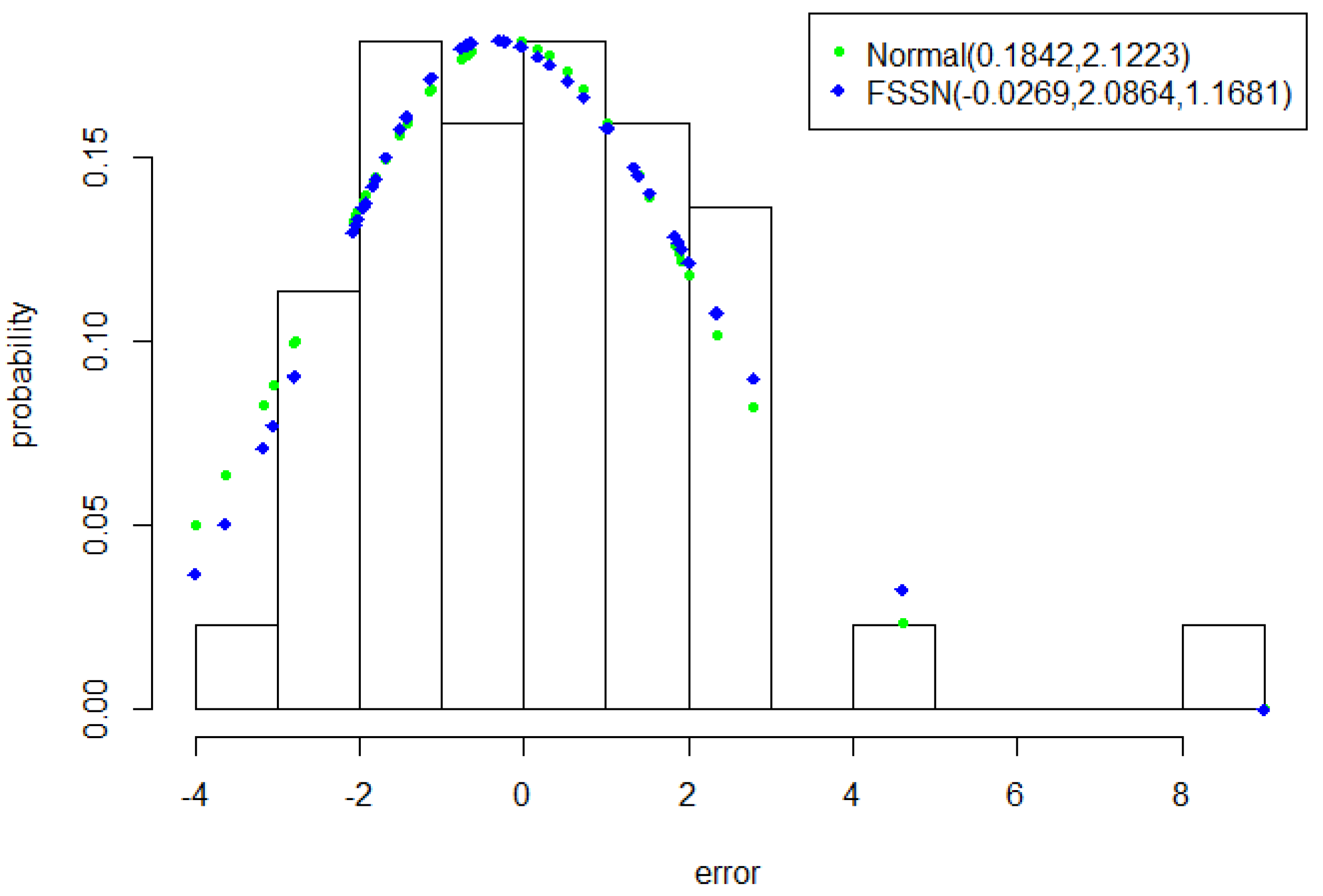
The Scotland lip cancer dataset has already helped to validate the FSSN distribute by demonstrating its ability to detect skew-left data. Figure 6 shows that the Model 1_Lung error had a skew-right shape. This fact provides an opportunity for the FSSN distribution to demonstrate its ability to detect the skewness of the error in the opposite direction and also challenges the normal distribution to demonstrate its ability to explain this error in a data-driven manner. The FSSN distribution was able to correctly estimate a skewness parameter of more than one; i.e., $\delta$ = 1.1681.

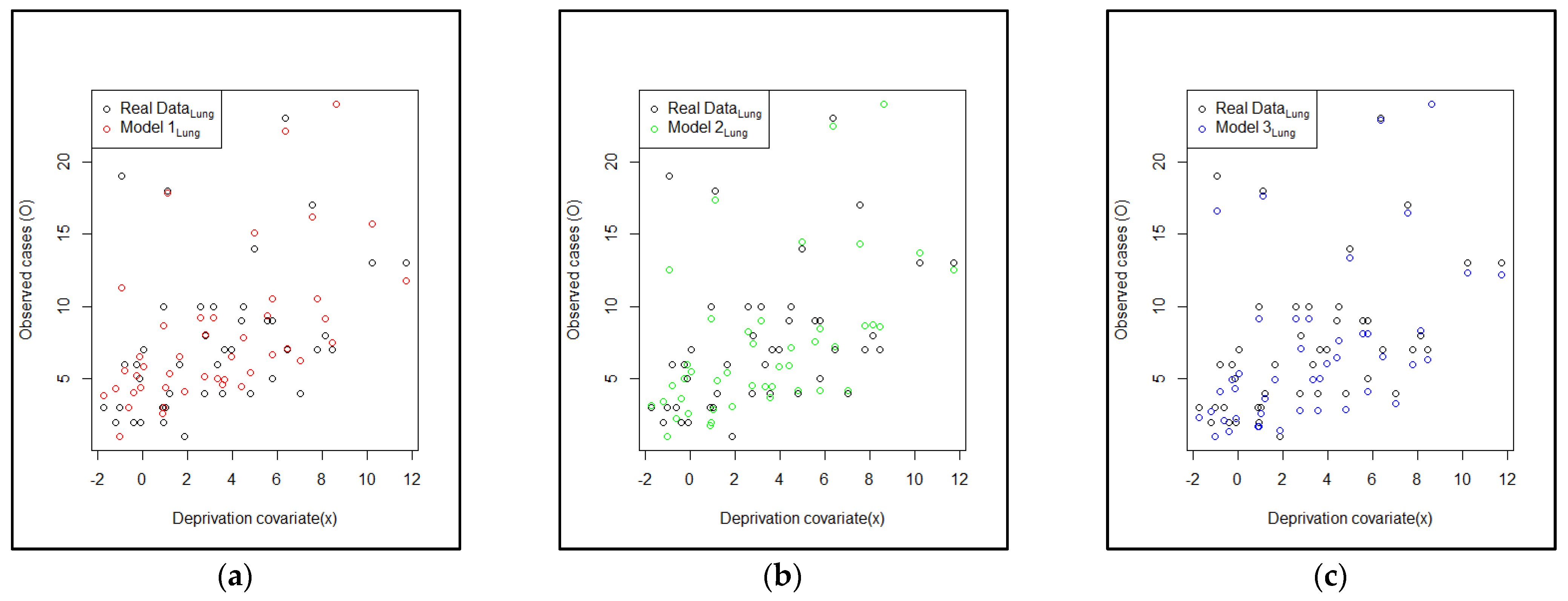
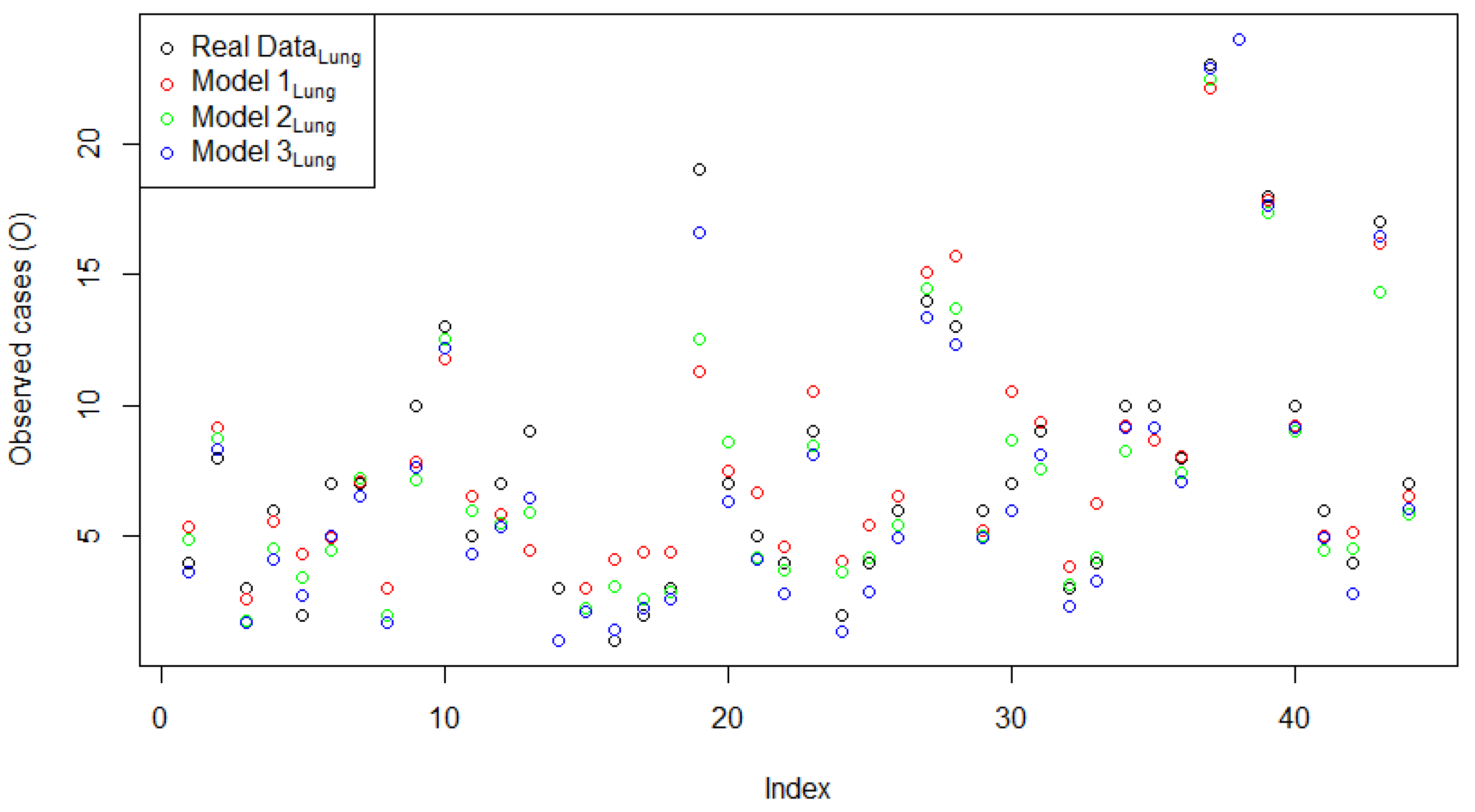
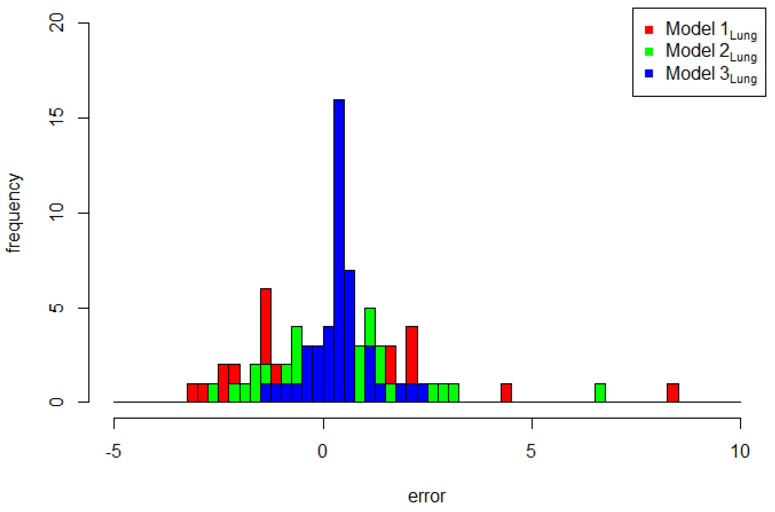
Next, the comparison of the two models with the normal CAR spatial effect (Model 2_Lung) and with the FSSN CAR spatial effect (Model 3_Lung) was obtained based on the estimated models in

Table 13. Estimated Model 2_Lung.

Parameters	Mean	semean	Std Dev				neff	$\widehat{\mathbf{R}}$
				2.5%	50%	97.5%
${\beta }_0$	−0.2340	0.0012	0.1397	−0.5115	−0.2340	0.0374	13,570	1.0000
${\beta }_1$	0.0340	0.0003	0.0345	−0.0333	0.0340	0.1015	11,639	1.0000
$h_1$	−0.0190	0.0009	0.1619	−0.4045	−0.0050	0.3141	34,365	1.0000
$h_2$	−0.0280	0.0012	0.1635	−0.4234	−0.0090	0.2898	19,422	1.0000
$\cdots$	$\cdots$	$\cdots$	$\cdots$	$\cdots$	$\cdots$	$\cdots$	$\cdots$	$\cdots$
$h_{44}$	0.0190	0.0009	0.1618	−0.3107	0.0050	0.3995	35,804	1.0000
${\varphi }_1$	−0.2610	0.0018	0.3451	−0.9488	−0.2560	0.3985	37,061	1.0000
${\varphi }_2$	0.0970	0.0020	0.3316	−0.5641	0.1010	0.7374	27,526	1.0000
$\cdots$	$\cdots$	$\cdots$	$\cdots$	$\cdots$	$\cdots$	$\cdots$	$\cdots$	$\cdots$
${\varphi }_{44}$	0.0260	0.0014	0.3024	−0.5850	0.0322	0.6043	47,473	1.0000

and

Table 14. Estimated Model 3_Lung.

Parameters	Mean	semean	Std Dev	HPD Interval			neff	$\widehat{\mathbf{R}}$
				2.5%	50%	97.5%
${\beta }_0$	−0.3412	0.0092	0.2091	−0.7600	−0.3400	0.0619	514.5	1.0100
${\beta }_1$	0.0509	0.0026	0.0554	−0.0570	0.0507	0.1601	3449.0	1.0100
$h_1$	−0.0412	0.0067	0.2582	−0.6223	−0.0138	0.4917	1505.6	1.0000
$h_2$	−0.0780	0.0076	0.2553	−0.6864	−0.0330	0.4014	1122.5	1.0100
$\cdots$	$\cdots$	$\cdots$	$\cdots$	$\cdots$	$\cdots$	$\cdots$	$\cdots$	$\cdots$
$h_{44}$	−0.0099	0.0102	0.2934	−0.6708	−0.0012	0.6140	3835.2	1.0000
${\varphi }_1$	−0.1937	0.0087	0.3713	−0.9347	−0.1870	0.5203	3820.3	1.0000
${\varphi }_2$	0.1120	0.0124	0.3903	−0.6733	0.1170	0.8737	3996.1	1.0100
$\cdots$	$\cdots$	$\cdots$	$\cdots$	$\cdots$	$\cdots$	$\cdots$	$\cdots$	$\cdots$
${\varphi }_{44}$	0.1750	0.0123	0.4822	−0.8131	0.1880	1.1019	3543.4	1.0000
${\delta }_1$	0.9992	0.0014	0.0997	0.8037	0.9990	1.1971	5045.0	1.0000
${\delta }_2$	1.0004	0.0014	0.0995	0.8075	1.0000	1.1969	5083.9	1.0000
$\cdots$	$\cdots$	$\cdots$	$\cdots$	$\cdots$	$\cdots$	$\cdots$	$\cdots$	$\cdots$
${\delta }_{44}$	1.0038	0.00142	0.0981	0.8127	1.0000	1.1994	4799.9	1.0000

, respectively. The predicted model of the estimation results for the three models is plotted in Figure 7. Three plots of the original response data and their predicted values based on the order of observation can be seen in Figure 8. It can be seen that the prediction of Model 3_Lung was the closest to the original data. In line with the evidence in Figure 8, Figure 9 reports the pattern of histogram errors of the three models, which also establishes that Model 3_Lung was the best model with the narrowest range of error variability.

The qualitative, descriptive, and visual presentation of the exploratory error needs to be continued by comparing the statistical criteria for model selection using WAIC and LOO values. These values can be seen in

Table 15. The WAIC and LOO values of Model 1_Lung, Model 2 _Lung, and Model 3 _Lung.

Model	WAIC	LOO
Model 1Lung	231.5	234.3
Model 2Lung	223.4	230.3
Model 3Lung	220.1	222.7

. Based on this table, Model 3_Lung was observed to be the best model due to it having the smallest WAIC and LOO values compared to the others. Once again, this lung cancer dataset also provided evidence that the FSSN CAR model has the ability to capture the phenomenon of skewed data.

7. Conclusions

An FSSN CAR model for analyzing spatial data is proposed in this paper. This approach was developed on the basis of the normal CAR model, which was given a skewness parameter to capture spatial data that has an asymmetrical pattern. The FSSN CAR model has demonstrated its capability to detect symmetric and asymmetric data patterns. Moreover, this model allows for the use of light- or heavy-tailed data. In real life, data that are truly symmetrical are rarely found. Thus, the FSSN distribution has a wide opportunity to be selected for analyzing data that has an almost symmetrical pattern. With its flexibility, the FSSN CAR model is more representative for modeling spatial random effects when compared to the normal CAR model.

This paper provides a simulation of data with 24 scenarios. The first to eighth scenarios used simulated symmetrical data patterns which were normally distributed with different variances and sample sizes. Meanwhile, the ninth to sixteenth scenarios used simulated symmetrical data which were plausibly leptokurtic, such as having a double-exponential distribution with different dispersions and sample sizes. Then, the seventeenth to the twenty-fourth scenarios used simulated symmetrical data patterns which were Student-t distributed with different degrees of freedom. On the basis of the analysis of the 24 scenarios, the FSSN distribution exhibited its capability to detect the 24 scenarios perfectly. These 24 scenarios were simulation studies carried out with 500 replications, then, the estimation results for each replication formed a 95% HPD interval for each parameter. The HPD interval for the skewness parameter in the FFSN distribution for the 24 scenarios was close to 1, indicating that the generated data was symmetrical. This was consistent with the data patterns of the generated distribution, namely, the normal, double-exponential, and Student-t distributions. Thus, through this estimated skewness parameter, it can be concluded that the FSSN can estimate the data generated from a normal, double-exponential, or Student-t distribution. Moreover, this HPD interval showed its capability to cover the targeted parameter values for all scenarios. At each replication, we recorded the posterior parameter, so that across replications, we got posterior values for each parameter according to the number of replications. From these posterior values, we obtained the bias, RMSE, and CP values. The bias values were close to zero for the estimated parameters of the 24 scenarios, especially for the FSSN goodness-of-fit distribution for the generated normal, double-exponential, and Student-t distribution data. For the 24 scenarios, the RMSE for the estimated parameters of the FSSN distribution were close to zero. The CP of the estimated parameters of the FSSN distribution were more than or equal to the normal distribution. On the basis of the HPD, biases, RMSE, and CP for the estimated parameters of the FSSN distribution, we can finally draw the conclusion that the FSSN distribution is able to estimate and capture the characteristics of data which are normally, double-exponentially, or Student-t distributed.

In addition, we presented 8 scenarios for the multivariate case. To measure the goodness of the estimation results in each scenario, the Euclidean distance was used. On the basis of the simulation results, the Euclidean distance in the multivariate FSSN distribution was smaller than in the multivariate normal distribution. The results obtained in the univariate simulation with 24 scenarios and the multivariate simulation with 8 scenarios show that the FSSN distribution is able to estimate the generated data according to these scenarios. This fact is what we used to model the spatial effect with the normal CAR model and the FSSN CAR as an alternative model.

The application of the FSSN CAR model to Scotland lip cancer dataset and the lung cancer dataset from the London Health Authority was also carried out. In this study, the FSSN CAR model challenged the normal CAR model. To compare the normal CAR and FSSN CAR models for these datasets, we used a visual comparison, namely, a plot for the original data against the estimated models. Visually, it was found that the FSSN CAR model was closer to the original data when compared to the normal CAR model. Then, on the basis of the WAIC and LOO values, the Poisson regression model with the FSSN CAR model was also found to be better than the normal CAR model. Both these test data showed the ability of the FSSN CAR model to explain left- and right-skew patterns. In contrast, the normal CAR model was only able to accommodate symmetry patterns and short tails.

We believe that, when data have a spatial effect, the use of the FSSN CAR model should be recommended over the normal CAR model. This is because of its ability to capture various data patterns covering the weakness of the normal CAR model for use with symmetrical data with short tails only. However, for the parameter estimation, normal CAR and FSSN CAR models give almost the same results.

References

1. Banerjee, S.; Wall, M.M.; Carlin, B.P. Frailty Modeling for Spatially Correlated Survival Data, with Application to Infant Mortality in Minnesota. Biostatistics 2003, 4, 123–142. [Google Scholar] [CrossRef] [Green Version]
2. Darmofal, D. Bayesian Spatial Survival Models for Political Event Processes. Am. J. Pol. Sci. 2009, 53, 241–257. [Google Scholar] [CrossRef] [Green Version]
3. Rantini, D.; Candrawengi, N.L.P.I.; Iriawan, N.; Irhamah; Rusli, M. On the Computational Bayesian Survival Spatial DHF Modelling with CAR Frailty. AIP Conf. Proc. 2021, 2329, 60028. [Google Scholar] [CrossRef]
4. Cressie, N.; Wikle, C.K. Statistics for Spatio-Temporal Data; John Wiley and Sons: Hoboken, NJ, USA, 2015. [Google Scholar]
5. Iriawan, N.; Astutik, S.; Prastyo, D.D. Markov Chain Monte Carlo—Based Approaches for Modeling the Spatial Survival with Conditional Autoregressive (CAR) Frailty. Int. J. Comput. Sci. Netw. Secur. 2010, 10, 211–217. [Google Scholar]
6. Aswi, A.; Cramb, S.; Duncan, E.; Hu, W.; White, G.; Mengersen, K. Bayesian Spatial Survival Models for Hospitalisation of Dengue: A Case Study of Wahidin Hospital in Makassar, Indonesia. Int. J. Environ. Res. Public Health 2020, 17, 878. [Google Scholar] [CrossRef] [PubMed] [Green Version]
7. Motarjem, K.; Mohammadzadeh, M.; Abyar, A. Bayesian Analysis of Spatial Survival Model with Non-Gaussian Random Effect. J. Math. Sci. 2019, 237, 692–701. [Google Scholar] [CrossRef]
8. Rantini, D.; Iriawan, N.; Irhamah. Bayesian Mixture Generalized Extreme Value Regression with Double-Exponential CAR Frailty for Dengue Haemorrhagic Fever in Pamekasan, East Java, Indonesia. J. Phys. Conf. Ser. 2021, 1752, 12022. [Google Scholar] [CrossRef]
9. Rantini, D.; Abdullah, M.N.; Iriawan, N.; Irhamah; Rusli, M. On the Computational Bayesian Survival Spatial Dengue Hemorrhagic Fever (DHF) Modeling with Double-Exponential CAR Frailty. J. Phys. Conf. Ser. 2021, 1722, 012042. [Google Scholar] [CrossRef]
10. Mbalawata, I.S.; Särkkä, S.; Haario, H. Parameter Estimation in Stochastic Differential Equations with Markov Chain Monte Carlo and Non-Linear Kalman Filtering. Comput. Stat. 2013, 28, 1195–1223. [Google Scholar] [CrossRef]
11. Duane, S.; Kennedy, A.D.; Pendleton, B.J.; Roweth, D. Hybrid Monte Carlo. Phys. Lett. B 1987, 195, 216–222. [Google Scholar] [CrossRef]
12. Neal, R.M. MCMC Using Hamiltonian Dynamics. In Handbook of Markov Chain Monte Carlo; Chapman and Hall: London, UK, 2011; pp. 113–162. [Google Scholar] [CrossRef] [Green Version]
13. Chen, T.; Fox, E.; Guestrin, C. Stochastic Gradient Hamiltonian Monte Carlo. In Proceedings of the International Conference on Machine Learning, PMLR, Beijing, China, 21–26 June 2014; pp. 1683–1691. [Google Scholar]
14. Fichtner, A.; Simutė, S. Hamiltonian Monte Carlo Inversion of Seismic Sources in Complex Media. J. Geophys. Res. Solid Earth 2018, 123, 2984–2999. [Google Scholar] [CrossRef]
15. Girolami, M.; Calderhead, B. Riemann Manifold Langevin and Hamiltonian Monte Carlo Methods. J. R. Stat. Soc. Ser. B Stat. Methodol. 2011, 73, 123–214. [Google Scholar] [CrossRef]
16. Betancourt, M.; Byrne, S.; Livingstone, S.; Girolami, M. The Geometric Foundations of Hamiltonian Monte Carlo. Bernoulli 2017, 23, 2257–2298. [Google Scholar] [CrossRef]
17. Livingstone, S.; Betancourt, M.; Byrne, S.; Girolami, M. On the Geometric Ergodicity of Hamiltonian Monte Carlo. Bernoulli 2019, 25, 3109–3138. [Google Scholar] [CrossRef] [Green Version]
18. Thomas, A.; Best, N.; Lunn, D.; Arnold, R.; Spiegelhalter, D. GeoBugs User Manual; Cambridge Medical Research Council Biostatistics Unit: Cambridge, UK, 2004. [Google Scholar]
19. Monnahan, C.C.; Thorson, J.T.; Branch, T.A. Faster Estimation of Bayesian Models in Ecology Using Hamiltonian Monte Carlo. Methods Ecol. Evol. 2017, 339–348. [Google Scholar] [CrossRef]
20. Annis, J.; Miller, B.J.; Palmeri, T.J. Bayesian Inference with Stan: A Tutorial on Adding Custom Distributions. Behav. Res. Methods 2017, 49, 863–886. [Google Scholar] [CrossRef] [PubMed] [Green Version]
21. Wetzels, R.; Lee, M.D.; Wagenmakers, E.J. Bayesian Inference Using WBDev: A Tutorial for Social Scientists. Behav. Res. Methods 2010, 42, 884–897. [Google Scholar] [CrossRef]
22. Wabersich, D.; Vandekerckhove, J. Extending JAGS: A Tutorial on Adding Custom Distributions to JAGS (with a Diffusion Model Example). Behav. Res. Methods 2014, 46, 15–28. [Google Scholar] [CrossRef] [Green Version]
23. Ghaderinezhad, F.; Ley, C.; Loperfido, N. Bayesian Inference for Skew-Symmetric Distributions. Symmetry 2020, 12, 491. [Google Scholar] [CrossRef] [Green Version]
24. Castillo, N.O.; Gómez, H.W.; Leiva, V.; Sanhueza, A. On the Fernández–Steel Distribution: Inference and Application. Comput. Stat. Data Anal. 2011, 55, 2951–2961. [Google Scholar] [CrossRef]
25. Azzalini, A. The Skew-Normal Distribution and Related Multivariate Families. Scand. J. Stat. 2005, 32, 159–188. [Google Scholar] [CrossRef]
26. Zhang, J.; Shields, M.D. On the Quantification and Efficient Propagation of Imprecise Probabilities Resulting from Small Datasets. Mech. Syst. Signal Process. 2018, 98, 465–483. [Google Scholar] [CrossRef]
27. Beer, M.; Ferson, S.; Kreinovich, V. Imprecise Probabilities in Engineering Analyses. Mech. Syst. Signal Process. 2013, 37, 4–29. [Google Scholar] [CrossRef] [Green Version]
28. Torre, E.; Marelli, S.; Embrechts, P.; Sudret, B. A General Framework for Data-Driven Uncertainty Quantification under Complex Input Dependencies Using Vine Copulas. Probabilistic Eng. Mech. 2019, 55, 1–16. [Google Scholar] [CrossRef] [Green Version]
29. Zhang, J.; Shields, M.D. Efficient Monte Carlo Resampling for Probability Measure Changes from Bayesian Updating. Probabilistic Eng. Mech. 2019, 55, 54–66. [Google Scholar] [CrossRef]
30. Zhang, J.; Shields, M. On the Quantification and Efficient Propagation of Imprecise Probabilities with Copula Dependence. Int. J. Approx. Reason. 2020, 122, 24–46. [Google Scholar] [CrossRef]
31. Fernández, C.; Steel, M.F.J. On Bayesian Modeling of Fat Tails and Skewness. J. Am. Stat. Assoc. 1998, 93, 359–371. [Google Scholar] [CrossRef] [Green Version]
32. Morris, M.; Wheeler-Martin, K.; Simpson, D.; Mooney, S.J.; Gelman, A.; DiMaggio, C. Bayesian Hierarchical Spatial Models: Implementing the Besag York Mollié Model in Stan. Spat. Spatiotempor. Epidemiol. 2019, 31, 1–18. [Google Scholar] [CrossRef] [PubMed]
33. Besag, J. Spatial Interaction and the Statistical Analysis of Lattice Systems. J. R. Stat. Soc. Ser. B 1974, 36, 192–225. [Google Scholar] [CrossRef]
34. Banerjee, S.; Carlin, B.P.; Gelfand, A.E. Hierarchical Modeling and Analysis for Spatial Data; Chapman and Hall: London, UK, 2014. [Google Scholar]
35. Ferreira, J.T.A.S.; Steel, M.F.J. A New Class of Skewed Multivariate Distributions with Applications to Regression Analysis. Stat. Sin. 2007, 17, 505–529. [Google Scholar]
36. Walther, B.A.; Moore, J.L. The Concepts of Bias, Precision and Accuracy, and Their Use in Testing the Performance of Species Richness Estimators, with a Literature Review of Estimator Performance. Ecography 2005, 28, 815–829. [Google Scholar] [CrossRef]
37. Andronescu, M.; Condon, A.; Hoos, H.H.; Mathews, D.H.; Murphy, K.P. Computational Approaches for RNA Energy Parameter Estimation. RNA 2010, 16, 2304–2318. [Google Scholar] [CrossRef] [Green Version]
38. Zhao, H.; Tian, L. On Estimating Medical Cost and Incremental Cost-Effectiveness Ratios with Censored Data. Biometrics 2001, 57, 1002–1008. [Google Scholar] [CrossRef]
39. Hitchcock, S.; Hogg, R.V.; Craig, A.T. Introduction to Mathematical Statistics; Pearson Education: London, UK, 1966; Volume 129. [Google Scholar] [CrossRef]
40. Dokmanic, I.; Parhizkar, R.; Ranieri, J.; Vetterli, M. Euclidean Distance Matrices: Essential Theory, Algorithms, and Applications. IEEE Signal Process. Mag. 2015, 32, 12–30. [Google Scholar] [CrossRef] [Green Version]
41. Lele, S. Euclidean Distance Matrix Analysis (EDMA): Estimation of Mean Form and Mean Form Difference. Math. Geol. 1993, 25, 573–602. [Google Scholar] [CrossRef]
42. Lax, P.D. Linear Algebra and Its Applications, 2nd ed.; John Wiley and Sons: Hoboken, NJ, USA, 2013. [Google Scholar]
43. Watanabe, S. Asymptotic Equivalence of Bayes Cross Validation and Widely Applicable Information Criterion in Singular Learning Theory. J. Mach. Learn. Res. 2010, 11, 3571–3594. [Google Scholar]
44. Vehtari, A.; Gelman, A.; Gabry, J. Practical Bayesian Model Evaluation Using Leave-One-out Cross-Validation and WAIC. Stat. Comput. 2017, 27, 1413–1432. [Google Scholar] [CrossRef] [Green Version]
45. Clayton, D.; Kaldor, J. Empirical Bayes Estimates of Age-Standardized Relative Risks for Use in Disease Mapping. Biometrics 1987, 43, 671–681. [Google Scholar] [CrossRef] [PubMed]
46. Gelman, A.; Lee, D.; Guo, J. Stan: A Probabilistic Programming Language for Bayesian Inference and Optimization. J. Educ. Behav. Stat. 2015, 20, 1–14. [Google Scholar] [CrossRef] [Green Version]
47. Carpenter, B.; Gelman, A.; Hoffman, M.D.; Lee, D.; Goodrich, B.; Betancourt, M.; Brubaker, M.A.; Guo, J.; Li, P.; Riddell, A. Stan: A Probabilistic Programming Language. J. Stat. Softw. 2017, 76, 1–32. [Google Scholar] [CrossRef] [Green Version]
48. Besag, J.; York, J.; Mollié, A. Bayesian Image Restoration, with Two Applications in Spatial Statistics. Ann. Inst. Stat. Math. 1991, 43, 1–20. [Google Scholar] [CrossRef]
49. Mollié, A. Bayesian Mapping of Disease. Markov Chain Mt. Carlo Pract. 1996, 1, 359–379. [Google Scholar]
Figure 1. The steps for modeling using Stan in the R interface (RStan).
Symmetry 13 00545 g001
Figure 2. Plots of the error of Model 1Lip with approximated normal and Fernandez–Steel skew normal (FSSN) distributions.
Symmetry 13 00545 g002
Figure 3. Plots of the original data with the estimated model for (a) Model 1Lip, (b) Models 2Lip, and (c) Model 3Lip.
Symmetry 13 00545 g003
Figure 4. Plots of the original response data and predicted value for Model 1Lip, Models 2Lip, and Model 3Lip based on the observation order.
Symmetry 13 00545 g004
Figure 5. Error histogram plots of Model 1Lip, Model 2Lip, and Model 3Lip.
Symmetry 13 00545 g005
Figure 6. Plots of the Model 1Lung error histogram with approximated normal and FSSN distributions.
Symmetry 13 00545 g006
Figure 7. Plots of the original data with the estimated model: (a) Model 1Lung, (b) Model 2 Lung, and (c) Model 3 Lung.
Symmetry 13 00545 g007
Figure 8. Plots of the original response data and predicted value of Model 1Lung, Model 2 Lung, and Model 3 Lung based on the observation order.
Symmetry 13 00545 g008
Figure 9. Error histogram plots of Model 1Lung, Model 2 Lung, and Model 3 Lung.
Symmetry 13 00545 g009