A Chebyshev Wavelet Collocation Method for Some Types of Differential Problems

Abstract

In the past decade, various types of wavelet-based algorithms were proposed, leading to a key tool in the solution of a number of numerical problems. This work adopts the Chebyshev wavelets for the numerical solution of several models. A Chebyshev operational matrix is developed, for selected collocation points, using the fundamental properties. Moreover, the convergence of the expansion coefficients and an upper estimate for the truncation error are included. The obtained results for several case studies illustrate the accuracy and reliability of the proposed approach.

1. Introduction

Several algorithms, such as the finite difference and finite element, as well as spectral techniques, have been used in the approximation of mathematical models [1,2,3,4]. Nowadays, considerable attention is being paid to distinct types of wavelet methods to improve the formulation of mathematical models. Wavelets have relevant features such as orthogonality, capability of representing functions with different levels of resolution, and the exact representation of polynomials, just to mention a few. Such properties stimulated the development of efficient algorithms based on the Haar, Daubechies, and Legendre wavelets [5,6] that lead to highly stable results [7,8].

The Galerkin and collocation approaches along with wavelets [9,10,11,12] were applied in elasticity problems. For the case of the Haar wavelets, we can mention the work of Lepik et al. [13]. Some special classes of boundary value problems (BVPs), such as the Lane–Emden and Bratu’s type equations, were analyzed by Abd-Elhameed et al. [14] using a wavelet collocation approach. Robertsson and Blanch [15] proposed the Galerkin wavelets as a numerical tool for handling the solution of partial differential equations (PDEs). Heydari et al. [16] addressed the telegraph and the second-order hyperbolic differential equations using Chebyshev wavelets. Vivek and Mehra [17] advanced a wavelet finite difference approach for solving self-adjoint singularly perturbed boundary value problems. Recently, Dhawan et al. [18,19,20] developed a computational scheme based on these methods.

It has been observed from the literature survey that wavelets are basically localized functions that are capable of producing accurate solutions [21,22]. Thus, the development of wavelet-based techniques allows a fast and efficient evaluation of the problems under consideration, while posing a low computational cost [23,24].

Having in mind the properties of wavelet methods, we propose a Chebyshev wavelet algorithm for solving some types of differential equations. Therefore, the manuscript is organized as follows: The fundamental definitions and the mathematical concepts required by the proposed algorithm are presented in Section 2. The application of the Chebyshev wavelets for solving the problems under analysis and the corresponding results are discussed in Section 3. Finally, the main conclusions are summarized in Section 4.

2. Fundamental Definitions and Mathematical Concepts

2.1. Chebyshev and Shifted Chebyshev Polynomials

The Chebyshev polynomials are defined in the interval $t\in [-1,1]$ and are obtained by expanding the formula [25,26,27]

$$T_n\left(t\right)=cos(narccos\left(t\right)),n=0,1,\cdots ,t\in [-1,1].$$

(1)

These polynomials follow recurrence relation

$$T_0\left(t\right)=1,T_1\left(t\right)=t,T_{m+1}\left(t\right)=2t{T}_m\left(t\right)-T_{m-1}\left(t\right),m=1,2,\cdots .$$

(2)

The analytic form of a Chebyshev polynomial of degree n is given by

$$T_n\left(t\right)=\sum _{i=0}^{[n/2]}(-1)2^{n-2i-1}\frac{n(n-i-1)!}{i!(n-2i)!}{t}^{n-2i},$$

(3)

and obeys the orthogonality condition

$${\int }_{-1}^1{T}_n\left(t\right)T_m\left(t\right)\frac{dt}{\sqrt{1-t^2}}=\left\{\begin{array}{cc}\pi ,\hfill & n=m=0,\hfill \\ \pi /2,\hfill & n=m\ne 0,\hfill \\ 0,\hfill & n\ne m.\hfill \end{array}\right.$$

We construct the shifted Chebyshev polynomials through the change of variable $t=2x-1$. Therefore, the shifted Chebyshev polynomials ${\tilde{T}}_m\left(x\right)$, $x\in [0,1]$, can be obtained as ${\tilde{T}}_m\left(x\right)=T_m(2x-1)$ and we have ${\tilde{T}}_0\left(x\right)=1,{\tilde{T}}_1\left(x\right)=2x-1,{\tilde{T}}_{m+1}\left(x\right)=2(2x-1){\tilde{T}}_m\left(x\right)-T_{m-1}\left(x\right)$ for $m=1,2,\cdots$. The analytic form of the shifted Chebyshev polynomial of degree n can be expressed as: ${\tilde{T}}_n\left(t\right)={\sum }_{i=0}^n(-1)2^{2n-2i}\frac{n(2n-i-1)!}{i!(2n-2i)!}{x}^{n-i}$ and the orthogonality condition is formulated as

$${\int }_0^1\frac{{\tilde{T}}_m\left(x\right){\tilde{T}}_n\left(x\right)}{\sqrt{1-{(2x-1)}^2}}dx=\left\{\begin{array}{cc}\frac{\pi {\alpha }_m}{4},\hfill & m=n,\hfill \\ 0,\hfill & m\ne n,\hfill \end{array}\right.$$

(4)

where

$${\alpha }_m=\left\{\begin{array}{cc}2,\hfill & m=0,\hfill \\ 1,\hfill & m\ge 1.\hfill \end{array}\right.$$

(5)

The function $u\left(x\right)$, which is square Lebesgue integrable, can be written in terms of the shifted Chebyshev polynomials as

$$u\left(x\right)=\sum _{i=0}^{\infty }{c}_i\widetilde{T_i}\left(x\right),$$

(6)

where the coefficients $c_i,i=0,1,2,\cdots$, are given by

$$c_i=\frac{1}{\pi }{\int }_{-1}^1\frac{u(x+1)T_i\left(x\right)}{\sqrt{1-x^2}}dx.$$

2.2. The Chebyshev Wavelets

The wavelets represent a family of functions that are obtained by the means of dilation and translation of the mother wavelet $\varphi \left(x\right)$. When the dilation parameter and the translation parameters, s and t, respectively, vary, we obtain a family of continuous wavelets:

$$\begin{array}{c}\hfill {\varphi }_{s,t}\left(x\right)={\left|s\right|}^{-1/2}\varphi \left(\frac{x-t}{s}\right),s,t\in \mathbb{R},s\ne 0.\end{array}$$

(7)

As a matter of fact, orthogonal functions and polynomials are useful tools, and the Chebyshev wavelet technique has been successfully applied in several problems [7,8]. The key characteristic of this technique is that it reduces a given problem to a system of algebraic equations by means of a truncated approximation series

$$u\left(x\right)\simeq u_N\left(x\right)=\sum _{i=0}^{N-1}{l}_i{\varphi }_i\left(x\right),$$

(8)

where $l_i$ are the unknown expansion coefficients. The elements ${\varphi }_0\left(x\right),{\varphi }_1\left(x\right),...,{\varphi }_{N-1}\left(x\right)$ represent the orthonormal basis functions defined on a given interval $[a,b]$. Hereafter, we choose ${\varphi }_i\left(x\right)$ as Chebyshev wavelets on $x\in [0,1]$ given by

$$\begin{array}{c}\hfill {\varphi }_{n,m}=\left\{\begin{array}{cc}{2}^{\frac{k}{2}}{\tilde{T}}_m(2^{k}x-2n+1),\hfill & \frac{n-1}{2^{k-1}}\le x<\frac{n}{2^{k-1}},\hfill \\ 0,\hfill & \mathrm{otherwise},\hfill \end{array}\right.\end{array}$$

(9)

so that

$$\begin{array}{c}\hfill {\tilde{T}}_m=\left\{\begin{array}{cc}\frac{1}{\sqrt{\pi }},\hfill & m=0,\hfill \\ \sqrt{\frac{2}{\pi }}{T}_m\left(x\right),\hfill & m\ge 1,\hfill \end{array}\right.\end{array}$$

(10)

where $m=0,1,...,M$ and $n=0,...,2^k-1$. We also remark that the Chebyshev wavelets are an orthonormal set with weight function

$$\begin{array}{c}\hfill w_k\left(x\right)=\left\{\begin{array}{cc}{w}_{1,k}\left(x\right),\hfill & 0\le x<\frac{1}{2^{k-1}},\hfill \\ w_{2,k}\left(x\right),\hfill & \frac{1}{2^{k-1}}\le x<\frac{2}{2^{k-1}},\hfill \\ .\hfill & .\hfill \\ .\hfill & .\hfill \\ .\hfill & .\hfill \\ w_{2^{k-1},k}\left(x\right),\hfill & \frac{2^{k-1}-1}{2^{k-1}}\le x<1,\hfill \end{array}\right.\end{array}$$

where $w_{n,k}\left(x\right)=w(2^{k+1}x-2n-1)$.

By using the shifted Chebyshev polynomials in the interval $\frac{n-1}{2^{k-1}}\le x<\frac{n}{2^{k-1}}$, we have

$$\begin{array}{ccc}\hfill {\varphi }_{n,m}& =& \frac{2^{\frac{k-1}{2}}}{\sqrt{\pi }}{T}_m(2^{k}x-2n+1)\hfill \\ \hfill {\varphi }_{n,m}^{\prime }\left(x\right)& =& \left\{\begin{array}{cc}\frac{2^{\frac{k-1}{2}}}{\sqrt{\pi }}{2}^{k}2m\sum _{k=1}^{m-1}{T}_k(2^{k}x-2n+1),\hfill & \mathrm{when}m\mathrm{is}\mathrm{even}\hfill \\ \frac{2^{\frac{k-1}{2}}}{\sqrt{\pi }}{2}^k[2m\sum _{k=1}^{m-1}{T}_k(2^{k}x-2n+1)+m{T}_0(2^{k}x-2n+1)],\hfill & \mathrm{when}m\mathrm{is}\mathrm{odd}.\hfill \end{array}\right.\hfill \end{array}$$

For calculating the operational matrix of derivative, if we take $M=2$ and $k=2$, then we get

$$\begin{array}{ccc}& & {\varphi }_{1,0}=\left\{\begin{array}{cc}\frac{\sqrt{2}}{\sqrt{\pi }},\hfill & 0\le x<1/2,\hfill \\ 0,\hfill & \mathrm{otherwise},\hfill \end{array}\right.,\hfill \\ & & {\varphi }_{1,1}=\left\{\begin{array}{cc}\frac{\sqrt{2}}{\sqrt{\pi }}(4x-1),\hfill & 0\le x<1/2,\hfill \\ 0,\hfill & \mathrm{otherwise},\hfill \end{array}\right.,\hfill \\ & & {\varphi }_{1,2}=\left\{\begin{array}{cc}\frac{\sqrt{2}}{\sqrt{\pi }}(2{(4x-1)}^2-1),\hfill & 0\le x<1/2,\hfill \\ 0,\hfill & \mathrm{otherwise}\hfill \end{array}\right.,\hfill \\ & & {\varphi }_{1,3}=\left\{\begin{array}{cc}\frac{\sqrt{2}}{\sqrt{\pi }}(256x^3-192x^2+36x-1),\hfill & 0\le x<1/2,\hfill \\ 0,\hfill & \mathrm{otherwise},\hfill \end{array}\right.,\hfill \end{array}$$

$$\begin{array}{ccc}& & {\varphi }_{2,0}=\left\{\begin{array}{cc}\frac{\sqrt{2}}{\sqrt{\pi }},\hfill & 1/2\le x<1,\hfill \\ 0,\hfill & \mathrm{otherwise},\hfill \end{array}\right.,\hfill \\ & & {\varphi }_{2,1}=\left\{\begin{array}{cc}\frac{\sqrt{2}}{\sqrt{\pi }}(4x-3),\hfill & 1/2\le x<1,\hfill \\ 0,\hfill & \mathrm{otherwise}\hfill \end{array}\right.,\hfill \\ & & {\varphi }_{2,2}=\left\{\begin{array}{cc}\frac{\sqrt{2}}{\sqrt{\pi }}(2{(4x-3)}^2-1),\hfill & 1/2\le x<1,\hfill \\ 0,\hfill & \mathrm{otherwise},\hfill \end{array}\right.,\hfill \\ & & {\varphi }_{2,3}=\left\{\begin{array}{cc}\frac{\sqrt{2}}{\sqrt{\pi }}(256x^3-576x^2+420x-99),\hfill & 1/2\le x<1,\hfill \\ 0,\hfill & \mathrm{otherwise}.\hfill \end{array}\right.,\hfill \end{array}$$

Table 1 represents the calculated derivatives of ${\varphi }_{n,m}$ when $M=k=2$.

Table 1. The calculated derivatives of ${\varphi }_{n,m}$ when $M=k=2$.

${\mathit{\varphi }}_{1,0}^{\prime }$	${\mathit{\varphi }}_{1,1}^{\prime }$	${\mathit{\varphi }}_{1,2}^{\prime }$	${\mathit{\varphi }}_{1,3}^{\prime }$	${\mathit{\varphi }}_{2,0}^{\prime }$	${\mathit{\varphi }}_{2,1}^{\prime }$	${\mathit{\varphi }}_{2,2}^{\prime }$	${\mathit{\varphi }}_{2,3}^{\prime }$
0	$4\sqrt{2}{\varphi }_{1,0}$	$16{\varphi }_{1,1}$	$12\sqrt{2}+24{\varphi }_{1,2}{\varphi }_{1,0}$	0	$4\sqrt{2}{\varphi }_{2,0}$	$16{\varphi }_{2,1}$	$12\sqrt{2}{\varphi }_{2,0}+24{\varphi }_{2,3}$

The function ${\varphi }_i\left(x\right)$ is zero outside the interval $\frac{n-1}{2^{k-1}}\le x<\frac{n}{2^{k-1}}$, so that

$${\varphi }_i^{\prime }\left(x\right)=P{\varphi }_i\left(x\right),i=1,2,...,2^{k-1},$$

where

$$\begin{array}{c}\hfill P=2^k{\left[\begin{array}{cccccccccc}0& \sqrt{2}& 0& 3\sqrt{2}& 0& 5\sqrt{2}& .& .& .& 0\\ 0& 0& 4& 0& 8& 0& .& .& .& 0\\ 0& 0& 0& 6& 0& 10& .& .& .& 2(M-1)\\ .& .& .& .& .& .& .& .& .& .\\ .& .& .& .& .& .& .& .& .& .\\ .& .& .& .& .& .& .& .& .& .\\ 0& 0& 0& 0& 0& 0& 0& 0& 0& 2(M-1)\\ 0& 0& 0& 0& 0& 0& 0& 0& 0& 0\end{array}\right]}_{M\times M}.\end{array}$$

(11)

The Chebyshev wavelet operational matrix of derivative is such that $\frac{d\varphi \left(x\right)}{dx}=D\varphi \left(x\right)$, where the operational matrix D is the Kronecker product of P with the identity matrix.

Proceeding in a similar way, the operational matrix of the nth derivative can be derived as $\frac{d^n\psi \left(x\right)}{d{x}^n}=D^n\psi \left(x\right),n=1,2,3,\cdots$, with $D^n$ standing for the nth power of matrix D.

2.3. Function Approximation

We take the approximation function $u\left(x\right)$ with domain $[0,1]$ as follows [28]:

$$u\left(x\right)=\sum _{n=1}^{\infty }\sum _{m=0}^{\infty }{A}_{n,m}{\varphi }_{n,m}\left(x\right).$$

We rewrite the solution $u\left(x\right)$ in matrix form in the follow-up. If we truncate this infinite series, then we can write

$$u\left(x\right)\simeq \sum _{n=1}^{2^{k-1}}\sum _{m=0}^{M-1}{A}_{n,m}{\varphi }_{n,m}\left(x\right)=A^T\varphi \left(x\right),$$

(12)

where A and $\varphi \left(x\right)$ are given by

$$\begin{array}{cc}\hfill A& =[a_{1,0},c_{1,1},...,a_{1,(M-1)},a_{2,0},a_{2,1},...,a_{2,(M-1)},...,a_{2^{k-1},0},a_{2^{k-1},1},...,a_{2^{k-1},(M-1)}]\hfill \\ & =[a_1,c_2,...,a_{2^{k-1}M}],\hfill \end{array}$$

(13)

$$\begin{array}{cc}\hfill \varphi & =[{\varphi }_{1,0}\left(x\right),...,{\varphi }_{1,(M-1)}\left(x\right),{\varphi }_{2,0}\left(x\right),...,{\varphi }_{2,(M-1)}\left(x\right),...,{\varphi }_{2^{k-1},0}\left(x\right),...,{\varphi }_{2^{k-1},(M-1)}\left(x\right)]\hfill \\ & =[{\varphi }_1\left(x\right),{\varphi }_2\left(x\right),...,{\varphi }_{2^{k-1}M}\left(x\right)].\hfill \end{array}$$

(14)

For more details, see [28].

2.4. Estimation of the Truncated Series

Herein, we discuss some convergence properties and the error bound for the Chebyshev wavelet expansion.

Theorem 1.

A given continuous function $f\left(x\right)$, defined in $[0,1)$ and with a bounded second derivative $|f^{″}\left(x\right)|\le B$, can be expanded as a series of Chebyshev wavelets:

$$f\left(x\right)=\sum _{n=1}^{\infty }\sum _{m=0}^{\infty }{C}_{n,m}{\varphi }_{n,m}^k\left(x\right),$$

(15)

where $C_{n,m}$ is the inner product between $f\left(x\right)$ and ${\varphi }_{n,m}^k\left(x\right)$ which is defined in [29]. For the proof, see [29].

Now, we introduce Theorem 2, which gives an upper estimate for the truncation error [16]

Theorem 2.

Given a continuous function $f\left(x\right)$, defined in $[0,1)$ and with a second derivative $|f^{″}\left(x\right)|$ bounded by B, we have the accuracy estimation ${\sigma }_{k,M}$:

$$\begin{array}{ccc}& & {\sigma }_{k,M}=\frac{\sqrt{\pi }B}{8}{\left(\sum _{n=2^k+1}^{\infty }\frac{1}{n^5}\sum _{m=M}^{\infty }\frac{1}{{(m-1)}^4}\right)}^{1/2},\hfill \\ & & {\sigma }_{k,M}={\left({\int }_0^1{\left[f\left(x\right)-\sum _{n=1}^{2^{k-1}}\sum _{m=0}^{M-1}{c}_{nm}{\varphi }_{n,m}^k\left(x\right)\right]}^2{w}_n\left(x\right)dx\right)}^{1/2}.\hfill \end{array}$$

For the proof, see [16].

2.5. Product Operation Matrix

Due to the support of ${\varphi }_{n,m}$, we have ${\varphi }_i\left(x\right){\varphi }_j^{\prime }\left(x\right)=O_{M\times M},i\ne j$. Interested readers can find further details in [28]. Thus, we have

$$\varphi \left(x\right){\varphi }^T\left(x\right)=\mathrm{diag}({\varphi }_1\left(x\right){\varphi }_1^T\left(x\right),{\varphi }_2\left(x\right){\varphi }_2^T\left(x\right),...,{\varphi }_{2^{k-1}}\left(x\right){\varphi }_{2^{k-1}}^T\left(x\right)),$$

(16)

or

$$\varphi \left(x\right){\varphi }^T\left(x\right)=A\varphi \left(x\right),$$

(17)

where A is the matrix given in (13).

We obtain the entries of the symmetric matrices ${\varphi }_i\left(x\right){\varphi }_i^T\left(x\right),i=1,2,...,2^{k-1}$, as a linear combination of entries of the vector ${\varphi }_i\left(x\right)$:

$$\begin{array}{ccc}\hfill {\varphi }_{i,0}{\varphi }_{i,l}& =& \frac{2^{k/2}}{\sqrt{\pi }}{\varphi }_{i,l},l=0,1,...,M-1,\hfill \\ \hfill {\varphi }_{i,l}{\varphi }_{i,r}& =& \frac{2^{k/2}}{\sqrt{\pi }}{\varphi }_{i,0}+\frac{2^{k/2-1/2}}{\sqrt{\pi }}{\varphi }_{i,l+r},r=l\ne 0,\hfill \\ \hfill {\varphi }_{i,l}{\varphi }_{i,r}& =& \frac{2^{k/2-1/2}}{\sqrt{\pi }}({\varphi }_{i,|l-r|}+{\varphi }_{i,l+r}),r\ne l,r,l\ne 0,l+r\le M-1.\hfill \end{array}$$

(18)

For $l+r>M-1$, the second term in (18b) and (18c) must be deleted. Therefore, we can calculate the matrix entries for different choices of M and k as follows:

For $M=2$ and $k=2$, we obtain the matrix $\varphi \left(x\right){\varphi }^T\left(x\right)$ as

$$\begin{array}{ccc}\hfill \varphi \left(x\right){\varphi }^T\left(x\right)& =& \frac{2}{\sqrt{\pi }}\left(\begin{array}{cccc}{\varphi }_{1,0}& {\varphi }_{1,1}& 0& 0\\ {\varphi }_{1,1}& {\varphi }_{1,0}& 0& 0\\ 0& 0& {\varphi }_{2,0}& {\varphi }_{2,1}\\ 0& 0& {\varphi }_{2,1}& {\varphi }_{2,0}\end{array}\right).\hfill \end{array}$$

(19)

For $M=3$ and $k=2$, we obtain the matrix $\varphi \left(x\right){\varphi }^T\left(x\right)$ as

$$\varphi \left(x\right){\varphi }^T\left(x\right)=\frac{2}{\sqrt{\pi }}\left(\begin{array}{cccccc}{\varphi }_{1,0}& {\varphi }_{1,1}& {\varphi }_{1,2}& 0& 0& 0\\ {\varphi }_{1,1}& {\varphi }_{1,0}+\frac{1}{\sqrt{2}}{\varphi }_{1,2}& \frac{1}{\sqrt{2}}{\varphi }_{1,1}& 0& 0\\ {\varphi }_{1,2}& \frac{1}{\sqrt{2}}{\varphi }_{1,1}& {\varphi }_{1,0}& 0& 0\\ 0& 0& 0& {\varphi }_{2,0}& {\varphi }_{2,1}& {\varphi }_{2,2}\\ 0& 0& 0& {\varphi }_{2,1}& {\varphi }_{2,0}+\frac{1}{\sqrt{2}}{\varphi }_{2,2}& \frac{1}{\sqrt{2}}{\varphi }_{2,1}\\ 0& 0& 0& \frac{1}{\sqrt{2}}{\varphi }_{2,2}& \frac{1}{\sqrt{2}}{\varphi }_{2,1}& {\varphi }_{2,0}\end{array}\right).$$

(20)

For $M=4$ and $k=2$, the matrix $\varphi \left(x\right){\varphi }^T\left(x\right)$ is given by:

$$\begin{array}{c}\hfill \varphi \left(x\right){\varphi }^T\left(x\right)=\frac{2}{\sqrt{\pi }}\left(\begin{array}{cccccccc}{\varphi }_{1,0}& {\varphi }_{1,1}& {\varphi }_{1,2}& {\varphi }_{1,3}& 0& 0& 0& 0\\ {\varphi }_{1,1}& {\varphi }_{1,0}+\frac{1}{\sqrt{2}}{\varphi }_{1,2}& \frac{1}{\sqrt{2}}({\varphi }_{1,1}+{\varphi }_{1,3})& \frac{1}{\sqrt{2}}{\varphi }_{1,2}& 0& 0& 0& 0\\ {\varphi }_{1,2}& \frac{1}{\sqrt{2}}({\varphi }_{1,1}+{\varphi }_{1,3})& \frac{1}{\sqrt{2}}{\varphi }_{1,0}& \frac{1}{\sqrt{2}}{\varphi }_{1,1}& 0& 0& 0& 0\\ {\varphi }_{1,3}& \frac{1}{\sqrt{2}}{\varphi }_{1,2}& \frac{1}{\sqrt{2}}{\varphi }_{1,1}& {\varphi }_{1,0}& 0& 0& 0& 0\\ 0& 0& 0& 0& {\varphi }_{2,0}& {\varphi }_{2,1}& {\varphi }_{2,2}& {\varphi }_{2,3}\\ 0& 0& 0& 0& {\varphi }_{2,1}& {\varphi }_{2,0}+\frac{1}{\sqrt{2}}{\varphi }_{2,2}& \frac{1}{\sqrt{2}}({\varphi }_{2,1}+{\varphi }_{2,3})& \frac{1}{\sqrt{2}}{\varphi }_{2,2}\\ 0& 0& 0& 0& {\varphi }_{2,2}& \frac{1}{\sqrt{2}}({\varphi }_{2,1}+{\varphi }_{2,3})& \frac{1}{\sqrt{2}}{\varphi }_{2,0}& \frac{1}{\sqrt{2}}{\varphi }_{2,1}\\ 0& 0& 0& 0& {\varphi }_{2,3}& \frac{1}{\sqrt{2}}{\varphi }_{2,2}& \frac{1}{\sqrt{2}}{\varphi }_{2,1}& {\varphi }_{2,0}\end{array}\right).\end{array}$$

(21)

In this case, the matrix A in (17) can be obtained as

$$\begin{array}{c}\hfill A=\left(\begin{array}{cc}{A}_1& 0\\ 0& A_2\end{array}\right),\end{array}$$

(22)

where $A_1$ and $A_2$ are given by

$$\begin{array}{ccc}\hfill A_1& =& \frac{2}{\sqrt{\pi }}\left(\begin{array}{cccc}{A}_{1,0}& A_{1,1}& A_{1,2}& A_{1,3}\\ A_{1,1}& A_{1,0}+\frac{1}{\sqrt{2}}{A}_{1,2}& \frac{1}{\sqrt{2}}(A_{1,1}+A_{1,3})& \frac{1}{\sqrt{2}}{A}_{1,2}\\ A_{1,2}& \frac{1}{\sqrt{2}}(A_{1,1}+A_{1,3})& \frac{1}{\sqrt{2}}{A}_{1,0}& \frac{1}{\sqrt{2}}{A}_{1,1}\\ A_{1,3}& \frac{1}{\sqrt{2}}{A}_{1,2}& \frac{1}{\sqrt{2}}{A}_{1,1}& A_{1,0}\end{array}\right),\hfill \\ \hfill \\ \hfill A_2& =& \frac{2}{\sqrt{\pi }}\left(\begin{array}{cccc}{A}_{2,0}& A_{2,1}& A_{2,2}& A_{2,3}\\ A_{2,1}& A_{2,0}+\frac{1}{\sqrt{2}}{A}_{2,2}& \frac{1}{\sqrt{2}}(A_{2,1}+A_{2,3})& \frac{1}{\sqrt{2}}{A}_{2,2}\\ A_{2,2}& \frac{1}{\sqrt{2}}(A_{2,1}+A_{2,3})& \frac{1}{\sqrt{2}}{A}_{2,0}& \frac{1}{\sqrt{2}}{A}_{2,1}\\ A_{2,3}& \frac{1}{\sqrt{2}}{A}_{2,2}& \frac{1}{\sqrt{2}}{A}_{2,1}& A_{2,0}\end{array}\right).\hfill \end{array}$$

(23)

In general, A is a $2^{k-1}M\times 2^{k-1}M$ matrix of the form

$$A=\left(\begin{array}{cccccc}{A}_1& 0& .& .& .& 0\\ 0& A_2& .& .& .& 0\\ .& .& .& & & .\\ .& .& & .& & .\\ .& .& & & .& .\\ 0& 0& .& .& .& A_{2^{k-1}M}\end{array}\right).$$

(24)

2.6. Implementation of the Proposed Method

Consider the 1-dimensional multi-term FDE [30]

$${\displaystyle D^{{\alpha }_1}u\left(t\right)+\sum _{i=2}^N{ϵ}_i\left(t\right)D^{{\alpha }_i}u\left(t\right)=f\left(t,u\left(t\right)\right),t\in [0,1],}$$

(25)

subject to the initial conditions

$$u^{\left(i\right)}\left(0\right)={\beta }_i,i=0,1,2,\cdots ,n_1-1,$$

(26)

where $n_i-1<{\alpha }_i\le n_i,n_1>n_2>\cdots >n_N,n_1,n_2,\cdots ,n_N\in N,{\beta }_i\in \mathbb{R},$ with ${ϵ}_i:[0,1]\to \mathbb{R},i=2,3,\cdots ,N,\mathrm{and}f:[0,1]\times \mathbb{R}\to \mathbb{R}$ is a continuous function.

Let us assume that $u\left(t\right)$ is a square Lebesgue integrable function. Then, the function $D^{{\alpha }_1}u\left(t\right)$ can be approximated by means of the Chebyshev wavelets as

$$D^{{\alpha }_1}u\left(t\right)\approx {\mathbf{U}}^T\Phi \left(t\right).$$

(27)

Based on the Chebyshev wavelets integration matrices, we have the following approximations:

$${\displaystyle D^{{\alpha }_j}u\left(t\right)\approx {\mathbf{U}}^T{P}_{m^{\prime }\times m^{\prime }}^{{\alpha }_1-{\alpha }_j}\Phi \left(t\right)+\sum _{i=0}^{m^{\prime }-n_j-1}{u}^{\left(i\right)}\left(0^{+}\right)\frac{t^i}{i!},j=2,3,\cdots ,N,}$$

(28)

$${\displaystyle u\left(t\right)\approx {\mathbf{U}}^T{P}_{m^{\prime }\times m^{\prime }}^{{\alpha }_1}\Phi \left(t\right)+\sum _{i=0}^{m^{\prime }-1}{u}^{\left(i\right)}\left(0^{+}\right)\frac{t^i}{i!}.}$$

(29)

Consequently, the residual of Equation (25) takes the form

$$\begin{array}{cc}\hfill R\left(t\right)& {\displaystyle ={\mathbf{U}}^T\Phi \left(t\right)+\sum _{j=2}^N{ϵ}_j\left(t\right){\mathbf{U}}^T{P}_{m^{\prime }\times m^{\prime }}^{{\alpha }_1-{\alpha }_j}\Phi \left(t\right)+\sum _{j=2}^N{ϵ}_j\left(t\right)\left({\displaystyle \sum _{i=0}^{m^{\prime }-n_j-1}{u}^{\left(i\right)}\left(0^{+}\right)\frac{t^i}{i!}}\right)}\hfill \\ & -f\left({\displaystyle t,{\mathbf{U}}^T{P}_{m^{\prime }\times m^{\prime }}^{\alpha }\Phi \left(t\right)+\sum _{i=0}^{m^{\prime }-1}{u}^{\left(i\right)}\left(0^{+}\right)\frac{t^i}{i!}}\right),\hfill \end{array}$$

(30)

where the fractional operational matrix is given in [31]. If Equation (30) is satisfied exactly at the points $t_j,j=1,2,\cdots ,m^{\prime }-n_1$, chosen to be the first $(m^{\prime }-n_1)$ roots of $T_{m^{\prime }+1}\left(t\right)$, then we have

$$R\left(t_j\right)=0,j=1,2,\cdots ,m^{\prime }-n_1.$$

(31)

In addition, the use of the initial conditions (26) yields

$${\displaystyle \frac{d^r}{d{t}^r}{\left({\displaystyle {\mathbf{U}}^T{P}_{m^{\prime }\times m^{\prime }}^{\alpha }\Phi \left(t\right)+\sum _{i=0}^{m^{\prime }-1}{u}^{\left(i\right)}\left(0^{+}\right)\frac{t^i}{i!}}\right)}_{t=0}={\beta }_r,r=0,1,2,\cdots ,n_1-1.}$$

(32)

Equations (31) and (32) represent a system of $m^{\prime }$ nonlinear equations in the expansion coefficients, $c_{nm},$ that can be solved by means of Newton’s iterative technique at $t=0$ [30,31].

3. Examples of Application

We apply the Chebyshev wavelet collocation method (CWCM) for solving seven differential problems. Let E represent the maximum absolute difference between the truncated series and the numerical solution.

Example 1.

Consider the linear singular perturbed boundary value problem

$$\begin{array}{ccc}& & -ϵ\frac{d^{2}y}{d{t}^2}+\frac{dy}{dt}=1,t\in [0,1],\hfill \\ & & y\left(0\right)=y\left(1\right)=0,\hfill \end{array}$$

(33)

where $ϵ>0$ is a small parameter and the analytical solution is given by

$$y=1-\frac{e^{\frac{1-t}{\sqrt{ϵ}}}+e^{\frac{t}{\sqrt{ϵ}}}}{e^{\frac{1}{\sqrt{ϵ}}}+1}.$$

(34)

Table 2 lists the maximum absolute error E in Example 1 when $k=\{1,2,3\}$, $M=\{15,7,3\}$, and $ϵ=\{{10}^{-1},{10}^{-2},{10}^{-3}\}$.

Table 2. Maximum absolute error E for Example 1 when $k=\{1,2,3\}$ and $M=\{15,7,3\}$.

k	M	$\mathit{ϵ}={10}^{-1}$	$\mathit{ϵ}={10}^{-2}$	$\mathit{ϵ}={10}^{-3}$
1	15	$8.83\times {10}^{-16}$	$5.63\times {10}^{-12}$	$3.73\times {10}^{-9}$
2	7	$2.47\times {10}^{-15}$	$5.27\times {10}^{-11}$	$7.21\times {10}^{-7}$
3	3	$1.37\times {10}^{-11}$	$2.94\times {10}^{-7}$	$3.28\times {10}^{-4}$

Figure 1 depicts the effect of increasing M when the value of k is fixed. On the other hand, Figure 2 shows the effect of increasing $ϵ$ when k is fixed.

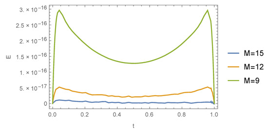
Figure 1. Absolute error E versus t for Example 1 when $k=1,ϵ=0.1$, and $M=\{9,12,15\}$.

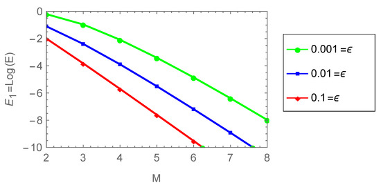
Figure 2. Plot of $E_1=\mathrm{Log}\left(E\right)$ versus M for Example 1 when $k=1$ and $ϵ=\{{10}^{-1},{10}^{-2},{10}^{-3}\}$.

Example 2.

Consider the initial value problem

$$\begin{array}{c}{\displaystyle \frac{d^{2}y}{d{x}^2}}=-30sin\left(30x\right),0\le x\le 10,\hfill \\ y\left(0\right)=0,y^{\prime }\left(0\right)=1,\hfill \end{array}$$

(35)

with analytical solution given by

$$y=\frac{1}{30}sin\left(30x\right).$$

(36)

We use the dilation $x=10t$ to obtain the new initial value problem

$$\begin{array}{c}{\displaystyle \frac{d^{2}y}{d{t}^2}}=-300sin\left(300t\right),0\le t\le 1,\hfill \\ y\left(0\right)=0,y^{\prime }\left(0\right)=1,\hfill \end{array}$$

(37)

with exact solution

$$y=\frac{1}{300}sin\left(300t\right).$$

(38)

Table 3 lists the maximum absolute error E for Example 2 when $k=3$ and $M=\{5,10,15,20\}$.

Table 3. Maximum absolute error E for Example 2 when $k=3$ and $M=\{5,10,15,20\}$.

M	5	10	15	20
E	$2.24\times {10}^{-1}$	$5.28\times {10}^{-3}$	$3.29\times {10}^{-4}$	$5.27\times {10}^{-5}$

Figure 3 illustrates the exact and approximate solutions for different values of M when the value of k is fixed.

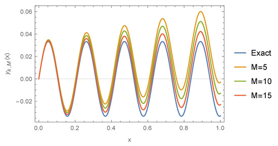
Figure 3. The exact and approximate solutions versus x for Example 2 when $k=3$ and $M=\{5,10,15\}$.

Example 3.

Let us consider the differential equation

$$\begin{array}{c}{\displaystyle \frac{d^{3}y}{d{x}^3}}=xy+(x^3-2x^2-5x-3)e^x,0\le x\le 1,\hfill \\ y\left(0\right)=y\left(1\right)=0,y^{\prime }\left(0\right)=1.\hfill \end{array}$$

(39)

The analytical solution of this initial value problem is given by $y\left(x\right)=x(1-x)e^x$. Table 4 lists the maximum absolute error E of Example 3 when $k=2$ and $M=\{8,10,12,14\}$.

Table 4. Maximum absolute error E for Example 3 when $k=2$ and $M=\{8,10,12,14\}$.

M	8	10	12	14
E	$1.58\times {10}^{-7}$	$2.39\times {10}^{-11}$	$9.38\times {10}^{-14}$	$2.22\times {10}^{-16}$

Figure 4 portraits the exact and approximate solutions for different values of M when the value of k is fixed.

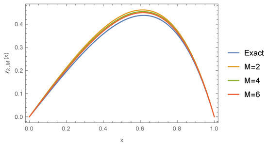
Figure 4. The exact and approximate solutions versus x for Example 3 when $k=2$ and $M=\{2,4,6\}$.

Example 4.

Deformation of an Elastica.The transverse deformation of a thin elastic extensional rod subjected to an axial loading and clamped at its ends is governed by the nonlinear equation [32]

$$\begin{array}{c}\frac{d^{2}y}{d{s}^2}+siny=0,0<s<1,\hfill \\ y\left(0\right)=y\left(1\right)=1.\hfill \end{array}$$

(40)

Due to the nonavailability of the analytical solution of this nonlinear problem, we compare the results for the proposed method with those of the Runge–Kutta sixth-order method (RK6) obtained using Mathematica. Table 5 shows the maximum absolute error E when $s=\{0,0.2,0.4,0.6,0.8,1\}$, $k=1$, and $M=\{4,6,8\}$.

Table 5. Maximum absolute error E for Example 4 when $s=\{0,0.2,0.4,0.6,0.8,1\}$, $k=1$, and $M=\{4,6,8\}$.

s	RK6	$\mathit{M}=4$	$\mathit{M}=6$	$\mathit{M}=8$
0	1	1	1	1
$0.2$	1.0707773	1.0707685	1.0707724	1.070777
$0.4$	1.10651554	1.1065354	1.1065142	1.1065155
$0.6$	1.106542707	1.10654257	1.10654217	1.10654270
$0.8$	1.07084925	1.0708984	1.0708487	1.0708492
1	1	1	1	1

Example 5.

Let us consider the fractional IVP [33]

$$D^{0.5}y\left(t\right)+y\left(t\right)=t^{0.9}+\frac{\Gamma \left(1.9\right)}{\Gamma \left(1.4\right)}{t}^{0.4},y\left(0\right)=0,t\in (0,1),$$

(41)

with the nonsmooth analytical solution $y\left(t\right)=t^{0.9}$. By adopting the transformation $y=u^{0.9},$ Equation (41) is converted into the nonlinear fractional initial value problem

$$D^{0.5}{u}^{0.9}\left(t\right)+u^{0.9}\left(t\right)=t^{0.9}+\frac{\Gamma \left(1.9\right)}{\Gamma \left(1.4\right)}{t}^{0.4},u\left(0\right)=0,t\in (0,1),$$

(42)

with solution $u\left(t\right)=t.$

Let us start with $u\left(t\right)\approx u_1\left(t\right)=\sqrt{\frac{2}{\pi }}{a}_0+\sqrt{\frac{2}{\pi }}{a}_1(2t-1)$ and apply the proposed method for $k=M=1$. We get $c_{1,0}=0.6266570686577501$ and $a_{1,1}=0.5427009409187007$. Therefore, we have

$$u_1\left(t\right)=\sqrt{\frac{2}{\pi }}\left(0.6266570686577501\right)+\sqrt{\frac{2}{\pi }}\left(0.5427009409187007\right)(2t-1)=t+5.55\times {10}^{-17},$$

which is very close to the exact solution.

Table 6 lists the relative error $E_r$ of Example 5 when $k=M=1$.

Table 6. Relative error $E_r$ for Example 5 when $k=M=1$.

t	$0.1$	$0.2$	$0.3$	$0.4$	$0.5$	$0.6$	$0.7$	$0.8$	$0.9$
$E_r$	$4.4094\times {10}^{-16}$	$2.3629\times {10}^{-16}$	$1.6404\times {10}^{-16}$	$1.2662\times {10}^{-16}$	$0.0000$	$0.0000$	$0.0000$	$0.0000$	$0.0000$

Example 6.

Let us consider the fractional oscillator problem [33]

$$D^{\mu }y\left(t\right)+y\left(t\right)=0,y\left(0\right)=1,y^{\prime }\left(0\right)=0,t\in (0,L),$$

(43)

where $1<\mu \le 2$. The analytic solution of Equation (43) is given by

$$y\left(t\right)=\sum _{k=0}^{\infty }\frac{{\left(-t^{\mu }\right)}^k}{\Gamma (k\mu +1)}={\tilde{E}}_{\mu }\left(-t^{\mu }\right),$$

where ${\tilde{E}}_{\mu }\left(t\right)$ is the one-parameter Mittag-Leffler function [33]. For $\mu =2$, the solution reduces to $y\left(t\right)=cos\left(t\right)$. Let us solve Equation (43) when $L=1$ and assume that the approximate solution can be expressed as ${\displaystyle y\left(t\right)\approx y_N\left(t\right)=\sum _{i=0}^N{a}_i{C}_i\left(t\right)}$. We compare the numerical results of the proposed algorithm with those produced by using the truncated series

$$\tilde{y}\left(t\right)=\sum _{k=0}^{10}\frac{{\left(-t^{\mu }\right)}^k}{\Gamma (k\mu +1)},$$

for the case of $k=1,M=16$, and different values of μ.

Table 7 demonstrates that the new method yields good results in the domain $[0,1]$.

Table 7. Maximum absolute error E of Example 6 when $k=1$ and $M=16$.

$\mathit{\mu }$	2	1.95	1.9	1.85	1.8	1.75
E	$3.25\times {10}^{-16}$	$4.71\times {10}^{-14}$	$5.26\times {10}^{-13}$	$7.48\times {10}^{-12}$	$3.25\times {10}^{-11}$	$5.26\times {10}^{-11}$

Example 7.

Let us consider the nonlinear fractional IVP [33,34]

$$D^{\frac{1}{2}}y\left(t\right)+e^{y\left(t\right)}=f\left(t\right),t\in (0,1),$$

(44)

with

$$y\left(0\right)=ln\left(9\right),$$

(45)

where

$${\displaystyle f\left(t\right)=9+t+\frac{2}{\sqrt{\pi (9+t)}}{sinh}^{-1}(\sqrt{t}/3).}$$

The analytic solution of (44) is given by $y\left(t\right)=ln(9+t).$ We apply the proposed algorithm for $k=2$ and $M=\{1,3,5,7,9,11,13\}$. Table 8 lists the maximum absolute error E of problem (44)–(45) versus M.

Table 8. Maximum absolute error E of Example 7 for $k=2$.

M	1	3	5	7	9	11	13
E	$2.36\times {10}^{-1}$	$4.29\times {10}^{-4}$	$8.36\times {10}^{-7}$	$2.37\times {10}^{-10}$	$5.37\times {10}^{-14}$	$4.38\times {10}^{-15}$	$2.43\times {10}^{-16}$

Note. The best absolute maximum errors obtained in [33,34] are E = 2.73 × 10⁻¹⁵ and E = 1.00 × 10⁻¹⁵, respectively, while here we obtained a smaller error with an inferior number of retained modes.

In synthesis, we started by considering a simple boundary value problem in Example 1. Since the technique is not restricted to boundary value problems, we applied the proposed strategy to initial value problems in Examples 2 and 3. To demonstrate the efficiency of the technique on mathematical models, we tackled Example 4, representing the nonlinear deformation of a thin elastic rod. Moreover, fractional-order models were considered in Examples 5–7, which were studied as fractional oscillator problems. It was verified in all cases that the proposed strategy leads to good results.

4. Conclusions

This paper presents a new technique for obtaining the numerical spectral solutions for multi-term fractional-order initial value problems. The derivation of the method is based on the construction of the Chebyshev wavelet operational matrix. One of the advantages of the proposed strategy is its availability both for linear and nonlinear fractional-order initial value problems. A second relevant characteristic of the proposed approach is its high accuracy while adopting a limited number of Chebyshev wavelets. In future work, we will address the applicability of the current technique for stochastic PDEs.

References

- Huang, C.; Zhang, Z.; Song, Q. Spectral Methods for Substantial Fractional Differential Equations. J. Sci. Comput. 2018, 74, 1554–1574. [Google Scholar] [CrossRef]
- Ali, K.K.; Abd El Salam, M.A.; Mohamed, E.M.; Samet, B.; Kumar, S.; Osman, M.S. Numerical solution for generalized nonlinear fractional integro-differential equations with linear functional arguments using Chebyshev series. Adv. Differ. Equ. 2020, 2020, 494. [Google Scholar] [CrossRef]
- Abu Arqub, O. Application of residual power series method for the solution of time-fractional Schrödinger equations in one-dimensional space. Fundam. Inform. 2019, 166, 87–110. [Google Scholar] [CrossRef]
- Abu Arqub, O. Numerical Algorithm for the Solutions of Fractional Order Systems of Dirichlet Function Types with Comparative Analysis. Fundam. Informaticae 2019, 166, 111–137. [Google Scholar] [CrossRef]
- Kajani, M.T.; Vencheh, A.H.; Ghasemi, M. The Chebyshev wavelets operational matrix of integration and product operation matrix. Int. J. Comput. Math. 2009, 86, 1118–1125. [Google Scholar] [CrossRef]
- Ghasemi, M.; Babolian, E.; Kajani, M.T. Numerical solution of linear Fredholm integral equations using sine-cosine wavelets. Int. J. Comput. Math. 2007, 84, 979–987. [Google Scholar] [CrossRef]
- Amaratunga, K.; Williams, J.R.; Qian, S.; Weiss, J. Wavelet-Galerkin solutions for one-dimensional partial differential equations. Int. J. Numer. Methods Eng. 1994, 37, 2703–2716. [Google Scholar] [CrossRef]
- Daubechies, I. Ten Lectures on Wavelets; SIAM: Philadelphia, PA, USA, 1992. [Google Scholar]
- Majak, J.; Pohlak, M.; Eerme, M.; Lepikult, T. Weak formulation based Haar wavelet method for solving differential equations. Appl. Math. Comput. 2009, 211, 488–494. [Google Scholar] [CrossRef]
- Chun, Z.; Zheng, Z. Three-dimensional analysis of functionally graded plate based on the Haar wavelet method. Acta Mech. Solida Sin. 2007, 20, 95–102. [Google Scholar]
- Lam, H.F.; Ng, C.T. A probabilistic method for the detection of obstructed cracks of beam-type structures using spacial wavelet transform. Probabilistic Eng. Mech. 2008, 23, 237–245. [Google Scholar] [CrossRef]
- Noeiaghdam, S.; Sidorov, D.N.; Muftahov, I.R.; Zhukov, A.V. Control of Accuracy on Taylor-Collocation Method for Load Leveling Problem. Bull. Irkutsk. State Univ. Ser. Math. 2019, 30, 59–72. [Google Scholar] [CrossRef]
- Lepik, Ü.; Hein, H. Haar Wavelets; Springer: Berlin/Heidelberg, Germany, 2014. [Google Scholar]
- Abd-Elhameed, W.M.; Doha, E.H.; Youssri, Y.H. New spectral second kind Chebyshev wavelets algorithm for solving linear and nonlinear second-order differential equations involving singular and Bratu type equations. In Abstract and Applied Analysis; Hindawi: London, UK, 2013; Volume 2013. [Google Scholar]
- Robertsson, J.O.A.; Blanch, J.O. Galerkin-Wavelet Modeling of Wave Propagation: Optimal Finite-Difference Stencil Design. Math. Comput. Model. 1994, 19, 31–38. [Google Scholar] [CrossRef]
- Heydari, M.H.; Hooshmandasl, M.R.; Maalek Ghaini, F.M. A new approach of the Chebyshev wavelets method for partial differential equations with boundary conditions of the telegraph type. Appl. Math. Model. 2014, 38, 1597–1606. [Google Scholar] [CrossRef]
- Kumar, V.; Mehra, M. Wavelet optimized finite difference method using interpolating wavelets for self-adjoint singularly perturbed problems. J. Comput. Appl. Math. 2009, 230, 803–812. [Google Scholar] [CrossRef]
- Turgut, A.K.; Triki, H.; Dhawan, S.; Moshokoa, S.K.; Ullah, M.Z.; Biswas, A. Computational Analysis of Shallow Water Waves with Korteweg-de Vries Equation. Sci. Iran. 2018, 25, 2582–2597. [Google Scholar]
- Turgut, A.K.; Dhawan, S. A practical and powerful approach to potential KdV and Benjamin equations. Beni-Suef Univ. J. Basic Appl. Sci. 2017, 6, 383–390. [Google Scholar]
- Turgut, A.K.; Dhawan, S.; Karakoc, S.B.G.; Raslan, K.R. Numerical Study of Rosenau-KdV Equation Using Finite Element Method Based on Collocation Approach. Math. Model. Anal. 2017, 22, 373–388. [Google Scholar]
- Machado, J.T.; Costa, A.C.; Quelhas, M.D. Wavelet analysis of human DNA. Genomics 2011, 98, 155–163. [Google Scholar] [CrossRef] [PubMed]
- Mao, Z.; Em Karniadakis, G. A Spectral Method (of Exponential Convergence) for Singular Solutions of the Diffusion Equation with General Two-Sided Fractional Derivative. SIAM J. Numer. Anal. 2018, 56, 24–49. [Google Scholar] [CrossRef]
- Kumar, S.; Kumar, R.; Osman, M.S.; Samet, B. A wavelet based numerical scheme for fractional order SEIR epidemic of measles by using Genocchi polynomials. Numer. Methods Partial. Equations 2021, 37, 1250–1268. [Google Scholar] [CrossRef]
- Yarmohammadi, M.; Javadi, S.; Babolian, E. Spectral iterative method and convergence analysis for solving nonlinear fractional differential equation. J. Comput. Phys. 2018, 359, 436–450. [Google Scholar] [CrossRef]
- Mason, J.C.; Handscomb, D.C. Chebyshev Polynomials; CRC Press: Boca Raton, FL, USA, 2002. [Google Scholar]
- Sweilam, N.H.; Nagy, A.M.; El-Sayed, A.A. Second kind shifted Chebyshev polynomials for solving space fractional order diffusion equation. Chaos Solitons Fractals 2015, 73, 141–147. [Google Scholar] [CrossRef]
- Piessens, R. Computing integral transforms and solving integral equations using Chebyshev polynomial approximations. J. Comput. Appl. Math. 2000, 121, 113–124. [Google Scholar] [CrossRef]
- Babolian, E.; Fattahzadeh, F. Numerical solution of differential equations by using Chebyshev wavelet operational matrix of integration. Appl. Math. Comput. 2007, 188, 417–426. [Google Scholar] [CrossRef]
- Zhou, F.; Xu, X. Numerical solution of the convection diffusion equations by the second kind Chebyshev wavelets. Appl. Math. Comput. 2014, 247, 353–367. [Google Scholar] [CrossRef]
- Mohammadi, F.; Hosseini, M.M. A comparative study of numerical methods for solving quadratic Riccati differential equations. J. Franklin Inst. 2011, 348, 156–164. [Google Scholar] [CrossRef]
- Yuanlu, L.I. Solving a nonlinear fractional differential equation using Chebyshev wavelets. Commun. Nonlinear Sci. Numer. 2010, 15, 2284–2292. [Google Scholar]
- Singh, I.; Arun, P.; Lima, F. Fourier analysis of nonlinear pendulum oscillations. Rev. Bras. Ensino Fis. 2018, 40, e1305. [Google Scholar] [CrossRef]
- Abd-Elhameed, W.M.; Youssri, Y.H. Fifth-kind orthonormal Chebyshev polynomial solutions for fractional differential equations. Comput. Appl. Math. 2018, 37, 2897–2921. [Google Scholar] [CrossRef]
- Atta, A.G.; Moatimid, G.M.; Youssri, Y.H. Generalized Fibonaacci operational collocation approach for fractional initial value problem. Int. J. Appl. Comput. Math. 2018, 5, 9. [Google Scholar] [CrossRef]
Publisher’s Note: MDPI stays neutral with regard to jurisdictional claims in published maps and institutional affiliations. |
© 2021 by the authors. Licensee MDPI, Basel, Switzerland. This article is an open access article distributed under the terms and conditions of the Creative Commons Attribution (CC BY) license (http://creativecommons.org/licenses/by/4.0/).