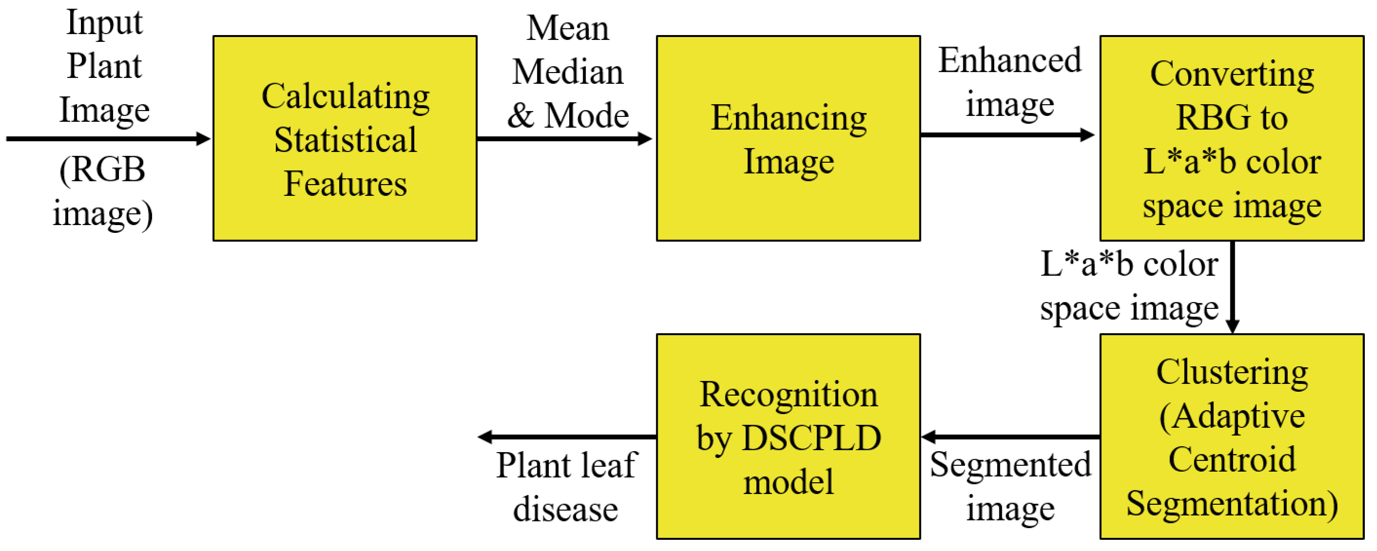
Article

Plant Leaf Disease Recognition Using Depth-Wise Separable Convolution-Based Models

by
Syed Mohammad Minhaz Hossain
1,2,
Kaushik Deb
1,*,
Pranab Kumar Dhar
1 and
Takeshi Koshiba
3
1
Department of Computer Science & Engineering, Chittagong University of Engineering & Technology (CUET), Chattogram 4349, Bangladesh
2
Department of Computer Science & Engineering, Premier University, Chattogram 4000, Bangladesh
3
Faculty of Education and Integrated Arts and Sciences, Waseda University, 1-6-1 Nishiwaseda, Shinjuku-ku, Tokyo 169-8050, Japan
*
Author to whom correspondence should be addressed.
Symmetry 2021, 13(3), 511; https://doi.org/10.3390/sym13030511
Submission received: 3 March 2021 / Revised: 13 March 2021 / Accepted: 18 March 2021 / Published: 21 March 2021

Abstract

:
Proper plant leaf disease (PLD) detection is challenging in complex backgrounds and under different capture conditions. For this reason, initially, modified adaptive centroid-based segmentation (ACS) is used to trace the proper region of interest (ROI). Automatic initialization of the number of clusters (K) using modified ACS before recognition increases tracing ROI’s scalability even for symmetrical features in various plants. Besides, convolutional neural network (CNN)-based PLD recognition models achieve adequate accuracy to some extent. However, memory requirements (large-scaled parameters) and the high computational cost of CNN-based PLD models are burning issues for the memory restricted mobile and IoT-based devices. Therefore, after tracing ROIs, three proposed depth-wise separable convolutional PLD (DSCPLD) models, such as segmented modified DSCPLD (S-modified MobileNet), segmented reduced DSCPLD (S-reduced MobileNet), and segmented extended DSCPLD (S-extended MobileNet), are utilized to represent the constructive trade-off among accuracy, model size, and computational latency. Moreover, we have compared our proposed DSCPLD recognition models with state-of-the-art models, such as MobileNet, VGG16, VGG19, and AlexNet. Among segmented-based DSCPLD models, S-modified MobileNet achieves the best accuracy of 99.55% and F1-sore of 97.07%. Besides, we have simulated our DSCPLD models using both full plant leaf images and segmented plant leaf images and conclude that, after using modified ACS, all models increase their accuracy and F1-score. Furthermore, a new plant leaf dataset containing 6580 images of eight plants was used to experiment with several depth-wise separable convolution models.

1. Introduction

Plant disease is one of the crucial reasons for food insecurity all over the world. It reduces the quantity of plant production and the quality of plants [1]. For this reason, early detection and protective measures of various plant diseases are a significant part of plant monitoring in the agro-industry. However, early detection of plant disorders and their categories are somehow tough with the naked eye and susceptible to human error. Supports of machine learning and computer vision opens the opportunities of automatic image-based decision [2], monitoring, 3D reconstruction [3], and robot-guidance in an agricultural field.
Plant diseases can be detected through leaves, roots, stems, and other parts of fruits and vegetables. For early detection of plant diseases, it is essential to detect the symptoms from the plant part. This monitoring is vital in plant diagnosis. Sometimes, symptoms appeared on specific parts of plants. Sometimes, symptoms are grown in one plant part and then speared over the other plant part. In this phenomenon, there is a chance of diminishing symptoms in the later stage of plant diseases. Therefore, choosing the right plant part is a significantly important. However, in our depth-wise separable convolutional plant leaf disease (DSCPLD) recognition framework, we consider the detection of plant diseases which spreads through young leaves.
Conventional machine learning algorithms are only appropriate and effective in specific circumstances and setup [4]. Under diversification and uncontrolled conditions, accuracy of these algorithms fall drastically. With the breakthrough of deep learning [5], researchers encouraged to apply deep learning to get state-of-the-art performance in agriculture. There are still some challenges in this perspective, such as memory restriction of devices (number of parameters), sustainable accuracy (not a fall in testing a new dataset), and computational latency (floating point operations and multiply accumulate operation).
Sustainable accuracy is a challenge in convolutional neural network (CNN)-based plant leaf disease (PLD) recognition models due to a fall in accuracy after adding new PLD images in References [6,7]. To overcome this challenge, it is essential to eradicate the unnecessary information from PLD images, and consider the heterogeneous image backgrounds. Moreover, some works are limited to symmetric backgrounds [6,7,8,9,10] and sensitive to image capturing conditions [11].
Moreover, most of the state-of-the-art CNN models, such as LeNet [12] in Reference [13], VGG in References [6,10,14], GoogleNet [15] in Reference [7], ResNet50, ResNet101, ResNet152, InceptionV4 in Reference [10], ResNet34 in Reference [16], Student-teacher CNN in Reference [9], AlexNet [17] in References [6,7,18,19], DenseNet in Reference [10], InceptionV3, DenseNet201, and ResNet in Reference [19], and custom CNN model in References [20,21,22], achieve better accuracy for their deep and dense structures. Faster R-CNN, faster R-CNN with FPN, faster R-CNN with TDM, YOLOV3, SSD513, and RetinaNet are used in Reference [19] for detecting disease symptoms in plants. However still, these models have restriction to memory (space) for mobile and IoT device-based PLD recognition and computational costs for faster convergence.
To overcome the above-mentioned limitations of existing PLD recognition frameworks, we propose depth-wise separable convolution (DSC)-based PLD (DSCPLD) recognition framework. In these frameworks, we introduce a segmentation technique called adaptive centroid-based segmentation (ACS) that traces the proper regions of interest (ROIs) under different circumstances, such as images with shading, images behind objects, and shrunk images overlapped with other plant leaves, in Reference [23]. Automatic initialization of optimal cluster number (K) from the PLD images in our modified ACS solves the insensitivity to proper K in Reference [20]. This technique helps the DSCPLD recognition model avoid noises and destruction in ROIs irrespective of real field environments. This phenomenon increases the generalization ability of DSCPLD and restricts to fall in accuracy depicted in References [6,7].
Moreover, to reduce the parameters and computational cost for mobile and IoT handled applications, depth-wise separable convolutional (DSC)-based PLD (DSCPLD) models are developed based on MobileNet [24,25]. Finally, a comprehensive trade-off is drawn among accuracy, parameter size, and computation latency for mobile and IoT-based PLD recognition.
The primary contributions of this paper:
(i)
a new dataset is introduced, including the diversified backgrounds of PLD images. PLD images are investigated under both direction and illumination-based augmentations to recognize the PLDs in natural circumstances.
(ii)
introduce a modified segmentation technique that can trace the accurate ROI irrespective of diversified backgrounds, under uneven illuminations and orientations. This phenomenon increases the sustainability of our DSCPLD recognition framework. Moreover, it also decreases the possibility of a fall in accuracy for testing an independent dataset.
(iii)
various modified and reduced DSC-based architectures are developed using segmented images and full PLD images to establish a concrete trade-off among accuracy, parameter size, and computation latency for mobile and IoT-based PLD recognition.
The rest of the paper is organized as follows. Section 2 discusses the related works; proposed model for recognizing plant leaf diseases is presented in Section 3; experimental results and observations are illustrated in Section 4; and, finally, the paper is concluded in Section 5.

2. Literature Review

Manual plant disease identification and monitoring the plant health is a hectic, industrious, and prolonged task. More often, it is subjective, lavish, and challenging. Therefore, researchers investigate automatic detection and identification techniques to solve this problem and make the farmers’ activities more efficient and accurate.
Conventional machine learning algorithms are only appropriate and effective in specific circumstances and setup [4]. Under diversification and uncontrolled conditions, the accuracy of these algorithms falls drastically. With the breakthrough of deep learning [5], researchers encouraged to apply deep learning to get state-of-the-art performance in agriculture.
Numerous modifications are done in CNN architectures for recognizing PLDs in recent years. Ferentinos et al. [6] performed CNN models for detecting 58 diseases of 25 plants and achieved 99.53% success rates for VGG. However, accuracy was reduced for previously unknown data to the training model and fell by 25–35%. In Reference [7], 26 PLDS of 14 crop species were identified using GoogleNet and AlexNet by transfer learning and learning from image scratch and achieved an accuracy of 99.35%. However, this work has limitations, such as images are taken under control, and accuracy falls drastically (above 31%) for the independent test dataset. Sladojevic et al. [8] performed Modified CaffeNet using ImageNet on more than 3000 images of 13 classes collected from Internet resources and achieved an accuracy of 96.3%. However, this work still has a limitation of a small number of sample images in the dataset and can be improved by increasing the samples. In Reference [10], for detecting 38 PLDs of 14 plants, VGG, ResNet, Inception and DenseNet were performed and achieved 99.75% accuracy for DenseNet. However, still, the computational cost is a fact. Another limitation is considering homogeneous backgrounds with a single leaf. Liang et al. [11] proposed a custom CNN model to perform on rice blast disease recognition and achieved better accuracy than using feature extraction technique, such as histogram-based local binary pattern (HLBP) and haar wavelet transformation (HaarWT). In this work, custom CNN architecture achieved the best accuracy of 95.83%. However, this work is sensitive to image capturing conditions and needs to expand the number of samples.
In Reference [13], two common diseases of banana were detected using LeNet architecture. The experiment is performed on 3700 banana color images collected from PlantVillage and also executed in grayscale images. In this work, LeNet architecture achieved 92–99% accuracy. However, their proposed work still has limitations in taking the image in real conditions, and accuracy falls significantly in grayscale images. Rahman et al. [14], performed two state-of-the-art CNN architectures, such as VGG16 and InceptionV3, for recognizing rice diseases. Besides, they have proposed a two-stage CNN model, which is effective for memory restricted devices. The authors identified that their manual process of dividing symptom classes might cause misclassifications. Liu et al. proposed PLD recognition models, including five CNN architectures (AlexNet, GoogleNet, ResNet20, and VGGNet16) and two machine learning algorithms, such as support vector machine (SVM) and backpropagation neural network (BPNN), for recognizing apple leaves, in Reference [18]. Among them, modified AlexNet achieved the best accuracy of 97.62%. As future work, they figured out the need to expand the dataset. Arsenovic et al. performed various state-of-the-art CNN architectures AlexNet, VGG19, InceptionV3, DenseNet201, and ResNet with generative adversarial network (GAN) data augmentation for recognizing 42 classes of 12 species in Reference [19] and achieved the best accuracy of 90.88%. Besides, in this work, faster R-CNN, faster R-CNN with FPN, faster R-CNN with TDM, YOLOV3, SSD513, and RetinaNet were performed for object detection in the plant. Moreover, this work proves the generalization by executing independent training and test dataset. They pointed out that in future, they will integrate their work into a mobile application. However, there is no analysis of computational complexity and memory requirements for mobile devices in this work. Authors in Reference [20] trained the custom CNN models for both full images and segmented images of 10 diseases and achieved 98.6% for S-CNN and 42.3% for F-CNN and having limitations of proper segmentation in uneven illuminations and different orientations.
Chen et al. [21] proposed a custom CNN model named LeafNet for extracting features of diseases for tea leaf images. Moreover, in this work, dense scale-invariant feature transform features (DFTF) were also extracted and later used to construct a bag of visual words (BOVW) model. However, then support vector machine (SVM), and multi-layer perceptron (MLP) classifiers were performed to classify diseases. Among all the models, LeafNet algorithm identified tea leaf diseases with an accuracy of 90.16%. Authors figured out to investigate their model’s universality for different species. Transfer learning was used in Reference [26] to identify plants. Six state-of-the-art architectures (AlexNet, DenseNet169, InceptionV3, ResNet34, SqueezeNet-1.1, and VGG13) were performed on PlantVillage dataset and achieved an accuracy of more than 99.2%. A saliency map as a visualization method helped to learn the diversified features. In Reference [27], the authors investigated the computational complexity and memory requirements for plant leaf disease recognition. In Reference [28], authors performed faster R-CNN, region-based fully convolutional network (R-FCN) and SSD, backend with VGG16 to recognize the tomato diseases. Their motivations are to overcome limitations of tracing disease features in different illumination and complex background. They used 5000 images and later increased the images using geometrical and intensity transformations. Despite data augmentation, obtained accuracy is not high and on an average 85.98%. In Reference [29], the authors proved the impact of segmentation and background removal. To do so, the authors used 1567 images to identify multiple diseases in the same sample. Pre-trained GoogLeNet CNN architecture achieved 75 to 100% accuracy depending on species. The work in Reference [30] represented a concrete study among various pooling strategies, such as mean-pooling, max-pooling, and stochastic pooling, to recognize rice leaf diseases using CNNs. In this work, CNN achieved 95.48% for stochastic pooling. The authors pointed out the need to expand the sample images and to optimize the number of parameters. In Reference [31], machine learning-based algorithms support vector machine (SVM), linear regression (LR), and random forest (RF) are performed to classify six classes of peanut leaf diseases. Moreover, five CNN models: VGG, AlexNet, ResNet50, DenseNet121, and InceptionV3 are investigated with augmentation and without augmentation. From them, with augmentation DenseNet121 achieved 95.98% and without augmentation ResNet50 achieved 94.36%. The authors investigated that with augmentation and ensemble with machine learning algorithms, deep learning models achieved better accuracy. Ensemble of DenseNet121 and RF achieved better accuracy of 97.59%. However, this work still has limitations of less number of disease images and classes.
In recent times, some comprehensive surveys [4,23,27] are conducted to sum up the limitations of current PLD recognition methods. Some challenges of current PLD recognition works are as follows:
(i)
diversified data with heterogeneous backgrounds, such as natural, complex, and under uncontrolled capture conditions.
(ii)
more accurate identification due to similar symptoms in various plant diseases.
(iii)
drastically fall in accuracy.
(iv)
disease phases identification due to symptom changes.
Most of the cases, authors solved the above mentioned problems to a certain extent; however, there are many opportunities to improve the PLD recognition models.
(i)
sustainable accuracy. To do so:
  • use diversified data with heterogeneous backgrounds, such as natural, complex backgrounds, and under uncontrolled capture conditions.
  • use segmentation phase to eradicate unnecessary noises.
  • test on a dataset that is not part of a train set.
(ii)
investigates memory requirements and computational latency to integrate our model into mobile.
Table 1 represents the brief descriptions of various PLD recognition frameworks, and Table 2 represents the limitations of existing PLD recognition frameworks.

3. Materials and Proposed Method

In this section, our proposed framework is discussed in detail. Initially, the disease recognition framework optionally enhances the RGB PLD image, and then ACS is applied to trace the ROIs. Finally, our DSC-based architectures based on the modification of MobileNet [24,25] is performed to recognize the PLDs. The proposed DSCPLD recognition framework has been exhibited in Figure 1.

3.1. Dataset

In the experiment, 4606 original RGB images of eight different plants are used to train, and 1316 PLD images are used to validate. These images are collected from the PlantVillage dataset [32], except the images for rice disease. Rice disease images are gathered from the Rice disease image dataset [33] in Kaggle, the International Rice Research Institute (IRRI) [34], and Bangladesh Rice Research Institute (BRRI) [35]. We vary the natural (in Figure 2a,b,k), plain (in Figure 2e–j,l), and complex (in Figure 2a,f,g) image backgrounds to trace a disease properly in different backgrounds. Further, the framework considers various symptoms, such as small (in Figure 2d,f,h,j,l), large (in Figure 2e,g), isolated (in Figure 2d–h,j,l), and spread (in Figure 2a–c,e,g,i,k). Twelve disease samples of eight plants are represented, as shown in Figure 2. For generalization, 658 independent images from twelve different classes are used during the test phase. Complete information regarding the PLD dataset is described in Table 3.

3.1.1. Adding Direction Disturbance to Dataset

One of the challenges in PLD recognition is uncontrolled capturing conditions, such as image capturing in different orientations. Due to the relative position of the acquisition device, the characteristics of images can be spatially transformed. However, it is challenging to have PLD images from every angle to meet the challenges. For this reason, we use different directional augmentation to expand our PLD dataset. This augmentation increases the adaptability of our DSCPLD models.
Rotation in an image refers to rotation of all pixels in a certain angle. Suppose P(x0,y0) is a certain pixel in an image. After rotating by θ° clockwise, this pixel changes into position P(x,y). The co-ordinates of P(x0,y0) and P(x,y) are represented in Equations (1) and (2).
x 0 = r c o s α y 0 = r s i n α ,
x = r c o s ( α θ ) y = r s i n ( α θ ) .
The mirror symmetry in an image refers to expand all pixels after selecting a line as an axis. In horizontal mirror symmetry, selects a vertical line in an image and expands all pixels. However, in vertical mirror symmetry, selects a horizontal line in an image and expand all pixels. Suppose an image’s width is w, P(x0,y0) is a certain pixel in an image. The point’s coordinate will be as shown in Equations (3) and (4), respectively, after applying horizontal and vertical mirror symmetry.
x 0 = w x 0 y 0 = y 0 ,
x = x 0 y = w y 0 .
In our DSCPLD recognition framework, we use rotation and mirror symmetry (vertical and horizontal) on our original PLD images as shown in Figure 3a–g.

3.1.2. Adding Lighting Disturbance to Dataset

Weather condition is one of the challenges in capturing images. Sunlight orientation, shadow and foggy weather have an impact on the brightness of acquired images. For improving the generalization ability, we generate images by adjusting the sharpness value, brightness value, and contrast value.
Sharpening the image means to enhance edges and borders as the objects in that image emerge. Suppose, a pixel in RGB is P(x,y) and P ( x , y ) = [ R ( x , y ) , B ( x , y ) , G ( x , y ) ] T . For adding sharpness to the image, we apply Laplace to that pixel using Equation (5).
2 [ P ( x , y ) ] = 2 [ R ( x , y ) ] 2 [ G ( x , y ) ] 2 [ B ( x , y ) ] .
Brightness in an image refers to the increase or decrease of RGB values of a pixel. Suppose B 0 is the original RGB value and d is the brightness transformation factors. After applying the brightness transformation factor, we get the adjusted RGB value (B) as shown in Equation (6).
B = B 0 × ( 1 + d ) .
In contrast, in an image, a larger RGB value is increased, and a smaller RGB value is decreased based on the brightness’s median. Suppose B 0 is the original RGB value, d is the brightness transformation factors, and i is the brightness’s median. After applying the contrast, we get the adjusted RGB value (B) as shown in Equation (7).
B = i + ( B 0 i ) × ( 1 + d ) .
We apply various illumination-based augmentations in our DSCPLD recognition framework, such as changes in contrast, brightness, and sharpness, on our PLD dataset, as shown in Figure 4a–g.

3.2. Enhancing Image Using Statistical Features

To improve the PLD image quality, the enhancement is optional as it depends on the magnitude of degradation. Two enhancement conditions have been used here using statistical features, such as mean ( μ ), median ( x ), and mode ( M 0 ) of a plant leaf image. The two conditions for image enhancement are devised as in Equations (8) and (9).
μ < x < M 0 ,
μ < x > M 0 .
The performance of image enhancement conditions is as shown in Figure 5a–h. For having symmetric color in ROI and image background, our enhancement condition performs well, as shown in Figure 5a, using Equation (8). Using Equation (9), for presence of leaf shadow on the image background, our enhancement condition performs well as shown in Figure 5b.

3.3. Clustering by Adaptive Centroid-Based Segmentation

The modified adaptive centroid-based segmentation (ACS) has been applied once the PLD image quality has been enhanced. Initially, RGB PLD image is converted to L*a*b color space PLD image. Our modified ACS focuses on initializing optimal K, automatically from the leaf image based on chromatic value (a and b), to eliminate the limitation of lacking sensitivity of K in Reference [20]. In traditional K-means clustering, Euclidean distance between each point and centroid has been calculated to check whether the point is in the same cluster. In the modified ACS, data points are investigated for eligibility by using a statistical threshold. After that, we calculate the distance between these eligible points and centroids, thus, comparatively reducing the effort to form clusters and restrict the misclustering of data points. The statistical threshold (ST) value has been calculated by Equation (10).
S T = i = 1 N ( ( X i C ) 2 ) / N .
where X i , C, and N stand for data points, the centroid of data points, and the total number of data points. The automatic initialization of K using ACS can effectively detect image characteristics for different orientations and illuminations. ACS also increases the scalability of the proposed segmentation technique, as shown in Figure 5f,h over traditional segmentation technique, as shown in Figure 5e,g. A few examples under different circumstances are as shown in Figure 6a–e. Rice leaf image in natural background with presence of shadow and shrunk is as shown in Figure 6a. A blur rice leaf image in natural background with same color light is presented in Figure 6b. In Figure 6c, there is a rice leaf image with symmetric color of ROI and shadow of objects behind it. Figure 6d represents a rice leaf image with complex background. A potato image with the presence of the shadow behind the ROIs, as shown in Figure 6e. Segmented results of plant samples in Figure 6a–e are presented, respectively, in Figure 6f–j.

3.4. Recognition by DSCPLD Models

In this section, we describe the basic operations of depth-wise separable convolution, basic modules of MobileNet variations, DSCPLD model design, and tuning.

3.4.1. Depth-wise Separable Convolution

Our PLD recognition framework is constru cted based on depth-wise separable convolution (DSC). Depth-wise separable convolution comprises two convolutions; one is depth-wise convolution, and another one is point-wise convolution. DSC splits 3 × 3 convolutions into a 3 × 3 depth-wise convolution and a 1 × 1 point-wise convolution. Traditional convolution acts both the channel-wise and spatial-wise computation in a particular step. In traditional convolution, convolution for each input channel is done with one specific kernel, and the convolved output is the convolved results from all the channels. On the contrary, DSC breaks the operation into two steps: Depth-wise convolution is a channel-wise convolution that performs the convolution using individual input channels. Then, do point-wise convolution, which is similar to traditional convolution with kernel size 1 × 1. Point-wise convolution combines the results of each channel. The comparison among the convolutions is as shown in Figure 7. The computational cost of the traditional convolution ( C o s t C ) is shown in Equation (11).
C o s t C = M . K . K . N . P .
However, in case of depth-wise separable convolution, the computational cost ( C o s t D ) is shown in Equation (12).
C o s t D = M . M . K . K . N + M . M . N . P .
The weight ( W C ) considered for traditional convolution is shown in Equation (13).
W C = K . K . N . P .
The weight ( W D ) considered for depth-wise separable convolution is shown in Equation (14).
W D = K . K . N + N . P ,
where N is the number of input channel, and P is the number of output channel. K × K is the width and height of the kernel, and M × M is the width and height of an input feature map. Finally, the reduction on weights ( F W ) and operation ( F Cos t ) are derived in Equations (15) and (16).
F w = W D W C = 1 P + 1 K 2 .
F Cost = C o s t D C o s t C = 1 P + 1 K 2 .
Using 3 × 3 depth-wise separable convolution [24], the computation cost decreases 8 or 9 times than the traditional convolutional layer.

3.4.2. Basic Depth-wise Separable Convolution Modules

Numerous CNN models are constructed based on the modifications of convolution layers. AlexNet, VGG, Inception, ResNet are performed comparatively better in recognizing PLD. However, it is not feasible to consider those models for mobile and IoT-based PLD recognition applications due to their large number of network parameters. For getting the better of it, depth-wise separable convolutions are proposed to expand the trade-off effectiveness among accuracy, parameter size, and computational latency. There are two variations in depth-wise separable convolution: point-wise convolution adjacent to depth-wise convolution, as shown in Figure 8b, and batch normalization and ReLU used between each of depth-wise convolution and point-wise convolution, as shown in Figure 8c. From these concepts, we propose three architectures; one is based on Figure 8b, depicted in Reference [25], called modified MobileNet (called S-modified MobileNet for segmented images and F-modified MobileNet for full leaf images). The other two are reduced MobileNet (called S-reduced MobileNet for segmented images and F-reduced MobileNet for full leaf images) based on MobileNet version in Reference [24], as shown in Figure 8c, and another one is extended MobileNet (called S-extended MobileNet for segmented images and F-extended MobileNet for full leaf images) based on Figure 8c using max-pooling layer once after last point-wise convolution.
In MobileNetV2 [36], linear bottleneck and inverted residual structure are added to build an efficient structures. It includes an additional 1 × 1 convolution followed by pair of depth-wise convolution and point-wise convolution. Moreover, there is a residual connection between input and output depending on their same number of channels as shown in Figure 9.
In MobileNetV3 [37], with all these layers modified swish non-linearities, and squeeze and excitation are added to make the MobileNet efficient.
There are two extra hyper-parameters in MobileNet versions: width multiplier ( α ) and resolution multiplier ( ρ ). Width multiplier ( α ) is used to make the network thinner and resolution multiplier ( ρ ) is used to control the input and size of each layer.

3.4.3. Model Design and Tuning

As one of our goals was to establish a concrete representation of trade-off among the accuracy, parameter size and computational latency, we compared our DSCPLD recognition models with state-of-the-art CNN models, such as AlexNet (input size: 224 × 224), VGG (input size: 180 × 180), MobileNetV1 (input size: 224 × 224), MobileNetV2 (input size: 224 × 224), and MobileNetV3 (input size: 224 × 224). Architectures of three DSCPLD recognition models based on MobileNet are represented in Table 4 with input size 224 × 224, Table 5 with input size 224 × 224 and Table 6 with input size 256 × 256, respectively. We split our PLD dataset into three parts: train, validation, and test in the ratio of 70-20-10, as shown in Table 3. In the training phase, we train our DSCPLD models and other state-of-the-art models using our PLD dataset. We validate our DSCPLD models using PLD images from our dataset for tuning hyper-parameters and alleviating the biasness of those models. For generalization, we test our DSCPLD models with our PLD dataset and another benchmark rice dataset. Performance of models is evaluated on mean test accuracy (mAcc) and mean F1-score (mF). Then, we investigate the impact of segmentation by executing all the models using both segmented and full leaf images. For all the experiments, various optimizers, such as Adam, SGD, and RMSprop, are used to optimize weights and minimizes the loss. We investigate the best loss of our DSCPLD models using learning rate of 0.001 and 0.0001. Momentum for SGD optimizers is 0.8 and 0.9. We use categorical cross-entropy as loss function and softmax as activation in output layers for multi-class PLD recognition. Hyper-parameters used to tune the models for recognizing PLDs are shown in Table 7.

4. Experimental Result and Observation

4.1. Hardware Requirements

All the experiments were conducted on a configuration of AMD Ryzen 7 2700X Eight-core 3.7 GHz Processor. The operating system is Ubuntu version 20.04, 32 GB RAM, Nvidia GeForce RTX 2060 Super of 8 GB GPU Memory. Keras backend with TensorFlow was used.

4.2. Dataset Collection

In this experiment, 4606 images of eight plants of size 256 × 256 pixels are used to train, and 1316 PLD images are used to validate. Moreover, independent of 658 PLD images are used to test twelve classes. Data are collected from different internet sources and benchmark dataset. Source-wise statistics of our PLD image dataset are shown in Table 8.

4.3. Performance Evaluation of Our DSCPLD Frameworks Based on Mean Accuracy and Mean F1-Score Using Segmented Images

To evaluate our proposed DSCPLD recognition model’s performance, we compare them with MobileNetV1, MobileNetV2, MobileNetV3, VGG16, VGG19, and AlexNet based on train, validation, test accuracy, and F1-score. To do so, we first segment the images using our modified ACS and then apply the images to the models. In our evaluation, as the number of samples is imbalanced classwise, we use some performance indicators, such as mean class accuracy (mAcc) and mean class F1-score (mF), as Equations (17)–(23).
Mean Class Accuracy of a model ( mCAcc ) = k ( Recognition rate of each class × N k ) N ,
Recognition rate of a class = True Positive + True Negative Number of all samples of that class ,
Mean Class Precision of a model ( mCP ) = k ( Precision of each class × N k ) N ,
Precision of a class = True Positive True Positive + False Positive ,
Mean Class Recall of a model ( mCR ) = k ( Recall of each class × N k ) N ,
Recall of a class = True Positive True Positive + False Negative ,
Mean F 1 score of a class ( mF ) = 2 × mP × mR mP + mR ,
where k represents each of the class, N k indicates the number of samples in class k, and N is the total number of samples used to test the model.
The comparison among PLD recognition models using segmented images with perspective to accuracies and mean F1-score (mF) is as shown in Table 9.

4.4. Performance Evaluation of Our DSCPLD Frameworks Using Segmented Images Based on Model Size and Computational Latency

We calculate the number of training parameters for memory requirements and floating-point operation (FLOPs) and multiply-accumulate operation (MACC) for computational latency for further evaluation. FLOPs are used to measure the complexity of a model and represent the operation of a model. MACC represents the number of additions and multiplications (dot product computation). Calculations of FLOPs and MACC are performed, as shown in Reference [38]. Concrete memory requirements and computational complexity representation of various models are as shown in Table 10.

4.5. Selection of the Best DSCPLD Framework Based on All Criteria

From Table 9, it is shown that S-modified MobileNet and state-of-the-art architecture MobileNetV3 achieve the best mean test accuracy of 99.55% on our PLD dataset. However, MobileNetV3 requires almost 5–10 times parameters than our proposed three DSCPLD recognition models, as shown in Table 10. Besides, S-modified MobileNet achieves the best mean F1-score of 97.07%. According to model size, FLOPs and MACCs as shown in Table 10, the best one is S-reduced MobileNet; however, considering all factors included in Table 9 and Table 10, S-modified MobileNet is best among all the PLD recognition models for mobile and IoT-based PLD recognition.
Confusion metrices, ROC curves, Accuracy, and Loss curves of our three proposed DSCPLD models are as shown in Figure 10a–d, Figure 11a–d, and Figure 12a–d.

4.6. Processing Steps Using Our DSCPLD Framework

A processing example of rice blast leaf image using S-modified MobileNet is shown in Figure 13a–r with some activation on each of the layers. The presence of symmetrical color in both infected area and image background makes this leaf disease recognition quite difficult. Results in Figure 13a–r proves the followings:
  • effectiveness of our segmentation technique in a complex situation.
  • accurate recognition in natural background.

4.7. Performance Evaluation of Our PLD Frameworks Using Segmented Images and Full Leaf Images

Further, we execute DSCPLD models (F-modified MobileNet, F-reduced MobileNet and F-extended MobileNet) and six state-of-the-art CNN models (VGG16, VGG19, AlexNet, MobileNetV1, MobileNetV2, and MobileNetV2) using full leaf images to evaluate the effectiveness of segmentation. The performance of DSCPLD models is shown in Table 11. From Table 11, F-modified MobileNet (modified mobileNet using full leaf images) achieves the highest accuracy of 99.10%. The performance comparisons among the segmented-based DSCPLD models and DSCPLD models using full leaf images are as shown in Table 12, Table 13 and Table 14. The confusion matrix and ROC curve of F-modified MobileNet are shown in Figure 14a,b.

4.8. Performance Evaluation of Our PLD Frameworks Using Various Parameters on MobileNetV3

Further, we execute MobileNetV3 on segmented PLD images and investigate the results using width multipliers 0.25, 0.5, 0.75, and 1.0 with fixed size of image 224 × 224 as shown in Table 15. Then, we execute resolutions 128, 160, 192, and 224 with a definite width multiplier 1.0 as shown in Table 16. From Table 15 and Table 16, it is observed that S-modified MobileNet is more effective than the variations experimented on MobileNetV3 based on accuracy, computational latency, and model size.
From Table 12, it is shown that S-modified MobileNet achieves improved accuracy of 0.45% and F1-score of 0.44% more than the F-modified MobileNet due to eradication of extra noises from the leaf images in situations, such that obstacles behind the leaf images, images with shading and shrunk images overlapped with other plant leaves, as shown in Figure 6a–e.

4.9. Evaluation of Generalization for Our DSCPLD Framework

As in the segmentation phase, noises are removed, only ROI with symptoms is applied to our DSCPLD recognition models. This phenomenon increases the generalization and sustainability of those PLD recognition models. For evaluation of generalization in our S-modified MobiNet, we test this model using a rice leaf disease dataset (https://github.com/aldrin233/RiceDiseases-DataSet (accessed on 17 February 2021)). We consider only rice blast and rice bacterial blight leaf images for testing our DSCPLD model. There are 160 infected rice blast leaf images, including 80 rotated rice blast leaf disease images and 180 rice bacterial leaf blight images, including 90 rotated images. S-modified MobileNet achieves the best mean test accuracy of 98.53% for recognizing the two rice disease classes, and accuracy (mAcc) falls down 1.02% less than testing with our dataset, as shown in Table 17. For further evaluation, we also test this dataset using F-modified MobileNet, and accuracy (mAcc) falls down 3.57% less than testing with our dataset using F-modified MobileNet, as shown in Table 18.

4.10. Comparison among Some Benchmark PLD Recognition Frameworks

Most of the works did not investigate fall in accuracy with the independent dataset, computational complexity, and memory restriction as shown in Table 2. However, in our work, we investigate a fall in accuracy for testing a new set of plant images. It is 1.02% for S-modified MobileNet, as shown in Table 17 and 3.57% for F-modified MobileNet, as shown in Table 18 for testing a rice dataset (separated from training dataset). However, generalization is better than the works in References [6,7]. By performing DSCPLD recognition models, we prove that we can reduce the computational latency and memory spaces for mobile and IoT-based PLD recognition than CNN models, as shown in Table 10. These models not only mobile compatible PLD recognition models but also achieve better accuracy than other PLD works, as shown in Table 9 and Table 19.

5. Conclusions

Accurate plant leaf disease recognition is an issue in the agro-industry. The recent use of deep learning methods adds precision agriculture by early and accurate detection of plants’ diseases. Deep feature extraction and faster processing embedded by hardware in deep learning methods make this optimal decision possible. However, sustainable accuracy, computational latency, and model size are the factors to recognize plant leaf diseases in mobile and IoT-based devices.
To gain sustainable accuracy, we introduced a new dataset containing PLD images under complex and natural backgrounds. Furthermore, we added some direction and illumination-based augmentation to the dataset. It increases the scalability of tracing the ROI in various circumstances. In this paper, we introduced a DSCPLD recognition framework, in which the modified segmentation technique initially finds optimal K from the PLD images and solves the limitation of segmentation-based CNN in Reference [20]. In the segmentation phase, image characteristics for uncontrolled conditions, such as under uneven illumination and different orientations, are correctly traced and make the models sustainable. However, accuracy falls at 1.02% using S-modified MobileNet and 3.57% using F-modified MobileNet in case of testing new data from another dataset. These methods provide better results than that of the methods reported in References [6,7] in terms of accuracy. Besides, S-modified MobileNet is very effective for mobile and IoT-based applications due to the lower network parameters of the model and lower computational cost.
We will extend our proposed model to detect multiple plant leaf diseases from the same image in the future. Further, we will focus on the stages of plant leaf diseases to visualize the symptoms’ changes with time.

Author Contributions

All authors contributed equally to the conception of the idea, the design of experiments, the analysis and interpretation of results, and the writing and improvement of the manuscript. All authors have read and agreed to the published version of the manuscript.

Funding

This research received no external funding.

Institutional Review Board Statement

Not applicable.

Informed Consent Statement

Not applicable.

Data Availability Statement

The authors have constructed a novel dataset on plant leaf diseases, which is available on request from the corresponding author.

Conflicts of Interest

The authors declare no conflict of interest.

Abbreviations

The following abbreviations are used in this manuscript:
CNNconvolutional neural network
PLDplant leaf disease
DSCPLDdepth-wise separable convolution-based PLD
ACSmodified adaptive centroid-based segmentation
Faster R-CNN with TDMfaster R-CNN with top down modulation
Faster R-CNN with FPNfaster R-CNN with feature pyramid network
GANgenerative adversarial network
Rresolved
PRpartially resolved
NRnot resolved
S-modified MobileNetmodified MobileNet using segmented leaf images
S-reduced MobileNetreduced MobileNet using segmented leaf images
S-extended MobileNetextended MobileNet using segmented leaf images
F-modified MobileNetmodified MobileNet using full leaf images
F-reduced MobileNetreduced MobileNet using full leaf images
F-extended MobileNetextended MobileNet using full leaf images
BPNNbackpropagation neural network
SVMsupport vector machine
DFTFdense scale-invariant feature transform features
BOVWbag of visual words
MLPmulti-layer perceptron
HLBPhistogram-based local binary pattern
HaarWThaar wavelet transformation
RFrandom forest
LRlogistic regression

References

  1. Savary, S.; Ficke, A.; Aubertot, J.N.; Hollier, C. Crop losses due to diseases and their implications for global food production losses and food security. Food Secur. 2012, 4, 519–537. [Google Scholar] [CrossRef]
  2. Li, J.; Tang, Y.; Zou, X.; Lin, G.; Wang, H. Detection of Fruit-Bearing Branches and Localization of Litchi Clusters for Vision-Based Harvesting Robots. IEEE Access 2020, 8, 117746–117758. [Google Scholar] [CrossRef]
  3. Chen, M.; Tang, Y.; Zou, X.; Huang, K.; Huang, Z.; Zhou, H.; Wang, C.; Lian, G. Three-dimensional perception of orchard banana central stock enhanced by adaptive multi-vision technology. Comput. Electron. Agric. 2020, 174, 105508. [Google Scholar] [CrossRef]
  4. Barbedo, J.G.A. Factors influencing the use of deep learning for plant disease recognition. Biosyst. Eng. 2018, 172, 84–91. [Google Scholar] [CrossRef]
  5. Lecun, Y.; Bottou, L.; Bengio, Y.; Haffner, P. Gradient-based learning applied to document recognition. Proc. IEEE 1998, 86, 2278–2324. [Google Scholar] [CrossRef] [Green Version]
  6. Ferentinos, K.P. Deep learning models for plant disease detection and diagnosis. Comput. Electron. Agric. 2018, 145, 311–318. [Google Scholar] [CrossRef]
  7. Mohanty, S.P.; Hughes, D.P.; Salathé, M. Using deep learning for image-based plant disease detection. Front. Plant Sci. 2016, 7, 1419. [Google Scholar] [CrossRef] [PubMed] [Green Version]
  8. Sladojevic, S.; Arsenovic, M.; Anderla, A.; Culibrk, D.; Stefanovic, D. Deep neural networks based recognition of plant diseases by leaf image classification. Comput. Intell. Neurosci. 2016, 1–7, 1–7. [Google Scholar] [CrossRef] [PubMed] [Green Version]
  9. Brahimi, M.; Mahmoudi, S.; Boukhalfa, K.; Moussaoui, A. Deep interpretable architecture for plant diseases classification. In Proceedings of the Signal Processing: Algorithms, Architectures, Arrangements, and Applications (SPA), Poznan, Poland, 18–20 September 2019; pp. 111–116. [Google Scholar]
  10. Too, E.C.; Yujian, L.; Njuki, S.; Yingchun, L. A comparative study of fine-tuning deep learning models for plant disease identification. Comput. Electron. Agric. 2019, 161, 272–279. [Google Scholar] [CrossRef]
  11. Liang, W.J.; Zhang, H.; Zhang, G.F.; Cao, H.X. Rice blast disease recognition using a deep convolutional neural network. Sci. Rep. 2019, 9, 1–10. [Google Scholar] [CrossRef] [PubMed] [Green Version]
  12. LeCun, Y.; Boser, B.; Denker, J.S.; Henderson, D.; Howard, R.E.; Hubbard, W.; Jackel, L.D. Backpropagation applied to handwritten zip code recognition. Neural Comput. 1989, 1, 541–551. [Google Scholar] [CrossRef]
  13. Amara, J.; Bouaziz, B.; Algergawy, A. A Deep Learning-based Approach for Banana Leaf Diseases Classification. In Datenbanksysteme für Business, Technologie und Web (BTW 2017)-Workshopband; Mitschang, B., Nicklas, D., Leymann, F., Schöning, H., Herschel, M., Teubner, J., Härder, T., Kopp, O., Wieland, M., Eds.; Gesellschaft für Informatik e.V.: Bonn, Germany, 2017; pp. 79–88. [Google Scholar]
  14. Rahman, C.R.; Arko, P.S.; Ali, M.E.; Khan, M.A.I.; Apon, S.H.; Nowrin, F.; Wasif, A. Identification and recognition of rice diseases and pests using convolutional neural networks. Biosyst. Eng. 2020, 194, 112–120. [Google Scholar] [CrossRef] [Green Version]
  15. Szegedy, C.; Liu, W.; Jia, Y.; Sermanet, P.; Reed, S.; Anguelov, D.; Erhan, D.; Vanhoucke, V.; Rabinovich, A. Going deeper with convolutions. In Proceedings of the IEEE Conference on Computer Vision and Pattern Recognition, Boston, MA, USA, 7–12 June 2015; pp. 1–9. [Google Scholar]
  16. Boulent, J.; Foucher, S.; Théau, J.; St-Charles, P.L. Convolutional neural networks for the automatic identification of plant diseases. Front. Plant Sci. 2019, 10. [Google Scholar] [CrossRef] [PubMed] [Green Version]
  17. Krizhevsky, A.; Sutskever, I.; Hinton, G.E. Imagenet classification with deep convolutional neural networks. In Proceedings of the 25th International Conference on Neural Information Processing Systems, Lake Tahoe, NV, USA, 3–6 December 2012; pp. 1097–1105. [Google Scholar]
  18. Liu, B.; Zhang, Y.; He, D.; Li, Y. Identification of Apple Leaf Diseases Based on Deep Convolutional Neural Networks. Symmetry 2018, 10, 11. [Google Scholar] [CrossRef] [Green Version]
  19. Arsenovic, M.; Karanovic, M.; Sladojevic, S.; Anderla, A.; Stefanovic, D. Solving Current Limitations of Deep Learning Based Approaches for Plant Disease Detection. Symmetry 2019, 11, 939. [Google Scholar] [CrossRef] [Green Version]
  20. Sharma, P.; Berwal, Y.P.S.; Ghai, W. Performance analysis of deep learning CNN models for disease detection in plants using image segmentation. Inf. Process. Agric. 2020, 7, 566–574. [Google Scholar] [CrossRef]
  21. Chen, J.; Liu, Q.; Gao, L. Visual Tea Leaf Disease Recognition Using a Convolutional Neural Network Model. Symmetry 2019, 11, 343. [Google Scholar] [CrossRef] [Green Version]
  22. Patidar, S.; Pandey, A.; Shirish, B.A.; Sriram, A. Rice Plant Disease Detection and Classification Using Deep Residual Learning. In International Conference on Machine Learning, Image Processing, Network Security and Data Sciences; Springer: Singapore, 2020; pp. 278–293. [Google Scholar]
  23. A review on the main challenges in automatic plant disease identification based on visible range images. Biosyst. Eng. 2016, 144, 52–60. [CrossRef]
  24. Howard, A.G.; Zhu, M.; Chen, B.; Kalenichenko, D.; Wang, W.; Weyand, T.; Andreetto, M.; Adam, H. MobileNets: Efficient Convolutional Neural Networks for Mobile Vision Applications. arXiv 2017, arXiv:1704.04861. [Google Scholar]
  25. Sheng, T.; Feng, C.; Zhuo, S.; Zhang, X.; Shen, L.; Aleksic, M. A Quantization-Friendly Separable Convolution for MobileNets. In Proceedings of the 1st Workshop on Energy Efficient Machine Learning and Cognitive Computing for Embedded Applications (EMC2), Williamsburg, VA, USA, 25 March 2018. [Google Scholar] [CrossRef] [Green Version]
  26. Brahimi, M.; Arsenovic, M.; Laraba, S.; Sladojevic, S.; Kamel, B.; Moussaoui, A. Deep Learning for Plant Diseases: Detection and Saliency Map Visualisation. In Human and Machine Learning; Springer: Cham, Switzerland, 2018. [Google Scholar]
  27. Kaur, S.; Pandey, S.; Goel, S. Plants Disease Identification and Classification Through Leaf Images: A Survey. Arch. Comput. Methods Eng. 2019, 26, 507–530. [Google Scholar] [CrossRef]
  28. Fuentes, A.; Yoon, S.; Kim, S.C.; Park, D.S. A Robust Deep-Learning-Based Detector for Real-Time Tomato Plant Diseases and Pests Recognition. Sensors 2017, 17, 2022. [Google Scholar] [CrossRef] [PubMed] [Green Version]
  29. Barbedo, J.G.A. Plant disease identification from individual lesions and spots using deep learning. Biosyst. Eng. 2019, 180, 96–107. [Google Scholar] [CrossRef]
  30. Lu, Y.; Yi, S.; Zeng, N.; Liu, Y.; Zhang, Y. Identification of rice diseases using deep convolutional neural networks. Neurocomputing 2017, 267, 378–384. [Google Scholar] [CrossRef]
  31. Qi, H.; Liang, Y.; Ding, Q.; Zou, J. Automatic Identification of Peanut-Leaf Diseases Based on Stack Ensemble. Appl. Sci. 2021, 11, 1950. [Google Scholar] [CrossRef]
  32. PlantVillage. Available online: https://www.kaggle.com/emmarex/plantdisease (accessed on 17 February 2021).
  33. Rice Disease Image Dataset. Available online: https://www.kaggle.com/minhhuy2810/rice-diseases-image-dataset (accessed on 17 February 2021).
  34. Rice Knowledge Bank. Available online: https://www.irri.org (accessed on 17 February 2021).
  35. Bangladesh Rice Knowledge Bank. Available online: http://knowledgebank-brri.org (accessed on 17 February 2021).
  36. Sandler, M.; Howard, A.; Zhu, M.; Zhmoginov, A.; Chen, L.C. MobileNetV2: Inverted Residuals and Linear Bottlenecks. In Proceedings of the IEEE conference on Computer Vision and Pattern Recognition, Salt Lake City, UT, USA, 18–22 June 2018. [Google Scholar]
  37. Howard, A.; Sandler, M.; Chu, G.; Chen, L.C.; Tan, B.C.M.; Wang, W.; Zhu, Y.; Pang, R.; Vasudevan, V.; Le, Q.V.; et al. Searching for MobileNetV3. In Proceedings of the IEEE/CVF International Conference on Computer Vision, Seoul, Korea, 27–28 October 2019. [Google Scholar]
  38. Calculation MACC CNN Layers and in the Calculation FLOPs. Available online: https://www.programmersought.com/article/27982165768 (accessed on 17 February 2021).
Figure 1. The proposed framework for recognizing plant leaf disease.
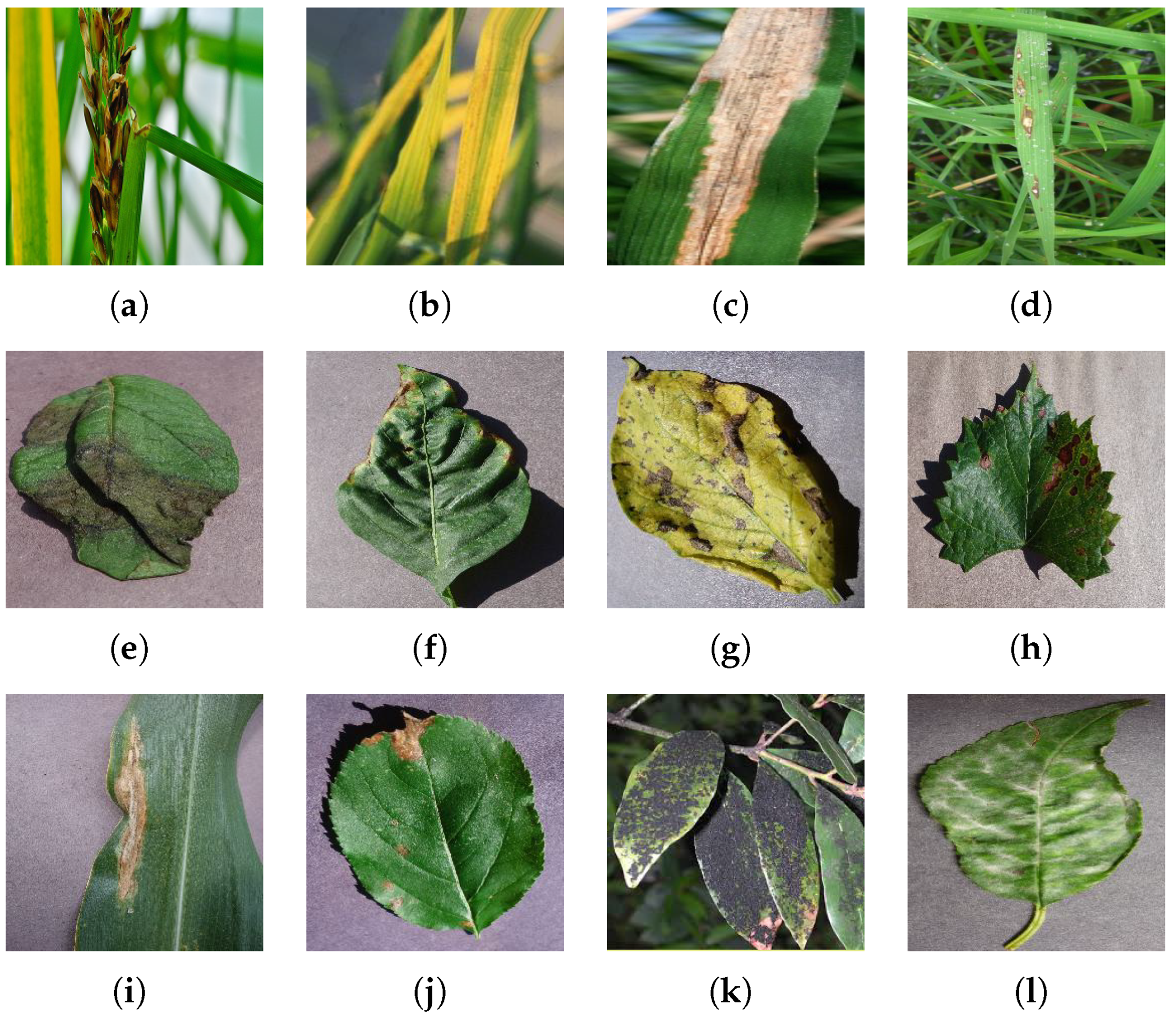
Symmetry 13 00511 g001
Figure 2. Samples of plant leaf disease images under numerous health conditions in various backgrounds and having different symptoms: (a) Rice Sheath-rot, (b) Rice Tungro, (c) Rice Bacterial leaf-blight, (d) Rice Blast, (e) Potato Late-blight, (f) Pepper Bacterial-spot, (g) Potato Early-blight Pepper Bacterial-spot, (h) Grape Black-measles, (i) Corn Northern Leaf-blight, (j) Apple Black-rot, (k) Mango Sooty-mold, and (l) Cherry Powdery-mildew.
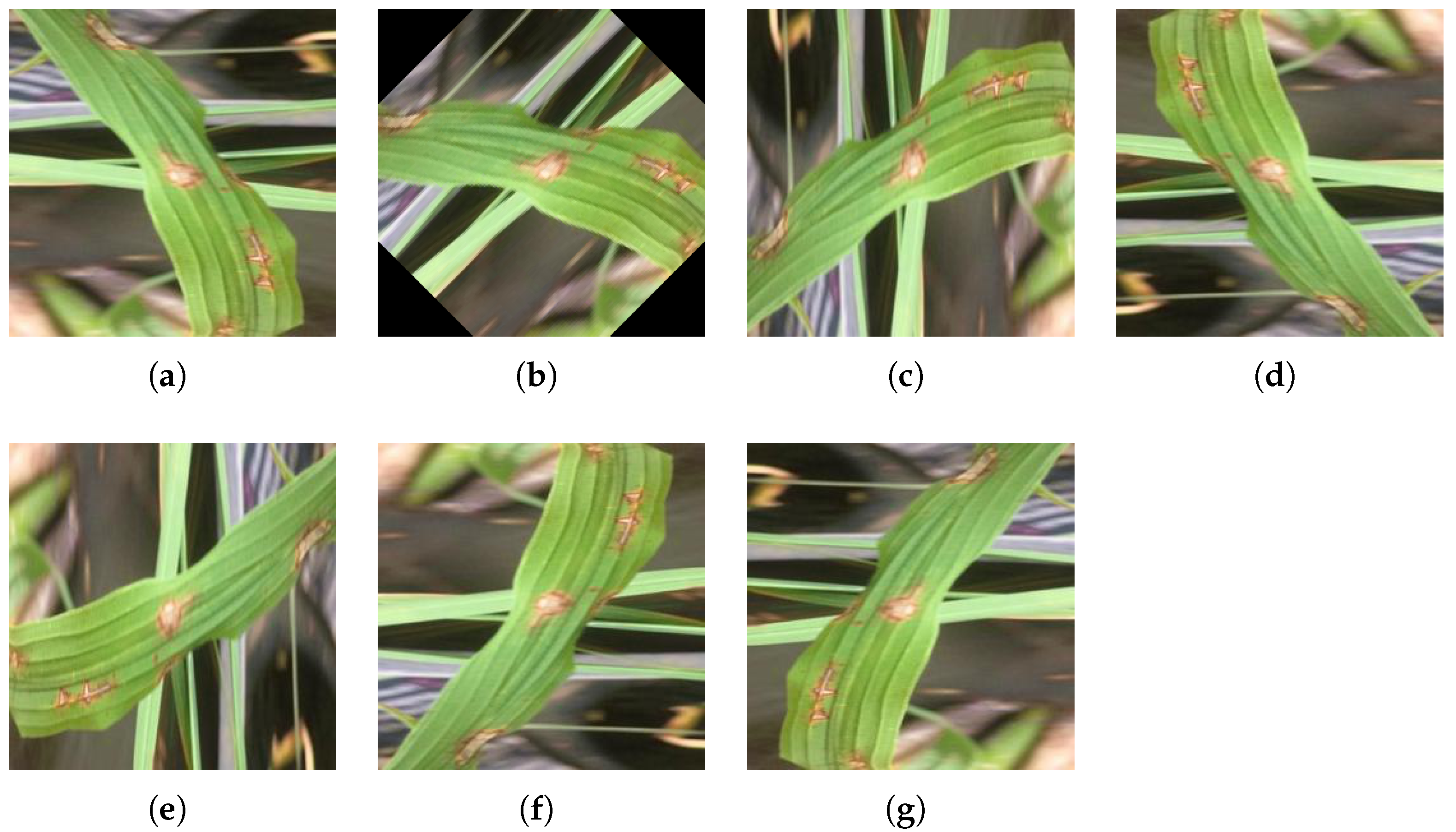
Symmetry 13 00511 g002
Figure 3. Directional Disturbance: (a) Original Rice Blast image. (b) Rotated by 45°. (c) Rotated by 90°. (d) Rotated by 180°. (e) Rotated by 270°. (f) Horizontal mirror symmetry. (g) Vertical mirror symmetry.
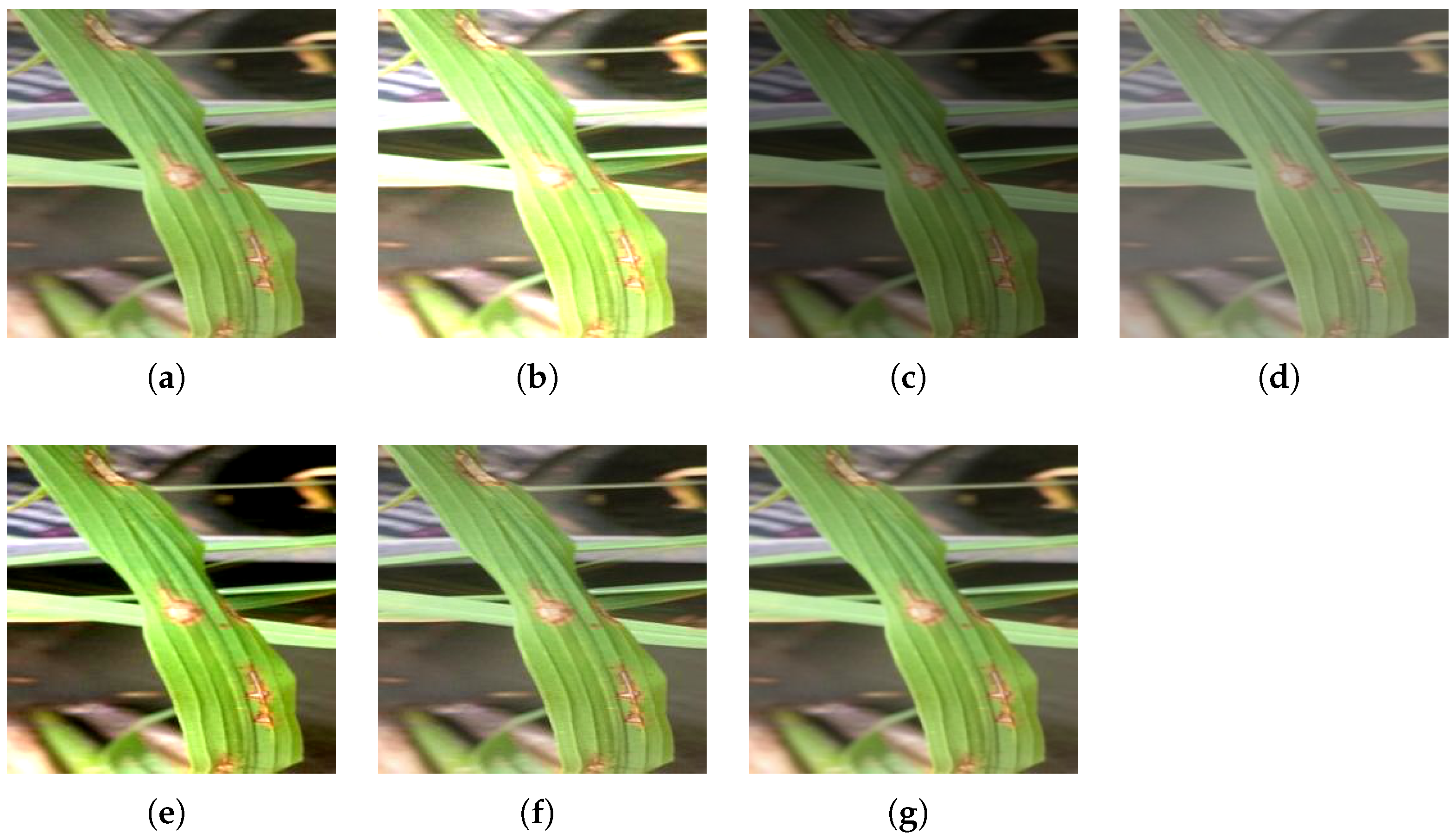
Symmetry 13 00511 g003
Figure 4. Illumination Disturbance: (a) Original Rice Blast image. (b) Brightened image. (c) Darkened image. (d) Less contrast image. (e) More contrast image. (f) Sharpened image. (g) Blur image.
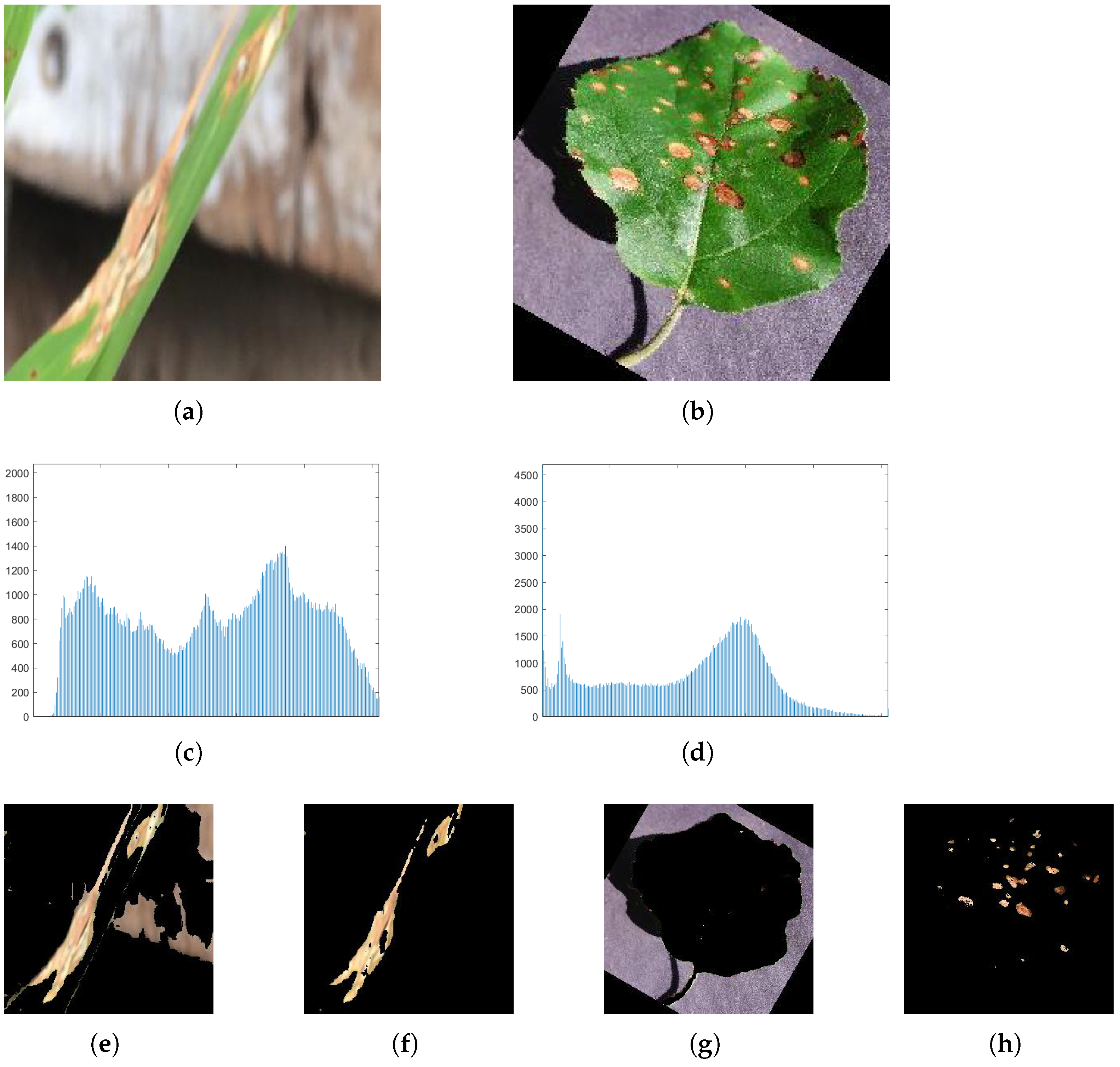
Symmetry 13 00511 g004
Figure 5. Effect of image enhancement on recognizing PLD: (a) rice blast disease image, and (b) apple black rot disease image. (c,d) are histogram of (a,b), respectively; (e,g) are the color segmentation results of (a,b), respectively, in traditional K-means clustering having extra noise without image enhancement, and (f,h) are the segmentation results of (a,b), respectively, in our modified color segmentation algorithm with image enhancement.
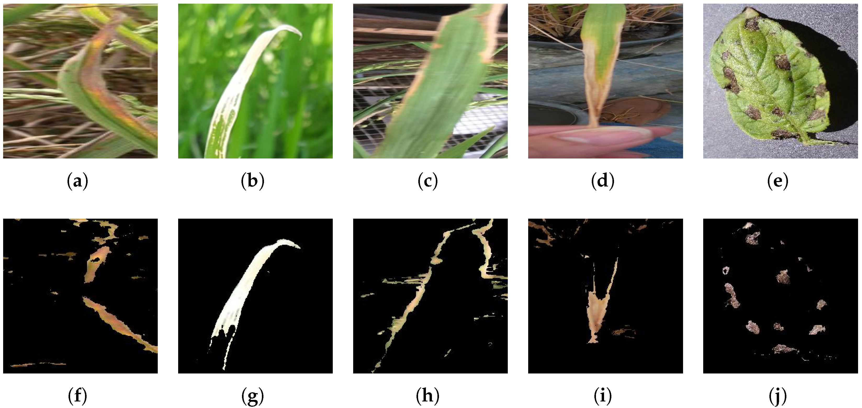
Symmetry 13 00511 g005
Figure 6. The effect of our modified segmentation technique under different critical environments: (ae) are the RGB PLD samples. (fj) are segmented regions of interest (ROIs) of (ae) after implementing adaptive centroid-based segmentation.
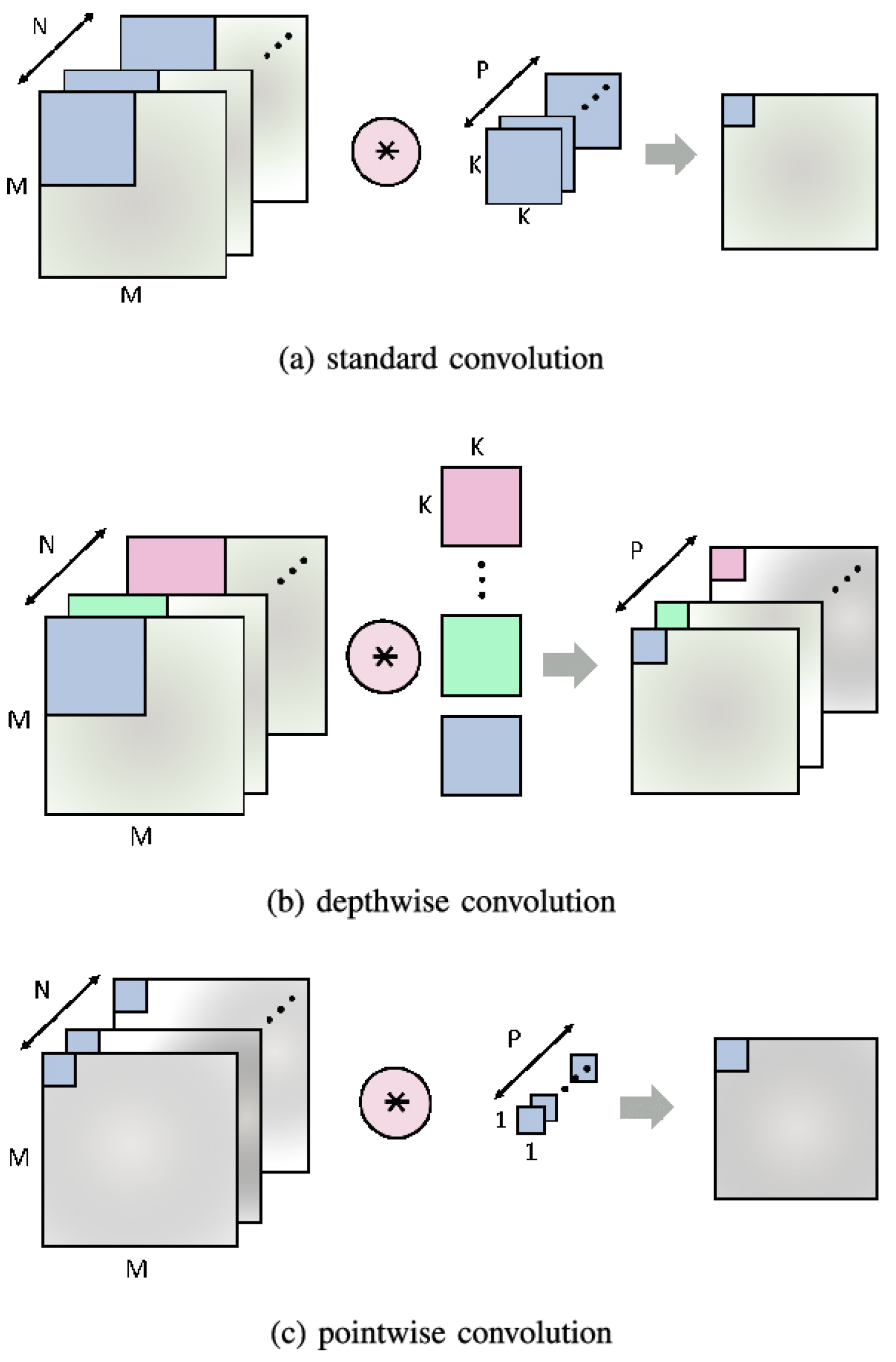
Symmetry 13 00511 g006
Figure 7. Comparison among various convolutions.
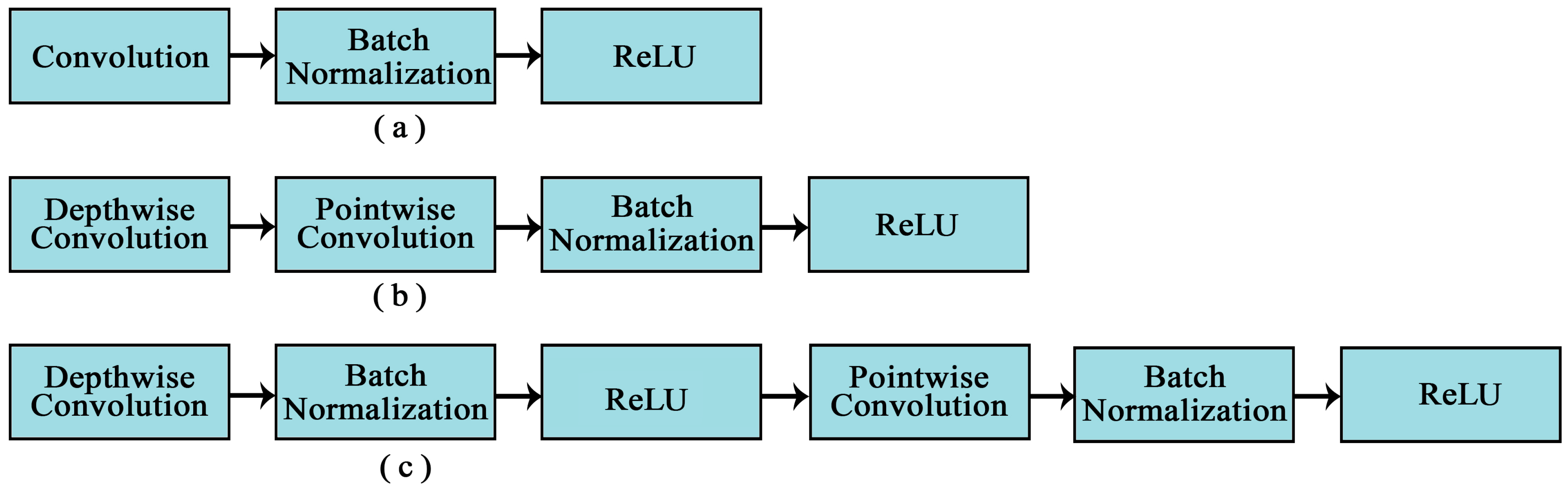
Symmetry 13 00511 g007
Figure 8. Primary modules for PLD recognition. (a) traditional convolutional layer, (b) quantization friendly depth-wise separable convolution, and (c) depth-wise separable convolution proposed in MobileNet.
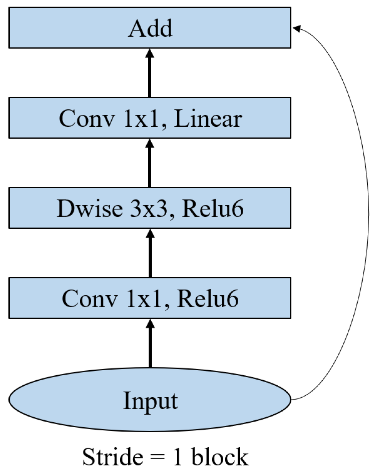
Symmetry 13 00511 g008
Figure 9. Primary module of MobileNetV2 for PLD recognition.
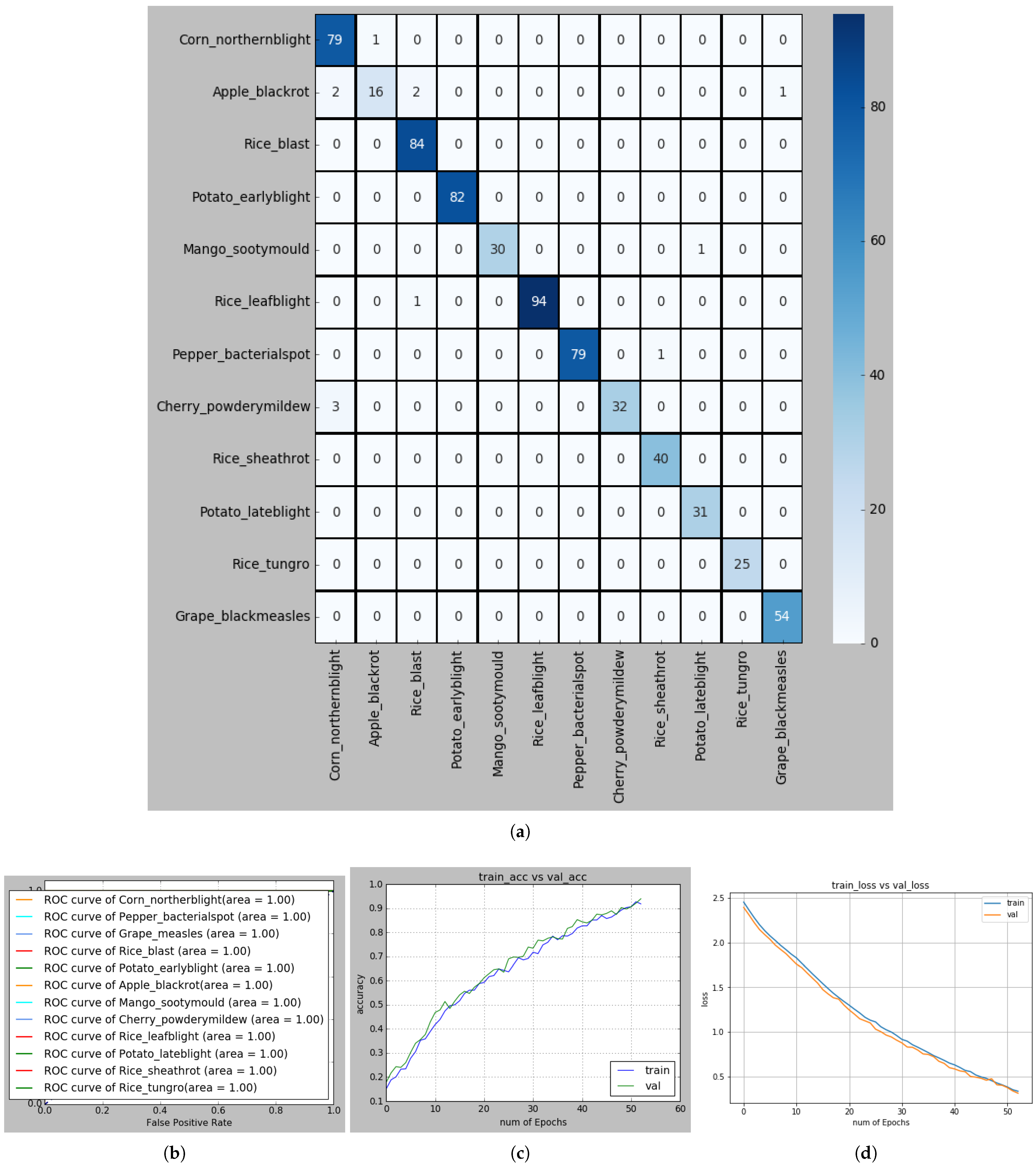
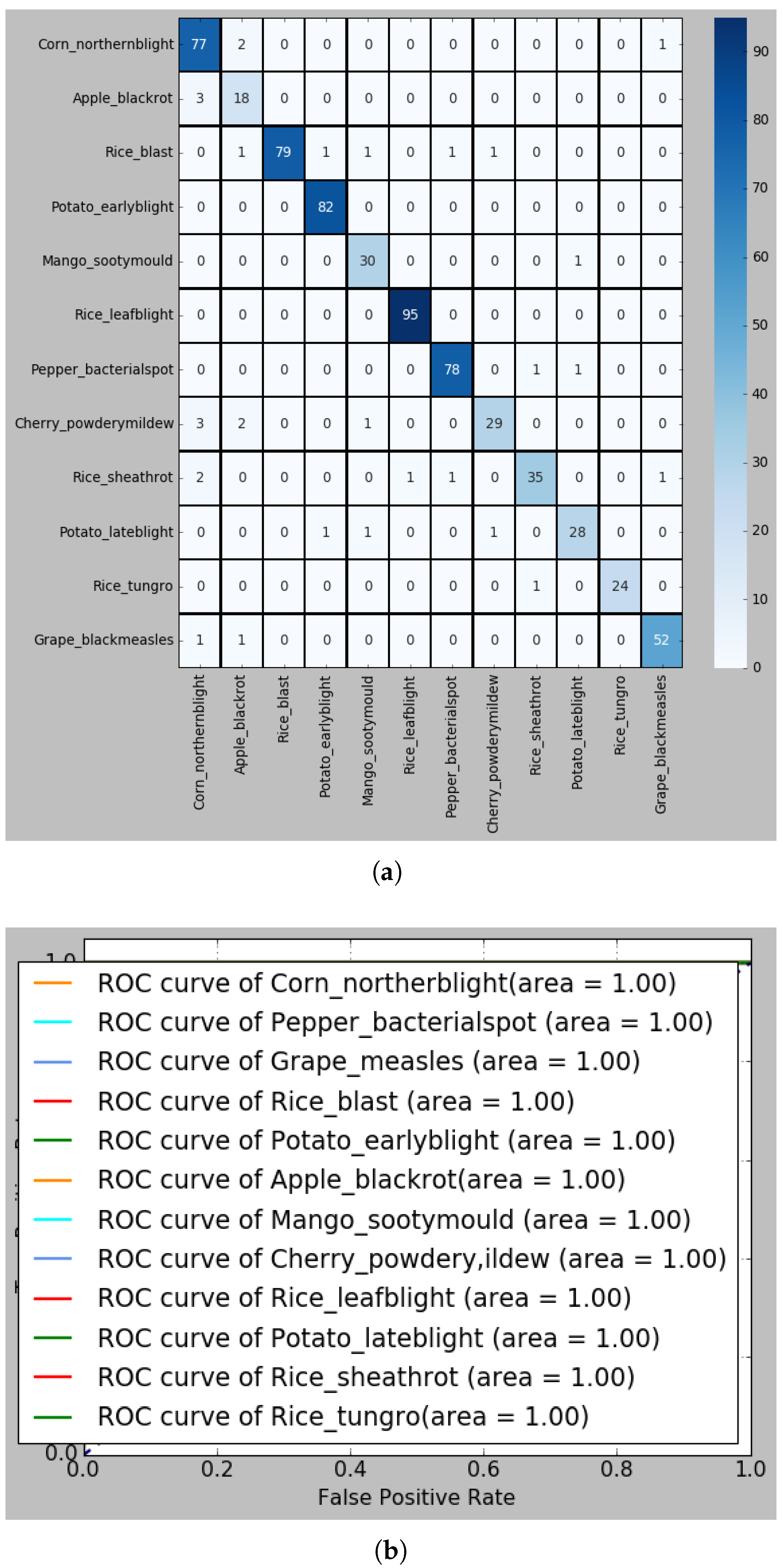
Symmetry 13 00511 g009
Figure 10. (a) Confusion matrix for recognizing PLDs; (b) ROC curve of each PLD; (c) Accuracy curve, and (d) Loss curve in S-modified MobileNet-based recognition framework.
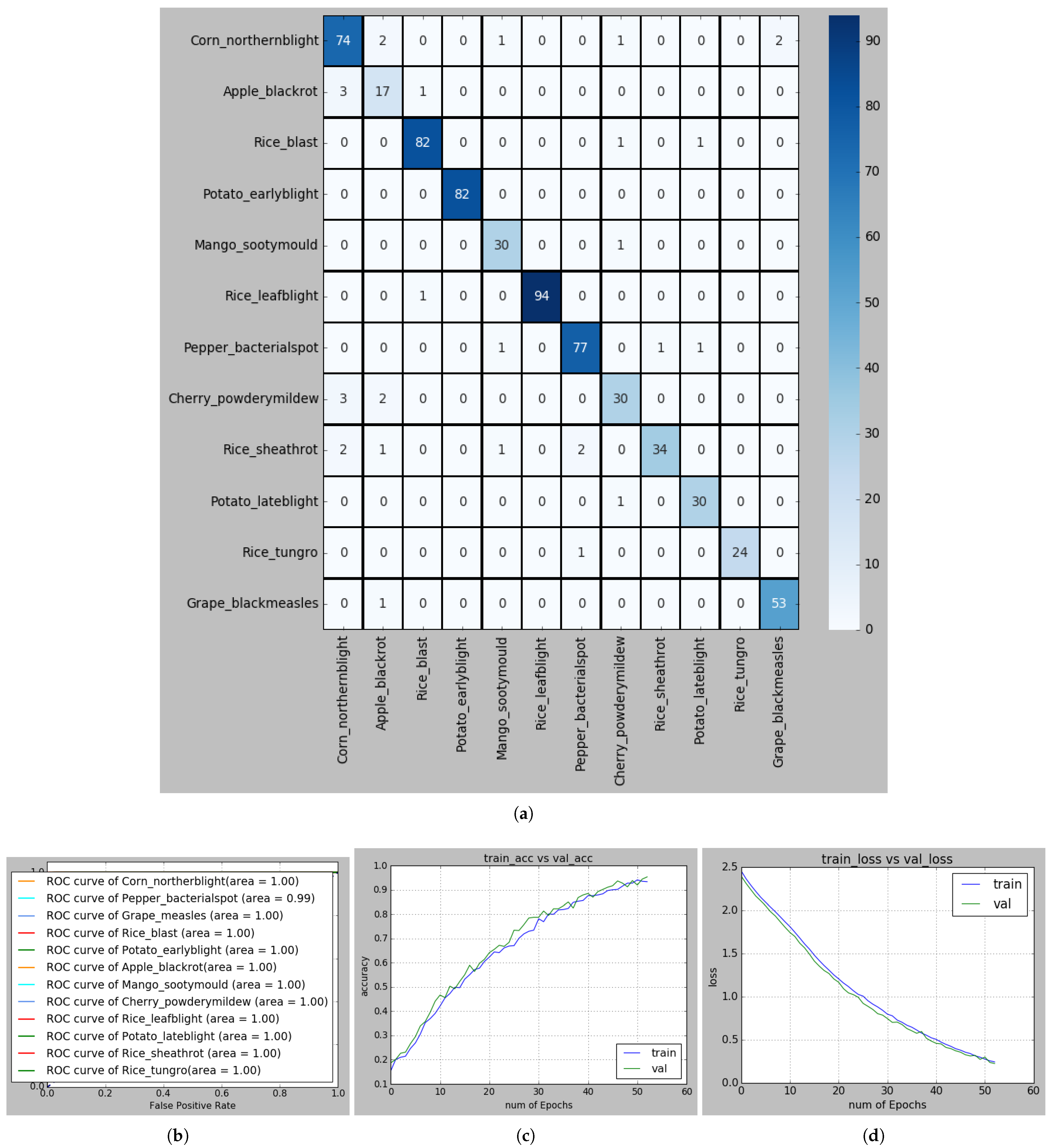
Symmetry 13 00511 g010
Figure 11. (a) Confusion matrix for recognizing PLDs; (b) ROC curve of each PLD; (c) Accuracy curve, and (d) Loss curve in S-reduced MobileNet-based recognition framework.
Symmetry 13 00511 g011
Figure 12. (a) Confusion matrix for recognizing PLDs; (b) ROC curve of each PLD; (c) Accuracy curve, and (d) Loss curve in S-extended MobileNet-based recognition framework.
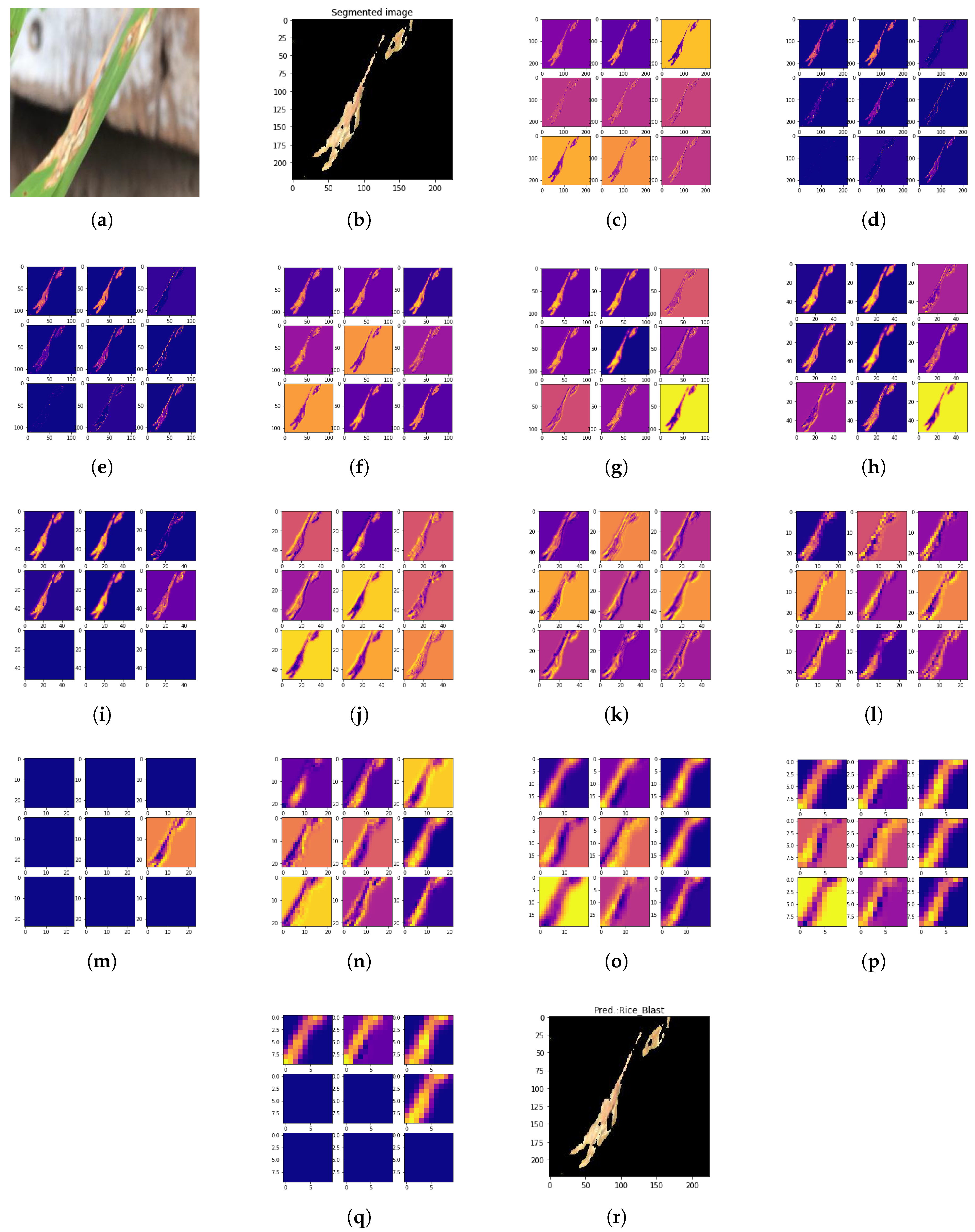
Symmetry 13 00511 g012
Figure 13. Processing steps of depth-wise separable convolutional PLD (DSCPLD) recognition framework using S-modified MobileNet: (a) Original Rice Blast image. (b) Segmented image after applying adaptive centroid-based segmentation (ACS). (c) Activations on the first CONV layer. (d) Activations on the first ReLU layer. (e) Activations on the first Max-pooling layer. (f) Activations on the first separable CONV layer. (g) Activations on the second separable CONV layer. (h) Activations on the second Max-pooling layer. (i) Activations on the second ReLU layer. (j) Activations on the third separable CONV layer. (k) Activations on the fourth separable CONV layer. (l) Activations on the third Max-pooling layer. (m) Activations on the third ReLU layer. (n) Activations on the fifth separable CONV layer. (o) Activations on the sixth separable CONV layer. (p) Activations on the fourth Max-pooling layer. (q) Activations on the fourth ReLU layer. and (r) Predicted result.
Symmetry 13 00511 g013
Figure 14. (a) Confusion matrix for recognizing PLDs and (b) ROC curve of each PLD in F-modified MobileNet-based recognition framework.
Symmetry 13 00511 g014
Table 1. Summary of some benchmark plant leaf disease (PLD) recognition frameworks.
ReferencesData Collected fromClasses/SpeciesNumber of ImagesData AugmentationCNN ArchitectureAccuracy
[6]PlantVillage58/2554,309YesVGG99.53%
[7]PlantVillage38/1454,306YesGoogleNet99.35%
[8]Collected15/64483YesModified CaffeNet96.30%
[10]PlantVillage38/1454,305YesDenseNet12199.75%
[11]Collected2/15808YesCustom95.83%
[13]PlantVillage3/13700YesModified LeNet92.88%
[14]Collected9/11426YesTwo stage CNN93.3%
[18]Collected4/11053YesModified AlexNet97.62%
[19]PlantVillage, Collected42/1279,265YesResNet15290.88%
[20]PlantVillage, Collected10/117929N/AF-CNN, S-CNN98.6%
[21]Collected7/17905YesCustom90.16%
[26]PlantVillage38/1454,323YesInceptionV399.76%
[28]Collected9/15000YesR-FCNN, ResNet5085.98%
[29]Collected56/141567YesGoogleNet94%
[30]Collected10/1500NoCustom95.48%
[31]Collected6/16029YesDenseNet+RF97.59%
Table 2. Limitations of some benchmark PLD recognition frameworks.
ReferencesFall in AccuracyComplex BackgroundMultiple Diseases in a SampleTrain and Test Data from Same DatasetComputational ComplexityMemory Restrictions
[6]NRNRPRNRNRNR
[7]NRNRNRNRNRNR
[8]NRRRNRNRNR
[10]NRNRNRNRNRNR
[11]NRNRNRNRNRNR
[13]NRNRNRNRNRNR
[14]NRPRNRNRNRR
[18]RNRNRNRNRNR
[19]RRRRRNR
[20]RRRRNRNR
[21]NRNRNRNRNRNR
[26]NRPRNRNRNRNR
[28]PRRRNRNRNR
[29]RPRNRNRNRNR
[30]NRPRNRNRNRNR
[31]NRRPRNRNRNR
NR = not resolved, R = resolved, PR = partially resolved.
Table 3. Dataset descriptions of plant leaf disease recognition.
Disease Class#Org. ImagesDistribution Techniques
TrainValidationTest
Corn_northern_blight80056016080
Pepper_bacterial_spot80056016080
Grape_black_measles54037810854
Rice_blast84058816884
Rice_bacterial_leaf_blight95066519095
Rice_sheath_rot4002808040
Rice_Tugro2501755025
Potato_early_blight82057416482
Potato_late_blight3102176231
Apple_black_rot2101474221
Mango_sooty_mold3102176231
Cherry_powdery_mildew3502457035
Total658046061316658
Table 4. S-modified MobileNet architecture for PLD recognition.
FunctionFilter/Pool#FiltersOutput#Parameters
Input-- 224 × 224 0
Convolution 3 × 3 32 32 × 222 × 222 896
Max pooling 2 × 2 - 32 × 111 × 111 0
Separable Convolution 3 × 3 64 64 × 109 × 109 2400
Separable Convolution 3 × 3 64 64 × 107 × 107 4736
Max pooling 2 × 2 - 64 × 53 × 53 0
Separable Convolution 3 × 3 128 128 × 51 × 51 8896
Separable Convolution 3 × 3 128 128 × 49 × 49 17,664
Max pooling 2 × 2 - 128 × 24 × 24 0
Separable Convolution 3 × 3 256 256 × 22 × 22 34,176
Separable Convolution 3 × 3 256 256 × 20 × 20 68,096
Max pooling 2 × 2 - 256 × 10 × 10 0
Global Average Pooling-- 1 × 1 × 256 0
Dense-- 1 × 1 × 1024 263,168
Dense-- 1 × 1 × 12 12,300
Softmax-- 1 × 1 × 12 0
Table 5. S-reduced MobileNet architecture for PLD recognition.
FunctionFilter/Pool#FiltersOutput#Parameters
Input-- 224 × 224 0
Convolution 3 × 3 32 32 × 222 × 222 896
Depth-wise Convolution 3 × 3 32 32 × 64 × 64 32,800
Point-wise Convolution 1 × 1 64 64 × 64 × 64 2112
Depth-wise Convolution 3 × 3 64 64 × 1 × 1 262,208
Point-wise Convolution 1 × 1 128 128 × 1 × 1 8320
Global Average Pooling-- 1 × 1 × 128 0
Dense-- 1 × 1 × 12 1548
Softmax-- 1 × 1 × 12 0
Table 6. S-extended MobileNet architecture for PLD recognition.
FunctionFilter/Pool#FiltersOutput#Parameters
Input-- 256 × 256 0
Convolution 3 × 3 32 32 × 254 × 254 896
Depth-wise Convolution 3 × 3 32 32 × 75 × 75 32,800
Point-wise Convolution 1 × 1 64 64 × 75 × 75 2112
Depth-wise Convolution 3 × 3 64 64 × 4 × 4 262,208
Point-wise Convolution 1 × 1 128 128 × 4 × 4 8320
Max pooling 2 × 2 - 128 × 2 × 2 0
Dense-- 1 × 1 × 1024 5,25,312
Dense-- 1 × 1 × 12 12,300
Softmax-- 1 × 1 × 12 0
Table 7. Hyper-parameters used in various models for PLD recognition.
Hyper-ParametersSGDAdamRMSprop
Epochs50–15050–15050–150
Batch size32, 6432, 6432, 64
Learning rate0.0010.001, 0.00010.0001
β 1 -0.9-
β 2 -0.999-
Momentum0.8, 0.9--
Table 8. Source-wise dataset distribution summary.
SourcesSpeciesDiseasesNo. of Training ImagesNo. of Validation ImagesNo. of Test ImagesNo. of Training Images (Source-Wise)No. of Validation Images (Source-Wise)No. of Test Images (Source-Wise)
PlantVillagepepperBacterial-spot5601608028981459414
PotatoEarly-blight57416482
Late-blight2176231
CornNorthern-blight56016080
MangoSooty-mold2176231
AppleBlack-rot1474221
CherryPowdery-mildew2457035
GrapeBlack-measles37810854
KaggleRiceBlast588168841253358179
Bacterial leaf-blight66519095
IRRI/BRRI/
other sources
RiceSheath-rot280804045513065
Tungro1755025
Total images 46061316658
Table 9. A concrete representation of accuracies and mean F1-score of various PLD recognition models using segmented images.
ModelsTraining AccuracyValidation AccuracyMean Test AccuracyMean F1-Score
VGG1699.91%99.53%99.21%96.74%
VGG1999.93%99.53%99.39%96.91%
AlexNet99.07%98.82%98.78%96.31%
MobileNetV199.93%99.41%99.24%95.67%
MobileNetV299.96%99.82%99.41%96.07%
MobileNetV3100%99.89%99.55%96.97%
S-extended MobileNet99.78%99.31%98.37%95.92%
S-reduced MobileNet99.93%99.70%99.41%96.93%
S-modified MobileNet100%99.70%99.55%97.07%
Table 10. A concrete representation of computational latency and model size of various PLD recognition models using segmented images.
ModelsImage SizeFLOPsMACC# Parameters
VGG16 180 × 180 213.5 M106.75 M15.2 M
VGG19 180 × 180 287.84 M143.92 M20.6 M
AlexNet 224 × 224 127.68 M63.84 M6.4 M
MobileNetV1 224 × 224 83.87 M41.93 M3.2 M
MobileNetV2 224 × 224 81.91 M40.96 M1.61 M
MobileNetV3 224 × 224 59.8 M29.90 M3.2 M
S-extended MobileNet 256 × 256 16.86 M8.43 M0.84 M
S-reduced MobileNet 224 × 224 3.70 M2.15 M0.31 M
S-modified MobileNet 224 × 224 5.78 M2.89 M0.41 M
Table 11. Various accuracies and mean F1-score of PLD models using full leaf images.
ModelsTraining AccuracyValidation AccuracyMean Test AccuracyMean F1-Score
VGG1699.78%99.39%98.78%96.32%
VGG1999.78%99.41%99.01%96.54%
AlexNet98.71%98.64%98.34%95.89%
MobileNetV199.81%99.43%98.79%96.54%
MobileNetV299.89%99.53%98.99%96.56%
MobileNetV399.91%99.53%99.05%96.58%
F-extended MobileNet99.58%99.21%98.14%95.22%
F-reduced MobileNet99.91%99.58%99.07%96.60%
F-modified MobileNet99.91%99.63%99.10%96.63%
Table 12. Performance comparison of each disease using S-modified MobileNet and F-modified MobileNet.
ClassS-modified MobileNetF-modified MobileNet
Accuracy (%)F1-Score (%)Accuracy (%)F1-Score (%)
Corn_northern_blight99.0896.3498.1892.77
Pepper_bacterial_spot99.8599.3799.3997.50
Grape_black_measles99.8599.0899.3996.30
Rice_blast99.5498.2499.2496.93
Potato_early_blight10010099.7098.87
Apple_black_rot99.0884.2498.6380
Mango_sooty_mold99.8598.3699.3993.75
Cherry_powdery_mildew99.5495.5298.7887.88
Rice_bacterial_leaf_blight99.8599.4599.8599.45
Potato_late_blight99.8598.4199.2491.80
Rice_sheath_rot99.8598.7698.9491.02
Rice_Tugro10010099.8597.96
Total99.5597.0799.1096.63
Table 13. Performance comparison of each disease using S-reduced MobileNet and F-reduced MobileNet.
ClassS-reduced MobileNetF-reduced MobileNet
Accuracy (%)F1-Score (%)Accuracy (%)F1-Score (%)
Corn_northern_blight98.6394.5498.1892.77
Pepper_bacterial_spot99.0899.3899.3997.50
Grape_black_measles99.5498.1599.3996.30
Rice_blast99.5498.1899.2496.93
Potato_early_blight99.8599.4099.7098.87
Apple_black_rot98.9483.7298.6380
Mango_sooty_mold99.8598.3699.3993.75
Cherry_powdery_mildew98.6397.0798.7897.88
Rice_bacterial_leaf_blight99.8599.4899.8599.45
Potato_late_blight99.5496.8899.2491.80
Rice_sheath_rot98.9393.3397.8598.05
Rice_Tugro10010099.8597.96
Total99.4196.9399.0796.60
Table 14. Performance comparison of each disease using S-extended MobileNet and F-extended MobileNet.
ClassS-extended MobileNetF-extended MobileNet
Accuracy (%)F1-Score (%)Accuracy (%)F1-Score (%)
Corn_northern_blight97.8791.3697.1890.67
Pepper_bacterial_spot99.0896.2598.7997.50
Grape_black_measles99.5497.2599.3996.30
Rice_blast99.3997.6299.2496.93
Potato_early_blight10010099.7098.87
Apple_black_rot98.4873.0697.0370.03
Mango_sooty_mold99.3995.2499.3993.75
Cherry_powdery_mildew98.6386.9697.7887.88
Rice_bacterial_leaf_blight99.8599.4799.8599.45
Potato_late_blight99.5495.2499.2490.67
Rice_sheath_rot98.9390.6797.8588.05
Rice_Tugro99.8497.9699.8597.96
Total98.3795.9298.1495.22
Table 15. A concrete representation of experiments on MobileNetV3 with width multipliers.
ModelsMean Test AccuracyMean F1-ScoreFLOPsMACC# Parameters
0.25 MobileNetV3-22495.48%93.39%4.30 M2.15 M0.38 M
0.5 MobileNetV3-22497.78%95.01%15.66 M7.83 M0.99 M
0.75 MobileNetV3-22498.81%95.64%34.16 M17.08 M1.98 M
1.0 MobileNetV3-22499.55%96.97%59.8 M29.90 M3.2 M
Table 16. A concrete representation of experiments on MobileNetV3 with resolutions.
ModelsMean Test AccuracyMean F1-ScoreFLOPsMACC# Parameters
1.0 MobileNetV3-12896.88%95.39%19.55 M9.77 M3.2 M
1.0 MobileNetV3-16099.08%95.78%30.48 M15.24 M3.2 M
1.0 MobileNetV3-19299.31%96.64%43.93 M21.97 M3.2 M
1.0 MobileNetV3-22499.55%96.97%59.8 M29.90 M3.2 M
Table 17. Performance evaluation trained on our dataset using S-modified MobileNet and test on different datasets using various optimizers.
DatasetSGDAdamRMSprop
Rice dataset98.25%97.05%98.53%
Our PLD dataset99.31%99.39%99.55%
Table 18. Performance evaluation trained on our dataset using F-modified MobileNet and test on different datasets using various optimizers.
DatasetSGDAdamRMSprop
Rice dataset90.65%92.25%95.53%
Our PLD dataset98.39%98.53%99.10%
Table 19. Comparison among some benchmark PLD recognition frameworks.
ReferencesClasses/SpeciesCNN ArchitectureFall in AccuracyComputational ComplexityMemory RestrictionAccuracy
[6]58/25VGGNRNRNR99.53%
[7]38/14GoogleNetNRNRNR99.35%
[8]15/6Modified CaffeNetNRNRNR96.30%
[11]2/1CustomNRNRNR95.83%
[13]3/1Modified LeNetNRNRNR92.88%
[14]9/1Two stage CNNNRNRR93.3%
[18]4/1Modified AlexNetRNRNR97.62%
[19]42/12ResNet152RRNR90.88%
[20]10/1F-CNN, S-CNNRNRNR98.6%
[21]7/1CustomNRNRNR90.16%
[28]9/1R-FCNN, ResNet50PRNRNR85.98%
[29]56/14GoogleNetRNRNR94%
[30]10/1CustomNRNRNR95.48%
[31]6/1DenseNet+RFNRNRNR97.59%
Our work12/8S-modified MobileNetRRR99.55%
NR = not resolved, R = resolved, PR = partially resolved.
Publisher’s Note: MDPI stays neutral with regard to jurisdictional claims in published maps and institutional affiliations.

