Abstract
In this paper, we present a new Fuzzy Implication Generator via Fuzzy Negations which was generated via conical sections, in combination with the well-known Fuzzy Conjunction. The new Fuzzy Implication Generator takes its final forms after being configured by the fuzzy strong negations and combined with the most well-known fuzzy conjunctions , , , , and . The final implications that emerge, given that they are configured with the appropriate code, select the best value of the parameter and the best combination of the fuzzy conjunctions. This choice is made after comparing them with the Empiristic implication, which was created with the help of real temperature and humidity data from the Hellenic Meteorological Service. The use of the Empiristic implication is based on real data, and it also reduces the volume of the data without canceling them. Finally, the MATLAB code, which was used in the programming part of the paper, uses the new Fuzzy Implication Generator and approaches the Empiristic implication satisfactorily which is our final goal.
1. Motivation
The motivation for writing this paper was the construction of flexible fuzzy implications via strong negations and their application to real data collected from the thirteen regions of Greece in the last five years 2015–2019 by the Hellenic Meteorological Service (see Reference [1]). Most publications or literature dealing with evolving systems (see Reference [2,3,4]) use mostly fuzzy systems or Generalized Fuzzy Rules without the use of fuzzy negations (for Fuzzy Negations, see Reference [5,6,7]). It was, therefore, a research challenge to study whether negations and especially fuzzy negations with a parameter, such as Sugeno class, and Yager class (see Example 2 and Reference [8]) can be used in fuzzy implications by lending their parameter to fuzzy rules (if… then…). The configuration of fuzzy rules creates flexible fuzzy implications since, by changing the parameter, the implication changes, as well. As a result, an algorithm for finding the best implication emerges by changing the parameter. The best implication is found through the square error of the empiristic implication (see Section 4.1).
2. Introduction
The Theory of Fuzzy Implications and Fuzzy Negations plays an important role in many applications of fuzzy logic, such as approximate reasoning, formal methods of proof, inference systems, and decision support systems (see References [9,10]). Recognizing the above important role of Fuzzy Implications and Fuzzy Negations, we tried to construct Fuzzy implications from Fuzzy negations, so that we could change the implication with one parameter, thus giving an algorithmic procedure of the “if……then……” rule. The tools for this construction, namely a fuzzy implication generator, were mainly the conclusions of Souliotis G.’s and Papadopoulos B.’s paper [8] (p. 5) and, in particular, the following Equation (1):
producing fuzzy negations via conical sections and Corollary 2.5.31 (see Reference [11]).The combination of these two, through the fuzzy conjunction basic t-norm (see Table 1), gave us an algorithmic procedure for the evaluation of the best implication with respect to the problem data. For the evaluation of the best implication, the Empiristic implication was used (see Reference [12]) as a comparison measurement. The Empiristic implication does not satisfy any of the properties of the fuzzy implications and has no specific formula, meaning it is not a function. However, the choice of this particular implication was not random as it was based on its ability to be directly calculated by the empirical data without being affected by the amount of the data.

Table 1.
Basic t-norms.
The paper follows the following structure:
The section “Preliminaries” presents the theoretical background of the paper, such as the definitions of the Fuzzy Implications, Fuzzy Negations, and Triangular norms.
The section “Main Results” shows the table of the Empiristic implication and the algorithm for its calculation. The data used, such as the average monthly temperature and the average monthly relative humidity, two of the most important environmental variables in meteorology (see Reference [1]), are real. Next, the parametric implications which are constructed by a strong fuzzy negation, the basic t-norm (see Table 1), the table of the parametric implications and the algorithms for its calculations are presented. Furthermore, the algorithmic process for finding the best fuzzy implication among the Empiristic implication, the three known implications from the literature (Kleen-Dienes, Lukasiewicz, Reichenbach) (see Reference [11]) and the constructed parametric implications are analysed. The calculation of the implications with the use of data was done in the MATLAB programming environment. Finally, the code and the documentation of the MATLAB, which was used to calculate the implications, are presented.
3. Preliminaries
A prerequisite for the understanding of the paper by its reader is the preliminary data that we must cite about the fuzzy negations, the fuzzy conjunctions and the fuzzy implications. A fuzzy implication is a generalization of the classical one to fuzzy logic, much in the same way as a t-norm and a t-conorm are generalizations of the classical conjunction and disjunction, respectively. In this section, we give the basic definitions and examples of fuzzy implications. Next, we introduce some main properties of fuzzy implications and their inter-dependencies with fuzzy negations.
3.1. Fuzzy Implication
In the literature, we can find several different definitions of fuzzy implications. In this paper, we will use the following one, which is equivalent to the definition proposed by Kitainik [13] (also see Reference [10,11]).
Definition 1.
A function is called a fuzzy implication if, for all , the following conditions are satisfied:
Example 1.
In Baczyński’s book, p. 4, Table 1.3 (see Reference [11]), can be found some examples of Fuzzy Implications:
Kleene-Dienes:
Lukasiewicz:
Reichenbach:
3.2. Fuzzy Negations
The following definitions and examples can be found [11,14,15,16].
Definition 2.
A function is called a Fuzzy negation if
Definition 3.
A fuzzy negation N is called strict if, in addition,
(N3) N is strictly decreasing,
(N4) N is continuous,
A fuzzy negation N is called strong if the following property is met,
Example 2.
In Baczyński’s book, p. 15, Table 1.6 (see Reference [11]), can be found some examples of Fuzzy Negations:
Remark 1.
In Souliotis G.’s and Papadopoulos B.’s paper [8], p. 5 proves a new family of strong fuzzy negations, which is produced by conical sections and is given from Equation (1), which will play a key role in building the algorithmic procedure we propose in the section “Main Results”.
3.3. Triangular Norms (Conjunctions)
The Triangular norms were introduced by Menger [16] and were later reconstructed by Schweizer and Sklar [17] in the form they have today. In essence, they are a generalization of the classical binary conjunction into a fuzzy intersection. The following definition can be found in the monograph by Klement et al. [18] (also see Reference [11]).
Definition 4.
(see Reference [16]). A function is called triangular norms shortly t- norm, if it satisfies, for all , the following conditions:
Table 1 lists a few of the common t-norms.
4. Main Results
The main part of the paper consists of three parts. The creation of the empiristic implication that is presented with the construction of a table after first dividing the data into classes. Furthermore, the theoretical part includes the mathematical process by which the parametric implications were created via strong fuzzy negations. Then the practical part of the work that includes the programming part (see MATLAB code [19,20]) with which the empiristic is compared with the parametric implication using real environmental data of temperature and relative humidity.
4.1. Construction of the Table of the Empiristic Implication
The steps for constructing the Empiristic implication table are:
Step 1
The data of the temperature and the humidity of the last five years 2015–2019 (see Reference [1]) were classified in ascending order (Figure 1).
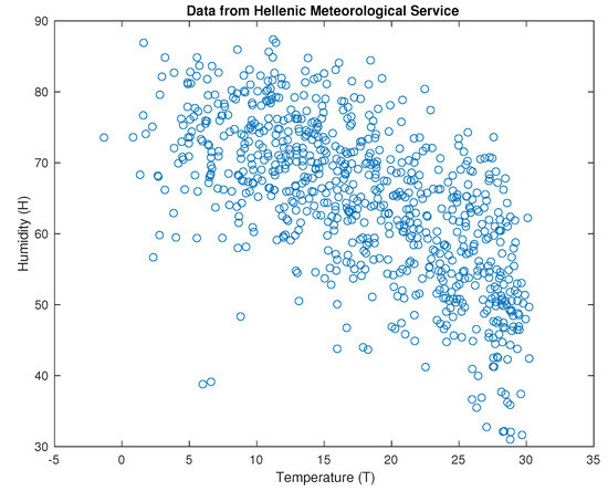
Figure 1.
Data from the Hellenic Meteorological Service (see Reference [1]).
Step 2
Fuzzy sets with Gaussian membership functions were used in order to be normalized between the values [0, 1]. The language variables used were low, medium and high for the temperature and the humidity, respectively.
The language rules used were the following:
- Low temperature means High humidity.
- Medium temperature means Medium humidity.
- High temperature means Low humidity.
Remark 2.
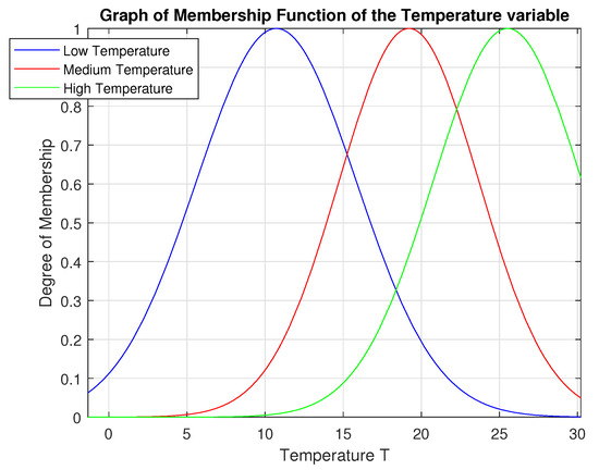
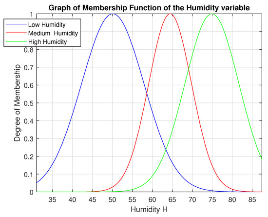
Gauss membership functions that were used to normalize the data were not chosen randomly. They resulted from the classification of the data, as well as the appropriate application of the MATLAB code (see Figure 2 and Figure 3).
Figure 2.
The Membership Function of the Temperature Variable is the Gaussian membership functions , from which the standard deviation, σ, and mean, c are gaussmf[5.122 10.72], gaussmf[4.481 19.21], gaussmf[4.768 25.52], respectively.
Figure 3.
Membership Function of the Humidity Variable is Gaussian membership functions , from which the standard deviation, σ, and mean, c are gaussmf[7.826 50.09], gaussmf[5.371 64.44], gaussmf[6.775 74.89], respectively.
Step 3
Then, the data were divided into 11 classes applying the Sturges formula: , where n is multitude of data [(13 regions).(12 months).(5 years) = 780].
c = 10.6 rounding c = 11 classes.
Step 4
Next, the medians of the above classes were calculated.
Step 5
This resulted in a 12 × 12 table which includes the medians of the humidity classes in the 1st row and the medians of the temperature classes in the 1st column (see Table 2).
Table 2.
Final Table.
Step 6
We assumed we wanted to fill in the cell (1,10) of the above table. The pairs of the data in which their temperatures belong to the 1st class and the humidities to the 10th class were checked.
Step 7
After this check 14 pairs were found to meet the above requirement, as shown in the table above (see Table 3).
Table 3.
Cell (1, 10).
Step 8
The table was completed with a similar procedure.
Step 9
The resulting number for each cell was divided by the sum of the corresponding column where it belongs.
Step 10
From the above procedure, a new table 11 × 11 derived, which is the table of the Empiristic implication (see Table 4).
Table 4.
Table of the Empiristic Implication.
4.2. Generated Parametric Fuzzy Implications
Theorem 1.
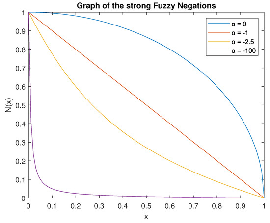
In Baczyński’s book (see Reference [11]), particularly p. 87, in Corollary (2.5.31), the implication
generated by a strong fuzzy negation . In Figure 4, which is visible below, is presented the graph of the equation N(x) for four random values of the parameter α and a t-norm (Minimum T norm):
It produces Equation (5).
Figure 4.
Graph of the strong Fuzzy Negations Ν(x) for four random values of the parameter .
Proof.
□
Theorem 2.
If, in Theorem 1, t-norm gets replaced by t-norm (Algebraic product T norm)
it produces Equation (7).
Proof.
□
Theorem 3.
If, in Theorem 1, t-norm gets replaced by t-norm (Lukasiewicz T norm):
it produces Equation (9).
Proof.
□
Theorem 4.
If, in Theorem 1, t-norm gets replaced by t-norm (Active product T norm)
it produces Equation (11).
Proof.
□
Theorem 5.
If, in Theorem 1, t-norm gets replaced by t-norm (Nilpotent minimum T norm)
it produces Equation (13).
Proof.
□
4.3. Construction of the Table of the Parametric Fuzzy Implication
The steps for constructing the parametric implication table are: The procedure that was followed for the construction of the table is the same which was used in the first five steps for the construction of the Empiristic implication table. More specifically:
Step 1
The data of the temperature and the humidity of the last five years 2015–2019 [1] were classified in ascending order (Figure 1).
Step 2
Fuzzy sets with Gaussian membership functions were used in order to be normalized between the values [0, 1]. The language variables used were low, medium, and high for the temperature and the humidity, respectively.
The language rules used were the following:
- Low temperature means High humidity.
- Medium temperature means Medium humidity.
- High temperature means Low humidity.
Step 3
Then, the data were divided into 11 classes applying the Sturges formula: .
Step 4
Next, the medians of the above classes were calculated.
Step 5
This resulted in a 12 × 12 table which includes the medians of the humidity classes in the 1st row and the medians of the temperature classes in the 1st column.
Step 6
The parametric implication of Equation(5), Equation (7), Equation (9), Equation (11), Equation (13) is applied and the minimum square error between the Empiristic implication table, and the parametric implication table emerges.
4.4. Find the Most Appropriate Parametric Fuzzy Implications
4.4.1. The Control of the Norm of the Empiristic and Three Well Known Implications (see Example 1).
- The squared error of the two implications (Empiristic and Kleen-Dienes) gives the result is 8.4922.
- The squared error of the two implications (Empiristic and Lukasiewicz) gives the result is 9.1654.
- The squared error of the two implications (Empiristic and Reichenbach) gives the result is 8.6690.
4.4.2. The Control of the Norm of the Empiristic and Parametric Implication
First of all the data have been classified in clusters by using the method Fuzzy c-means (FCM) [6]. Fuzzy c-means (FCM) is a data clustering technique where each data point belongs to a cluster to some degree that is specified by a membership grade (Figure 5) (see Reference [19,20], A.4).

Figure 5.
Data in Clusters.
To generate a Mamdani-type fuzzy inference system that models the behavior of input/output data, you can configure the genfis command to use FCM clustering. Using the Mamdani-type fuzzy inference system, the Gaussian membership functions for input and output of the data were found. The Gaussian membership functions were utilized to normalize the data of the tables of the parametric implications (see Reference [19,20], A.4, A.4.1, and A.5)
Description the MATLAB code for the Control between Empiristic and Parametric Implication
Step 1
The data are loaded after classification.
Step 2
A column which is the increment number, is added to this table in order not to miss the original pairs (xi, yi). The column added is the third one.
Step 3
Later, a different table for X, together with its increment number, and a different one for Y are created.
Step 4
Then, the initial position for each X and Y emerges, so we sort in ascending order according to the values. We notice that, in the first column, we have X and Y in ascending order and, in the second column, their positions.
Step 5
We normalize using Gaussian membership functions.
Step 6
The Sturges formula, , is applied in order to distinguish in classes the sorted data columns.
Step 7
Next, 11 classes are created for each sorted table.
Step 8
The classes are added to the third column in the sorted tables. The format of the sorted tables is: the first column has X in ascending order, the second column has the initial position, and the third column has the class.
Step 9
Then, the above two tables are sorted by increment number to get the data back to their original position, along with their classes.
Step 10
The above tables are placed in a table where the first column is X, the second is the class of X, the third is Y, and the fourth is the class of Y.
Step 11
A Zero Table is created. The table will be a column larger and a column smaller to place the medians.
Step 12
Finally, the table we want emerges without adding values to the first row and column.
Step 13
Medians are created for the classes of Y and are placed in the Final Table.
Step 14
The Final Table has the medians of the classes of Y as its first row and the medians of the classes of X as its first column. A new table with zeros is created.
Step 15
The table of the Empiristic implication is created.
Step 16
The Other Table is the table of the parametric implication.
Step 17
In the next step, the parametric implication is introduced. The parameter implication is defined as The value of the parameter a, for which we have the minimum norm, is found.
Remark 3.
The control of the norm of the Empiristic and Parametric implication.
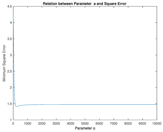
The squared error of the two implications (Empiristic and Parametric (5) gives the result is 1.4127 and parameter (see Reference [19,20], A.5, and Figure 6).
Figure 6.
Relation between Parametric (5) and Square Error.
The same steps were followed for the control of the Empiristic and the Parametric implications using our MATLAB codes (see Reference [19,20], A.5, A.6, A.7, A.8, and A.9), with the only difference being, the replacement of the appropriate equation that describes the parametric implication.
Particularly:
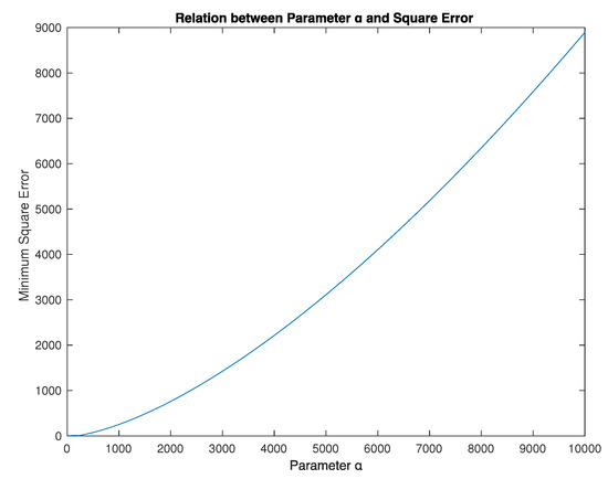
The squared error of the two implications (Empiristic and Parametric (7)) gives the result is 3.4870 and parameter (see Reference [19,20], A.6, and Figure 7).
Figure 7.
Relation between Parametric (7) and Square Error.
The squared error of the two implications (Empiristic and Parametric (9)) gives the result is 8.9889 and parameter (see Reference [19,20], A.7, and Figure 8).
Figure 8.
Relation between Parametric (9) and Square Error.
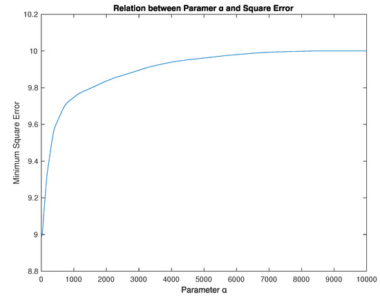
The squared error of the two implications (Empiristic and Parametric (11)) gives the result is 3.1892 and parameter (see Reference [19,20], A.8, and Figure 9).
Figure 9.
Relation between Parametric (11) and Square Error.
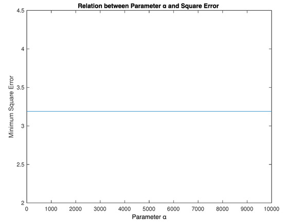
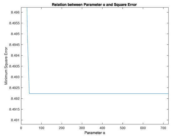
The squared error of the two implications (Empiristic and Parametric (13)) gives the result is 8.4922 and parameter (see Reference [19,20], A.9, and Figure 10).
Figure 10.
Relation between Parametric (13) and Square Error.
After the examination of the three well known implications (see Example 1) is completed and the examination of the five parametric, we proceed to find the best parameter that we have from the (5). We have the best approach for the value and with a very good approach the squared error of the two implications (Empiristic and (5)) gives the result is 1.4127 (see Figure 5).
5. Conclusions
It is now evident that the type of the strong fuzzy negations that are generated via conical sections, combined with the fuzzy conjunctions from the Table Basic t-norms (see Table 1), gives us a robust algorithmic process of finding the more appropriate fuzzy implication. So, it is clear that a purely mathematical process, and even a geometric one, is a powerful tool to achieve approximate reasoning when it is well supported. In addition, a thorough and careful study of the data in the correct order will greatly reduce the computational complexity. In conclusion, all of the above support our belief that theoretical fuzzy negations are a mathematical tool for the achievement of approximate reasoning. What is left to do is prove this belief scientifically both on a theoretical and a computational level. The first step has been taken with the present paper. Therefore, our future research will aim to strengthen the above belief with computer models that will function on two levels.
The first level is the identification of the fuzzy sets that best approach our data.
The second level is the achievement of a better convergence of the Empiristic implication and the fuzzy implications created through fuzzy strong negations and fuzzy conjunctions and disjunctions.
Author Contributions
Formal analysis, G.S.; Methodology, G.S.; Software, S.M.; Supervision, B.P.; Writing—original draft, S.M. All authors read and approved the final manuscript.
Funding
This research received no external funding.
Institutional Review Board Statement
Not applicable.
Informed Consent Statement
Not applicable.
Data Availability Statement
Availability of data and material: drive.google.com repository, https://drive.google.com/file/d/1gzzCsu-ine1jUN9pUnRv6PfhwVLI8ZGc/view?usp=sharing, 3 January 2021. Code availability: drive.google.com repository, https://drive.google.com/file/d/1SQjHNKIcuL-aRBCduFatj3JMkCvqFJrC/view?usp=sharing, 18 November 2020.
Acknowledgments
We would like to thank the Hellenic National Meteorological Service for the quick reply to our request for the concession of the climatic data of the last five years, in order to be used in the present paper (see Reference [1]).
Conflicts of Interest
The authors declare no conflict of interest.
References
- Hellenic National Meteorological Service. Available online: http://www.hnms.gr/emy/el/climatology/climatology_month (accessed on 10 January 2020).
- Angelov, P.; Xydeas, C.; Filev, D.T. On-line identification of MIMO evolving Takagi—Sugeno fuzzy models. In Proceedings of the IEEE International Conference on Fuzzy Systems, Budapest, Hungary, 25–29 July 2004; pp. 55–60. [Google Scholar]
- Liang, W.; Hu, Y.; Kasabov, N. Evolving Personalized Modeling System for Integrated Feature, Neighborhood and Parameter Optimization Utilizing Gravitational Search Algorithm, Evolving System; Springer: Berlin/Heidelberg, Germany, 2013. [Google Scholar] [CrossRef]
- Schliebs, S.; Kasabov, N. Evolving Spiking Neural Networks: A Survey, Evolving Systems; Springer: Berlin/Heidelberg, Germany, 2013; pp. 87–98. [Google Scholar]
- Gottwald, S. A Treatise on Many-Valued Logics; Research Studies Press: Baldock, UK, 2001. [Google Scholar]
- Klir, G.J.; Yuan, B. Fuzzy sets and fuzzy logic. Theory and applications. In Fuzzy Sets and Fuzzy Logic; Prentice Hall: Upper Saddle River, NJ, USA, 1995. [Google Scholar]
- Trillas, E. Sobre funciones de negacion en la teoria de conjuntos difusos. Stochastica 1979, 3, 47–59. [Google Scholar]
- Souliotis, G.; Papadopoulos, B. An Algorithm for Producing Fuzzy Negations via Conical Sections. Algorithms 2019, 12, 89. [Google Scholar] [CrossRef]
- Fodor, J.C. Contrapositive symmetry of fuzzy implications. Fuzzy Sets Syst. 1995, 69, 141–156. [Google Scholar] [CrossRef]
- Jenei, S. A new approach for interpolation and extrapolation of compact fuzzy quantities. The one dimension al case. In Proceedings of the 21th Linz Seminar on Fuzzy Set Theory, Linz, Austria, 13–17 June 2000; pp. 13–18. [Google Scholar]
- Michał, B.; Balasubramaniam, J. Fuzzy Implications. In Fuzzy Implications; Springer: Berlin/Heidelberg, Germany, 2008. [Google Scholar] [CrossRef]
- Mattas, K.; Papadopoulos, B. Fuzzy Empiristic Implication, A New Approach. Modern Discrete Mathematics and Analysis; Part of the Springer Optimization and Its Applications book Series (SOIA, Volume 131); Springer: Berlin/Heidelberg, Germany, 2018; pp. 317–331. [Google Scholar]
- Kitainik, L. Fuzzy Decision Procedures With Binary Relations; Kluwer: Dordrecht, The Netherlands, 1993. [Google Scholar]
- Fodor, J.C.; Roubens, M. Fuzzy Preference Modelling and Multicriteria Decision Support; Kluwer: Dordrecht, The Netherlands, 1994. [Google Scholar]
- MathWorks, Inc. Fuzzy Logic Toolbox User’s Guide. The MathWorks. 2018. Available online: http://mathworks.com (accessed on 23 May 2020).
- Menger, K. Statistical metrics. Proc. Natl. Acad. Sci. USA 1942, 28, 535–537. [Google Scholar] [CrossRef] [PubMed]
- Schweizer, B.; Sklar, A. Probabilistic metric spaces. In Probabilistic Metric Spaces; North-Holland: New York, NY, USA, 1983. [Google Scholar]
- Klement, E.P.; Mesiar, R.; Pap, E. Triangular Norms; Kluwer: Dordrecht, The Netherlands, 2000. [Google Scholar]
- Matlab Code. Available online: https://drive.google.com/file/d/1SQjHNKIcuL-aRBCduFatj3JMkCvqFJrC/view?usp=sharing (accessed on 10 January 2021).
- Data. Available online: https://drive.google.com/file/d/1gzzCsu-ine1jUN9pUnRv6PfhwVLI8ZGc/view?usp=sharing (accessed on 10 January 2021).
Publisher’s Note: MDPI stays neutral with regard to jurisdictional claims in published maps and institutional affiliations. |
© 2021 by the authors. Licensee MDPI, Basel, Switzerland. This article is an open access article distributed under the terms and conditions of the Creative Commons Attribution (CC BY) license (http://creativecommons.org/licenses/by/4.0/).