Modeling the Dynamics of Heavy-Ion Collisions with a Hydrodynamic Model Using a Graphics Processor

Abstract

Dense bulk matter is formed during heavy-ion collision and expands towards a vacuum. It behaves as a perfect fluid, described by relativistic hydrodynamics. In order to study initial condition fluctuation and properties of jet propagation in dense hot matter, we assume a Cartesian laboratory frame with several million cells in a stencil with high-accuracy data volume grids. Employing numerical algorithms to solve hydrodynamic equations in such an assumption requires a lot of computing power. Hydrodynamic simulations of nucleus + nucleus interactions in the range of energies of the Large Hadron Collider (LHC) are carried out using our program, which uses Graphics Processing Units (GPUs) and Compute Unified Device Architecture (CUDA). In this work, we focused on transforming hydrodynamic quantities into kinetic descriptions. We implemented the hypersurface freeze-out conditions using marching cubes techniques. We developed freeze-out procedures to obtain the momentum distributions of particles on the hypersurface. The final particle distributions, elliptic flow, and higher harmonics are comparable to the experimental LHC data.

1. Introduction

The properties of strong interactions are investigated by heating nuclear matter to a state of very high temperatures and densities. For this purpose, theoretical and experimental studies of heavy-ion collisions have been carried out for several decades. One of the states produced during a heavy-ion collision is quark-gluon plasma (QGP), a state in which quarks and gluons move freely [1]. Quarks are the basic elements of the hadronic matter that interact strongly. Gluons are the carriers of strong interactions. The mass of the quarks depends on the chiral symmetry. Under normal conditions, chiral symmetry is broken, and quarks together with gluons form the so-called constituent-quarks. In the hot medium, the mass of the quarks goes to zero $m_q\to 0$. In the case of hadronic matter transition to the QGP state, a partial restoration of chiral symmetry is expected, in which the mass of the quarks depends only on the interaction with the Higgs field [2].

Relativistic hydrodynamics often use in modeling of QGP, which treats as a perfect fluid [3]. The energy density of nuclear matter, produced in relativistic heavy-ion collisions in the experiments at Large Hadron Collider (LHC) and Super Proton Synchrotron (SPS) at CERN laboratory or the Relativistic Heavy Ion Collider (RHIC) in the Brookhaven National Laboratory (BNL) and, in the future, at the Nuclotron-based Ion Collider fAcility (NICA) accelerator at Joint Institute for Nuclear Research (JINR) and Facility for Antiproton and Ion Research (FAIR) at Helmholtz Center for Heavy Ion Research (GSI) is an area of our hydrodynamic simulations.

Numerical hydrodynamic modeling has been used in many scientific fields for decades, mainly due to its relatively simple assumptions. Even complex, dynamic systems describe using relatively simple hyperbolic equations related to general conservation laws due to the presence of symmetry in physics. All data on the system’s physical properties describes in one equation of state that links the thermodynamic properties. In this approach, at the microscopic level, no knowledge of the details of elementary interactions is required. However, the modeled system should be at least in the local thermodynamic equilibrium.

The heavy-ion collision evolution divide into several phases: pre-equilibrium–early stage, equilibrium–QGP, mixed-phase, hadronic gas stage, and particles. Hydrodynamic models describe well and predict the dynamics of matter in a collective state. The modeled system is treated continuously without taking into account any microscopic structure. Thus, QGP, mixed-phase, gas describes using partial differential equations. These stages are described in terms of hydrodynamics assuming global or local equilibrium. In the final stage in heavy-ion collisions, when matter becomes colder, and the hydrodynamic description does not work, the particle extraction procedure is introduced, assuming that the particles are individual objects that no longer interact with the hydrodynamic system. It passes from the hydrodynamic description to particles on the freeze-out hypersurface. Only the particles stage will allow obtaining momentum distributions enabling comparison of model results with experimental data.

The main problem in hydrodynamic calculations on the grid is their time consumption, especially in high-resolution, three-dimensional simulations. One way to increase efficiency is to use parallel computing, usually with the usage of computing clusters. However, in connection with increasing the detail of simulated effects and calculations, there is an ever-increasing demand for computational resources in relativistic hydrodynamic simulations. Graphics Processing Unit (GPU) usage is a promising solution to this problem and offers an unprecedented increase in computing power compared to standard simulations using traditional CPUs. GPUs design to process information in parallel, and programs utilizing GPU’s power, are likely to outdo standard CPU programs.

There are currently several dynamically developing programs for hydrodynamic simulations in relativistic nuclear reactions that reproduce the obtained experimental data. Known programs used for comparisons with experimental results are MUSIC (A (3 + 1)D hydrodynamic code for heavy-ion collisions) [4], CLVisc: a (3 + 1)D viscous hydrodynamic program parallelized on GPU using OpenCL [5], Hydro+UrQMD (Hybrid model including a hydrodynamic evolution for the hot and dense stage) [6] and its implantation on GPU [7], VHLLE (A 3 + 1 dimensional viscous hydrodynamic code for relativistic heavy-ion collisions) [8] and aHydro (quasiparticle anisotropic hydrodynamics) [9]. These models create simulation chains, where generators of initial conditions are used (A Multi-Phase Transport (AMPT) model [10], the color glass condensate (IP-Glasma) [11], and Reduced Thickness Event-by-event Nuclear Topology (Trento) model [12], numerical conditions are created to solve hydrodynamic equations (HLLE [13], SHASTA [14], Kurganov-Tadmor [15] algorithms) and algorithms are used to determine the freeze-out hypersurfaces [16] to transform into a kinetic description. In the kinetic description of particles, afterburner programs are used, such as Simulating Many Accelerated Strongly-interacting Hadrons (SMASH generator) [17], a hadronic interaction model (EPOS) [18], and Ultrarelativistic Quantum Molecular Dynamics (UrQMD) [19], and others. Curvilinear systems are used to fully describe the entire simulation process in the hydrodynamic model. In the developed simulation program, the Cartesian system is used, which distinguishes it from other programs used in the physics of heavy-ion collisions.

This work’s scientific goal is to develop a new research methodology for numerical simulations on high-resolution grids. The most basic are initial parametrizations based on Glauber-like models in the transverse plane and Bjorken’s solution in the longitudinal direction. These models describe a smooth, averaged initial state. However, since the hydrodynamic equations are nonlinear, a solution with an averaged initial state is not equivalent to the average of solutions with fluctuating initial conditions; because of this, event-by-event calculations became a major point of our interest. Fluctuation of initial conditions can be obtained using, e.g., Monte–Carlo Glauber [20] or Color-Glass Condensate (CGC) [21], models, such as EPOS model [18], and UrQMD [19] or Trento model [12].

In this work, we developed the existing code [22,23,24,25,26] prepared previously by the authors of this paper. The code is object-oriented and written in the language C++. It enables efficient relativistic hydrodynamic simulations in (3 + 1) dimensions using GPU as part of parallel programming using the nVidia Compute Unified Device Architecture (CUDA) environment [27]. The Cartesian coordinate system uses for calculations, which ensures high spatial resolution, constant during the system’s evolution. The state of the layout represents five single-precision grids in high-resolution computing. In addition, the presented code includes an algorithm for the propagation of jets through nuclear matter, taking into account energy losses [22,23,24], and it is possible to include fluctuations in the initial state modeled using the UrQMD model [28].

The Cooper-Frye hypersurface sampler algorithm used, enabling the description of the transition from hydrodynamic to particles (freeze-out) [29]. It allows the calculation of the momentum distributions on the freeze-out hypersurface. The program code allows performing a full simulation, starting from the initial conditions, and obtaining separate particles produced in the collision.

We performed full simulations of the Pb + Pb at $2.76$ TeV interactions using hydrodynamic equation algorithms and freeze-out procedures. It allows us to obtain kinematic distributions. In particular, it allows us to obtain predictions for elliptical flows $v_2$ [30].

2. Methodology

The hydrodynamic models assume that QGP is continuous, disregarding any microscopic structure and discrete in the hot and collective stage of heavy-ion collisions. Thus, evolution is described by a set of partial differential equations, and variables form fields in space-time assuming hyperbolic conservation laws (Equation (1)).

$$\begin{array}{cc}\hfill {\partial }_{t}E+\nabla ·\left[(E+p)\overrightarrow{v}\right]& =0\hfill \\ \hfill {\partial }_t\overrightarrow{M}+\nabla ·\left[\overrightarrow{M}\overrightarrow{v}+p\widehat{I}\right]& =0\hfill \\ \hfill {\partial }_{t}R+\nabla ·\left[R\overrightarrow{v}\right]& =0\hfill \\ \hfill \end{array},$$

(1)

where E is energy density, R is net charge density, $\overrightarrow{+}M$ is momentum density in laboratory frame and $ϵ$ is energy density, p is pressure, n is charge density in the local rest frame of fluid, and the following relations occur (Equation (2)):

$$\begin{array}{cc}\hfill E& =\left(e+p\right){\gamma }^2-p\hfill \\ \hfill \overrightarrow{M}& =\left(e+p\right){\gamma }^2\overrightarrow{v}\hfill \\ \hfill R& =n\gamma \hfill \\ \hfill \end{array}.$$

(2)

The transformation from the laboratory frame to the local rest frame of the fluid is expressed below (Equation (3)):

$$\begin{array}{cc}\hfill e& =E-\overrightarrow{M}v\hfill \\ \hfill n& =R\sqrt{1-{\overrightarrow{v}}^2}\hfill \\ \hfill \overrightarrow{v}& =\frac{\overrightarrow{M}}{E+p\left(E-\overrightarrow{M}\overrightarrow{v},R\sqrt{1-{\overrightarrow{v}}^2}\right)}\hfill \\ \hfill \end{array}.$$

(3)

$\gamma$ is the Lorentz factor defined by $\gamma ={\sqrt{1-{\overrightarrow{v}}^2}}^{-1}$.

The differential equations presented above can be simplified to one dimension in a universal form (Equation (4)):

$${\partial }_t\overrightarrow{U}+{\partial }_x\left(\overrightarrow{U}\right)=0,$$

(4)

where $\overrightarrow{U}$ is a vector of conservation variables. The flux vector is defined (Equation (5)):

$$F\left(\overrightarrow{U}\right)=\left(\begin{array}{c}R\overrightarrow{v}\\ \overrightarrow{M}\overrightarrow{v}+p\\ (E+p)\overrightarrow{v}\end{array}\right).$$

(5)

Hydrodynamics equations take into account the levels of applied corrections: zeroth order: ideal hydrodynamics (“Euler equation”), first-order: viscous hydrodynamics (“Navier-Stokes equation”), and second-order: viscous hydrodynamics (e.g., “Müller-Israel-Stewart theory”) [31,32]. Our approach assumes ideal hydrodynamics. The finite difference scheme was used (Equation (6)):

$${\overrightarrow{U}}_i^{n+1}={\overrightarrow{U}}_i^n-\frac{\Delta t}{\Delta x}\left(F_{i+1/2}-F_{i-1/2}\right),$$

(6)

where $\Delta t$—time step, $\Delta x$—spatial step, index n–time step number, index i—cell number, and $F_{i+1/2}$, $F_{i-1/2}$ values are numerical fluxes between the cells of the grid.

The equation of state is the most important component of the hydrodynamic model, which treats as input to the program. In the current program, the ultra-relativistic equation of state uses for a gas of particles with a zero rest mass (Equation (7)):

$$p=c_s^{2}e,$$

(7)

where $c_s^2$ is speed of sound in the bulk matter and equal $\frac{1}{3}$.

In order to study initial condition fluctuation and properties of jets propagation in a dense hot matter, we need dedicated numerical algorithms to perform simulations with high accuracy on data volume grids. 2nd order Runge-Kutta algorithm is employed over time integration [33]. We performed the spatial integration of $dx$, $dy$, $dz$ using the 7th order (Weighted Essentially Non-Oscillatory) WENO algorithm [34]. However, such simulations are extremely demanding in terms of computing power. Thus, we prepared our code implementation for parallel execution on GPUs of graphics cards using CUDA architecture techniques [27]. The multicore GPUs which outperform classical CPU processors are a cheap solution and available for general use. Software developed in this work becomes a basis for a modern parallel simulation module, and it is accessible to executed on personal computers.

In order to simulate the hydrodynamics of perfect fluid with sources to study jet-QGP interaction (propagation trough plasma), the source term is needed to add [3]. The procedure of energy loss per unit path $dE/dx$ is the source in the hyperbolic equation of energy and momentum written in tensor notation (Equation (8)):

$${\partial }_{\mu }{T}^{\mu \nu }=J^{\nu }\left(x\right).$$

(8)

At the end of the hydrodynamic stage, a transformation procedure is necessary from continuous to multi-particle kinetic description. The final results should be comparable with the results obtained in experiments on SPS, RHIC LHC accelerators.

The transformation process from hydrodynamic description to particles description usually introduces simplifications to the modeling processes during the evolution of a heavy-ion collision. There are two types of freeze-out: chemical and kinetic. The first is related to the end of inelastic collisions, the second to finalizing the elastic collision processes. Chemical and kinetic freeze-out do not occur at the same time and temperature (Equation (9)). Chemical freeze-out occurs before kinetic freeze-out.

$$T_{ch}\ge T_{term}.$$

(9)

The occurrence of these freeze-outs in many models is simplified until the system reaches a sufficiently low temperature or a particular simulation time. A sudden (single) freeze-out is assumed, where the type of freeze-out stages is not distinguished. The hydrodynamic simulation result is freeze-out hypersurface, which is necessary to generate the particles.

Having hypersurface from the simulation, the programs generate particles according to Cooper-Frye formula [35] (Equation (10)):

$$E\frac{dN}{d{p}^3}={\int }_{\Sigma }d{\Sigma }_{\mu }\left(x\right)p^{\mu }f(x,p)\approx \sum _{\Sigma }\Delta {\Sigma }_{\mu }{p}^{\mu }f(x,p).$$

(10)

The right-hand side is the integral over the particlization hypersurface, where $d\Sigma$ is a normal vector–an element of the hypersurface, $p^{\mu }$ is four-momentum term, and $f(x,p)$ is isothermal or isochronic distribution.

To generate particles from a hypersurface, we need, in addition to the hypersurface, normal vectors to each of its elements. If the hypersurface had an analytical representation, finding normal vectors would be simple:

$$d{\Sigma }_{\mu }={ϵ}_{\mu \alpha \beta \gamma }\frac{\partial x^{\alpha }}{\partial a}\frac{\partial x^{\beta }}{\partial b}\frac{\partial x^{\gamma }}{\partial c}dadbdc,$$

(11)

where a, b, c are surface coordinates, and ${ϵ}_{\mu \alpha \beta \gamma }$ is the Levi-Civita tensor. In this simulation, the hydrodynamic equations solve numerically. So, another method is needed to compute the normal vectors’ hypersurface. Finding the hypersurface’s position on a discrete numeric grid is simple. Nevertheless, finding the normal hypersurface elements is much more complicated. The problem of finding isosurface (here—a surface with a given energy density) on a scalar field (known in computer graphics). Many developed algorithms solve this problem. One of them is an algorithm called “disordered lines algorithm”. The library implementing this algorithm is named Cornelius and is favored to use in the existing hydrodynamic programs. A detailed description of the algorithm more information is available in Refs. [16,36].

We implemented the main numerical algorithm on GPU. In order to use the Cornelius library, it is necessary to copy data from the card memory to the computer memory, which is not an efficient solution. Cornelius calculations on CPU processors have shown a significant negative impact on performance. However, for various technical reasons, the memory requirements are essential for each thread of execution. The Cornelius subroutines proved non-trivial to execute in a massively parallel environment.

We show a preliminary alternative approach has also implementation using the marching cubes [37] algorithm extended to four dimensions. During execution for a given configuration of cell corners, a set of elements algorithm selected from a look-up table and the isosurface vertex positions are adjusted based on values of the scalar field in the mesh. In the original three-dimensional case, the algorithm manually constructs the look-up table, ensuring consistency in triangulation between neighboring cells [38,39]. With increased dimensionality, the number of possible configurations increases exponentially, reaching $2^{16}$ in four dimensions, which prevents manual approach [40]. Thus, presented an algorithmic solution for look-up table generation includes in our software.

The final procedure uses Monte Carlo generators, such as Therminator2 [41] and “frzout” library [42]. We are using an external freeze-out sampler based on Ref. [29].

3. Results

As a part of these results, a program for the simulation of a heavy-ion collision was prepared based on the relativistic hydrodynamics model. Our application uses a high-resolution Cartesian grid to study jet interactions with bulk matter and distinguishes it from other hydrodynamic programs. We have written this program in C++ and CUDA C++. Thanks to the CUDA technology, the computation time has been significantly reduced, even when using huge numerical grids. Hydrodynamic equations are integrated using the WENO-7 algorithm [34,43] (spatial part) and 2nd order Runge-Kutta [33] (time part). In order to work properly, the program requires some initial conditions. At the program’s output, we get the system’s final state–a three-dimensional grid describing the entire system’s state.

3.1. Initial Conditions

The developed hydrodynamic simulation software enables the generation of initial conditions using external programs, such as UrQMD 3.4 [19] and Trento [12] programs. It required preparing programs for adaptation of UrQMD and Trento results to the hydrodynamic program’s input.

In order to test the implemented algorithm, we have developed programs generating initial conditions for the Gary A. Sod shock tube problem [44], ellipsoidal flow [45], and Hubble-like expansion [46]. We have generated the initial conditions as input for further hydrodynamic simulation. The input format is a sequence of computational mesh values representing the hydrodynamic observables. We organized these values as a tuple of hydrodynamic variables (Equation (12)).

$${\overrightarrow{u}}_{ijk}=\left(E,R,M_x,M_y,M_z\right),$$

(12)

where E—energy density, R—charge density, and $M_i$—$i^{th}$ coordinate of the momentum density. The order of tuples sequence is shown below (Equation (13)):

$${\overrightarrow{U}}_{N_x,N_y,N_z}=\{{\overrightarrow{u}}_{1,1,1},...,{\overrightarrow{u}}_{N_x,1,1},...,{\overrightarrow{u}}_{N_x,N_y,1},...,{\overrightarrow{u}}_{N_x,N_y,N_z}\}.$$

(13)

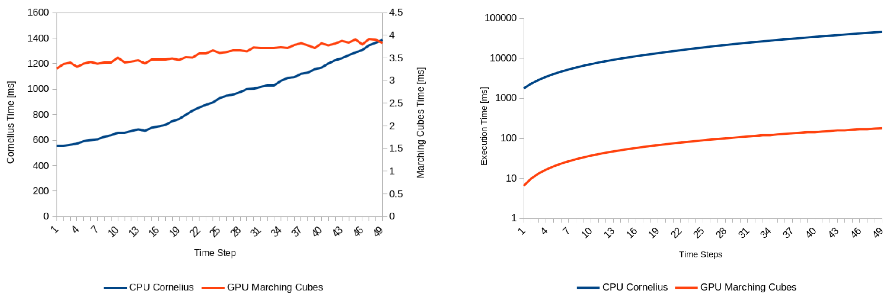
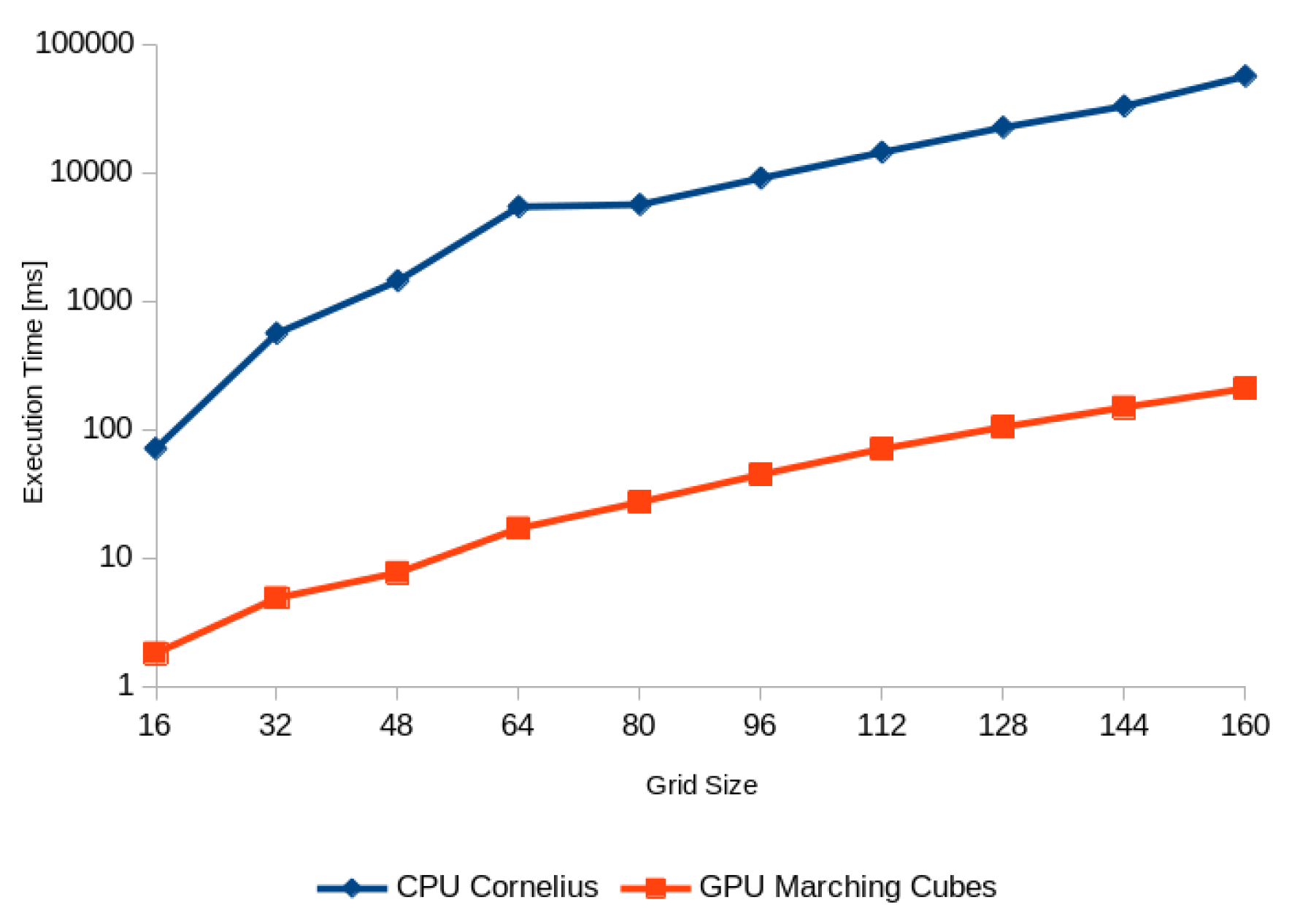
3.2. Hypersurface Extraction Methods

Table 1. Comparison of Cornelius and marching cubes methods totalled over 50 simulation steps.

Method	Time (s) (w/Copy Overhead)	Cells Intersections	Hypersurface Elements	% of Program Runtime (w/Copy Overhead)
Cornelius (single-threded)	46 (46.2)	6296765	6606727	89.1% (89.3%)
Marching cubes (parallel)	0.18	6296765	6669758	3.2%

compares single-threaded Cornelius and parallel marching cube subroutines executed over 50 numerical steps (s) of Hubble-like expansion simulated on a $128\times 128\times 128$ mesh with spatial resolution ($\Delta x,\Delta y,\Delta z$) of 0.2 fm and time resolution ($\Delta t$) of 0.06 fm. The value (energy density) used for hypersurface extraction was $ϵ=0.307$ GeV, which using Lattice-QCD (Lattice Quantum Chromodynamics) equation of state [47], stands for the temperature of 150 MeV. Figure 1 presents execution time of both methods for each of extraction step (left) and their cumulative time (right). This shows over a hundred-fold improvement in the parallel method run time, even if the data copy overhead from GPU to CPU memory necessary for Cornelius.

Additionally we observe that the execution time of the Cornelius algorithm depends heavily on the number of cells intersected by the hypersurface, which increases with each step of the expansion. With the marching cubes approach that dependence is much less pronounced, as time required for each step remains near-constant throughout the entire simulation, which indicates that most time is spent reading the state of simulation mesh from memory. That relation of execution time on mesh resolution is further demonstrated on Figure 2.

It is worth noting that our preliminary marching cubes implementation’s performance is still distant from the theoretical limit based on the number of simultaneous threads of execution on the graphics processor, which range in the thousands.

Lastly, we have verified that both methods produce a continuous freeze-out hypersurface without holes and of the same overall shape, as determined by which cells in the mesh generate hypersurface elements in each step. While those results are difficult to demonstrate, Table 1 includes the count of those cells throughout the entire simulation, which must be equal for both methods. Although both shapes are similar, Cornelius’s approximation is less complicated in terms of number of hypersurface elements.

3.3. Hydrodynamics and Kinematic Description

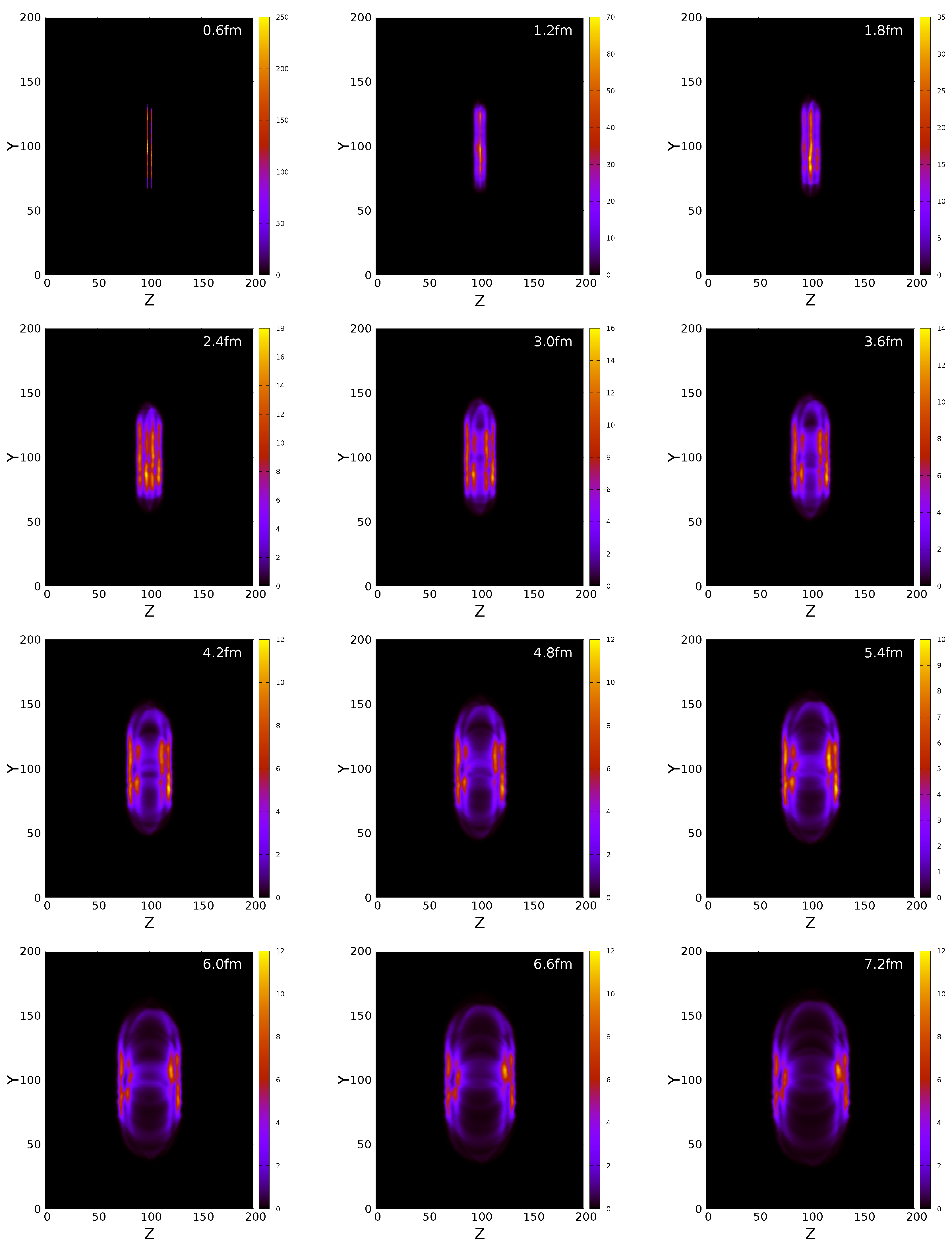
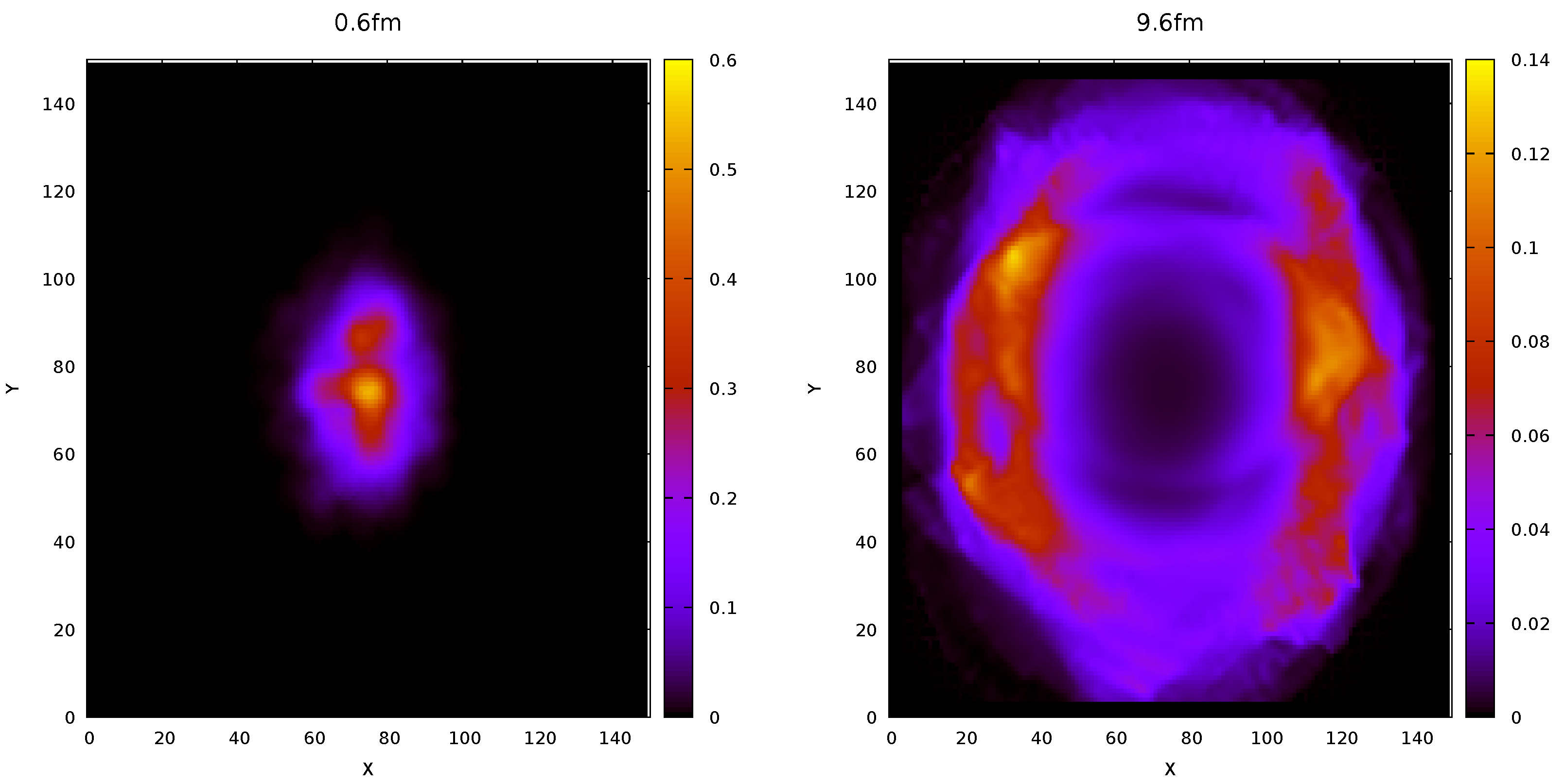
The result of the hydrodynamic simulation with the use of the developed program is the hypersurface represented as follows:

$${\overrightarrow{h}}_i=\left(t,x,y,z,{\Sigma }_t,{\Sigma }_x,{\Sigma }_y,{\Sigma }_z,V_x,V_y,V_z\right),$$

(14)

where $t,x,y,z$ are the components of the spacetime position vector, ${\Sigma }_t,{\Sigma }_x,{\Sigma }_y,{\Sigma }_z$ are the covariant normal vector ${\Sigma }_{\mu }$, and $V_x,V_y,V_z$ are the velocity. Each $i^{th}$ tuple in the Equation (14) represents of a volume element.

From the obtained hypersurface, using the “frzout” library [42], particles are sampled according to the formula of Cooper-Frye. The result of the program is a set with a list of particles. Each particle contains the following parameters:

$${\overrightarrow{p}}_i=\left(t,x,y,z,E,p_x,p_y,p_z\right),$$

(15)

where $t,x,y,z$ space-time coordinate of $i^{th}$ particle, its energy (E), and momentum components [$p_x,p_y,p_z$].

3.4. Simulation of Pb-Pb Collisions at $\sqrt{s_{NN}}=2.76$ TeV

For the presented simulations, we generate the initial conditions using UrQMD 3.4. Our initial parameters for numerical algorithm for the all simulation of Pb-Pb collisions at $\sqrt{s_{NN}}=2.76$ TeV are following: 150 numerical steps (s), $150\times 150\times 150$ mesh with spatial resolution ($\Delta x,\Delta y,\Delta z$) of 0.2 fm and time resolution ($\Delta t$) of 0.06 fm. Figure 3 shows the evolution of the hydrodynamic system in the cross-section X = 100, every 10 numerical steps. During the nucleus-nucleus collision evolution, the spatial asymmetry in coordinate space is eliminated (Figure 4). In parallel, the momentum symmetry is broken in the momentum space. There is an acceleration of matter towards the in-plane reaction plane, reflecting in the final momentum anisotropy in the $p_x{p}_y$ plane.

The crucial result of the hydrodynamic simulation is to obtain the freeze-out hypersurface, which is needed to generate particles with helps Cooper-Frye procedure. Figure 5 shows the shape of the hypersurface. In order to interpret the obtained results, we compare hypersurface from Ref. [48], which comes from hydrodynamic aHydro simulations [9] using the initial conditions Glissando generator [49]. This program implements hydrodynamics including the phenomenon of viscosity (viscosity) in the curvilinear coordinate system Milne ($\tau -x-y-\eta$). The usage of such a coordinate system facilitates the simulation of hydrodynamics but makes it difficult to observe (jets) and initial stage fluctuations phenomena. Despite the usage of different approaches, we observe that the hypersurface’s evolution in both cases is similar, and, for the “realistic” initial conditions, the hypersurface is not symmetrical and has no analytical representation.

Smooth initial conditions are possible to obtain by assuming, for example, the Gaussian distribution of matter density (taking into account Lorentzian flattening), but also by assuming a homogeneous distribution and creating a numerical grid by averaging many UrQMD events. In the case of our simulation, this is an average of 100 events (Figure 5).

Nevertheless, the homogeneous initial is a certain simplification of the dynamics of the heavy-ion collision. The developed program enables the study of initial conditions fluctuations in the simulation process, and our application introduces the algorithm for obtaining the freeze-out hypersurface.

Finally, we observe the initial conditions’ fluctuations in the figures showing the $t\left(x\right)$ hypersurface shape. Each generated hypersurface is different, which is visible in the figures below. Figure 6 shows a comparison of the hypersurface from a single UrQMD event and averaging over 10 UrQMD events.

After obtaining the hypersurface from the hydrodynamic simulation, we generate the particles using the particle generator [50]. This library is Cooper-Frye [35] sampler for relativistic heavy-ion collisions, and code is in Python language, will return a list of particles that allows preparing particle distributions.

For non-central collisions, triple differential invariant distribution of particles describe the Fourier series:

$$\begin{array}{c}E\frac{d^{3}N}{d{p}^3}=\frac{1}{2\pi }\frac{d^{2}N}{p_{T}d{p}_{T}dy}\left(1+2\sum _{n=1}^{\infty }{v}_{n}cos\left[n(\varphi -{\mathsf{\Phi }}_R)\right]\right)=\hfill \\ \hfill =\frac{1}{2\pi }\frac{d^{2}N}{p_{T}d{p}_{T}dy}\left(v_0+2v_{1}cos(\varphi -{\mathsf{\Phi }}_R)+2v_{2}cos\left[2(\varphi -{\mathsf{\Phi }}_R)\right]+...\right),\end{array}$$

(16)

where y is rapidity, $p_T$ is transverse momentum, $\varphi$ is the azimuth angle of the particle in the laboratory frame, ${\mathsf{\Phi }}_R$ is the so-called the azimuth angle of the reaction plane (RP) in the laboratory frame (various for each collision), $v_n\equiv \langle cos\left[n(\varphi -{\mathsf{\Phi }}_R)\right]\rangle$ are Fourier coefficients, $v_0$ is isotropic flow, $v_1$ is direct flow, and $v_2$ is elliptic flow. In the mid-rapidity region, the dominant effect is the elliptic flow $v_2$. However, direct flow values $v_1$ are negligible. The flow that remains for the central collisions b = 0 is the radial flow $v_0$. The direct $v_1$ and elliptic $v_2$ flows and higher harmonics $v_3-v_5$ in this case are negligible. Elliptic flow $v_2$ can measure a system’s collectivity on the non-central interactions of heavy ions, where asymmetry in coordinate space appears. Nevertheless, if there is no initial spatial asymmetry, then the elliptic flow $v_2$ is equal 0. If there is no collective behavior (no interactions), the particles is emitted as a superposition of independent sources. The particles move freely in all directions. Then, there is the isotropic azimuthal angle distribution ($v_2$ = 0) despite the interacting matter’s initial asymmetric shape. In conditions of non-central collisions, the evolution of the collective state of matter increases the pressure gradients towards the "in-plane" of the reaction plane, which increases the value of the elliptic flow $v_2$. The elliptic flow is indicative of momentum anisotropy in the $p_x{p}_y$ plane. Momentum anisotropy in $p_x{p}_y$ plane is equivalent to the anisotropy of azimuth angle.

$$\varphi =arctan\left(\frac{p_y}{p_x}\right).$$

(17)

The distribution of the azimuth angle with respect to the reaction plane shows in Figure 7 is proportional to $dN/d\varphi \sim 1+2v_{2}cos(\varphi -{\mathsf{\Phi }}_R)$. We assume that the reaction plane angle ${\mathsf{\Phi }}_R$ is equal to zero. For the mid-rapidity region, the directed flow ($v1$) is negligible. The amplitude of the azimuthal angle distribution increases with the decrease of the impact parameter ($\overrightarrow{b}$), which determines the collisions’ centrality.

The rise of elliptic flow $v_2$ with an increase in transverse momentum $p_T$ we observe in the simulations of the hydrodynamic Pb + Pb interactions at the energy of 2.76 TeV (Figure 8). The simulations have been made for the three centrality classes 0–2%, 0–5%, 30–40% of the most central collisions.

Based on the obtained results, we can conclude that our model follows the trend of experimental results and other hydrodynamic models.

4. Discussion

The hydrodynamic models in the $p_T<$1.5–2 GeV/c area describe very well data assuming that Quark-Gluon Plasma (QGP) is an ideal liquid. This type of assumption is willingly used because it facilitates the description of interactions at the microscopic (partonic) level. Hydrodynamic models describe a very strong effect of matter’s collective behavior, which considers QGP as the most ideal liquid ever observed.

Suppose we want to use hydrodynamics as a signature of a collective state of matter, where the results are comparable with the experimental data. In that case, we need to select initial geometric energy density conditions that are asymmetric in the spatial system and symmetrical in the momentum space. In hydrodynamic simulations, a transition from the asymmetric initial conditions of energy density to symmetrical distribution in the final stage of the simulation in coordinate space signalizes matter’s collective behavior.

There is also a transformation during the evolution of matter in the momentum space from symmetrical condition to asymmetrical form, reflecting the presence of a collective state of matter (Figure 4). The collectivity of the matter produced during the A + A collision and the scaling of elliptic flow $v_2$ by the number of constitutional quarks is treated as one of the main signatures of QGP formation.

5. Conclusions

We have created a simulation chain that employs programs to generate initial conditions (UrQMD). This program prepares initial conditions for hydrodynamic simulations, marching hyper-cubes algorithm or Cornelius libraries support hypersurface generation, and freeze-out library (particlization model–“frzout”) based on the Cooper-Frye method. For testing purposes, we simulate the Pb + Pb interactions for the LHC energy of 2.76 GeV. Our software will help in studying energy losses caused by the interaction of jets with bulk matter and fluctuations of the initial conditions. The advantage of using the developed model is the simulation’s computational time because the program employs GPUs and use in a Cartesian coordinate system. Our simulation procedure runs 2nd orders of magnitude faster than CPU-based programs faster with the same computational parameters. Similar gains have we observe with parallel implementation on GPU of hypersurface generation (Table 1). The program allows simulating energy changes induced by jets in bulk matter precisely using a highly resolved computational grid of up to 300${}^3$. The program may become a tool for combining hard and soft physics processes with heavy-ion interactions.

The hypersurface generated by our program is similar to that generated by other hydrodynamic codes (Figure 5). We observe an increased value of elliptic flow ($v_2$) with a decrease in the centrality of collisions which is as predicted by other hydrodynamic models (Figure 8). The two methods were implemented for freeze-out hypersurface generation of the same shape. However, it warrants further investigation whether the increased complexity of the resulting surface generated by the marching cubes algorithm has any significant negative impact on its quality or the execution time of freeze-out procedures.

In the future, we plan to perform a precise validation of the developed hydrodynamic program by comparing the results of directed, elliptic, and higher harmonic flows to experimental data and other hydrodynamic models.

References

1. Kliemant, M.; Sahoo, R.; Schuster, T.; Stock, R. Global Properties of Nucleus-Nucleus Collisions. In The Physics of the Quark-Gluon Plasma; Springer: Berlin/Heidelberg, Germany, 2010; Volume 785, pp. 23–103. [Google Scholar] [CrossRef] [Green Version]
2. Satz, H. The Thermodynamics of Quarks and Gluons. Lect. Notes Phys. 2010, 785, 1–21. [Google Scholar] [CrossRef] [Green Version]
3. Hirano, T.; van der Kolk, N.; Bilandzic, A. Hydrodynamics and Flow. Lect. Notes Phys. 2010, 785, 139–178. [Google Scholar] [CrossRef] [Green Version]
4. Schenke, B.; Jeon, S.; Gale, C. (3 + 1) D hydrodynamic simulation of relativistic heavy-ion collisions. Phys. Rev. C 2010, 82, 014903. [Google Scholar] [CrossRef]
5. Pang, L.G.; Petersen, H.; Wang, X.N. Pseudorapidity distribution and decorrelation of anisotropic flow within CLVisc hydrodynamics. Phys. Rev. C 2018, 97, 064918. [Google Scholar] [CrossRef] [Green Version]
6. Petersen, H.; Steinheimer, J.; Burau, G.; Bleicher, M.; Stöcker, H. Fully integrated transport approach to heavy ion reactions with an intermediate hydrodynamic stage. Phys. Rev. C 2008, 78, 044901. [Google Scholar] [CrossRef]
7. Gerhard, J.; Lindenstruth, V.; Bleicher, M. Relativistic hydrodynamics on graphic cards. Comput. Phys. Commun. 2013, 184, 311–319. [Google Scholar] [CrossRef] [Green Version]
8. Karpenko, I.; Huovinen, P.; Bleicher, M. A 3 + 1 dimensional viscous hydrodynamic code for relativistic heavy ion collisions. Comput. Phys. Commun. 2014, 185, 3016–3027. [Google Scholar] [CrossRef] [Green Version]
9. Alqahtani, M.; Nopoush, M.; Ryblewski, R.; Strickland, M. (3+ 1) D quasiparticle anisotropic hydrodynamics for ultrarelativistic heavy-ion collisions. Phys. Rev. Lett. 2017, 119, 042301. [Google Scholar] [CrossRef] [PubMed] [Green Version]
10. Lin, Z.W.; Ko, C.M.; Li, B.A.; Zhang, B.; Pal, S. Multiphase transport model for relativistic heavy ion collisions. Phys. Rev. C 2005, 72, 064901. [Google Scholar] [CrossRef] [Green Version]
11. Schenke, B.; Tribedy, P.; Venugopalan, R. Fluctuating Glasma initial conditions and flow in heavy ion collisions. Phys. Rev. Lett. 2012, 108, 252301. [Google Scholar] [CrossRef]
12. Moreland, J.S.; Bernhard, J.E.; Bass, S.A. Alternative ansatz to wounded nucleon and binary collision scaling in high-energy nuclear collisions. Phys. Rev. C 2015, 92, 011901. [Google Scholar] [CrossRef] [Green Version]
13. Donoho, D.L.; Grimes, C. Hessian eigenmaps: Locally linear embedding techniques for high-dimensional data. Proc. Natl. Acad. Sci. USA 2003, 100, 5591–5596. [Google Scholar] [CrossRef] [Green Version]
14. Boris, J.P.; Book, D.L. Flux-corrected transport. I. SHASTA, a fluid transport algorithm that works. J. Comput. Phys. 1973, 11, 38–69. [Google Scholar] [CrossRef]
15. Kraposhin, M.; Bovtrikova, A.; Strijhak, S. Adaptation of Kurganov-Tadmor numerical scheme for applying in combination with the PISO method in numerical simulation of flows in a wide range of Mach numbers. Procedia Comput. Sci. 2015, 66, 43–52. [Google Scholar] [CrossRef] [Green Version]
16. Huovinen, P.; Petersen, H. Particlization in hybrid models. Eur. Phys. J. A 2012, 48, 171. [Google Scholar] [CrossRef] [Green Version]
17. Weil, J.; Steinberg, V.; Staudenmaier, J.; Pang, L.; Oliinychenko, D.; Mohs, J.; Kretz, M.; Kehrenberg, T.; Goldschmidt, A.; Bäuchle, B.; et al. Particle production and equilibrium properties within a new hadron transport approach for heavy-ion collisions. Phys. Rev. C 2016, 94, 054905. [Google Scholar] [CrossRef]
18. Pierog, T.; Werner, K. EPOS model and ultra high energy cosmic rays. Nucl. Phys. B-Proc. Suppl. 2009, 196, 102–105. [Google Scholar] [CrossRef] [Green Version]
19. Bleicher, M.; Zabrodin, E.; Spieles, C.; Bass, S.A.; Ernst, C.; Soff, S.; Bravina, L.; Belkacem, M.; Weber, H.; Stöcker, H.; et al. Relativistic hadron-hadron collisions in the ultra-relativistic quantum molecular dynamics model. J. Phys. G Nucl. Part. Phys. 1999, 25, 1859. [Google Scholar] [CrossRef]
20. Miller, M.L.; Reygers, K.; Sanders, S.J.; Steinberg, P. Glauber modeling in high energy nuclear collisions. Ann. Rev. Nucl. Part. Sci. 2007, 57, 205–243. [Google Scholar] [CrossRef] [Green Version]
21. Gelis, F.; Iancu, E.; Jalilian-Marian, J.; Venugopalan, R. The Color Glass Condensate. Ann. Rev. Nucl. Part. Sci. 2010, 60, 463–489. [Google Scholar] [CrossRef] [Green Version]
22. Słodkowski, M.; Marcinkowski, P.; Gawryszewski, P.; Kikoła, D.; Porter-Sobieraj, J. Modeling of modifications induced by jets in the relativistic bulk nuclear matter. J. Phys. Conf. Ser. 2018, 1085, 052001. [Google Scholar] [CrossRef]
23. Słodkowski, M.; Gawryszewski, P.; Marcinkowski, P.; Setniewski, D.; Porter-Sobieraj, J. Simulations of Energy Losses in the Bulk Nuclear Medium Using Hydrodynamics on the Graphics Cards (GPU). Proceedings 2019, 10, 27. [Google Scholar] [CrossRef] [Green Version]
24. Marcinkowski, P.; Słodkowski, M.; Kikoła, D.; Gawryszewski, P.; Sikorski, J.; Porter-Sobieraj, J.; Zygmunt, B. Jet-induced modifications of the characteristic of the bulk nuclear matter. In Proceedings of the 15th International Conference on Strangeness in Quark Matter (SQM2015), Dubna, Russia, 6–11 July 2015; Volume 668, p. 012115. [Google Scholar] [CrossRef] [Green Version]
25. Porter-Sobieraj, J.; Słodkowski, M.; Kikoła, D.; Sikorski, J.; Aszklar, P. A MUSTA-FORCE algorithm for solving partial differential equations of relativistic hydrodynamics. Int. J. Nonlinear Sci. Numer. Simul. 2018, 19, 25–35. [Google Scholar] [CrossRef]
26. Porter-Sobieraj, J.; Cygert, S.; Kikoła, D.; Sikorski, J.; Słodkowski, M. Optimizing the computation of a parallel 3D finite difference algorithm for graphics processing units. Concurr. Comput. Pract. Exp. 2015, 27, 1591–1602. [Google Scholar] [CrossRef]
27. Nvidia, CUDA C++ Programming Guide; PG-02829-001_v11.2; Nvidia Corporation. Available online: https://docs.nvidia.com/cuda/pdf/CUDA_C_Programming_Guide.pdf (accessed on 19 March 2020).
28. Słodkowski, M.; Gawryszewski, P.; Setniewski, D. Study of the influence of initial-state fluctuations on hydrodynamic simulations. EPJ Web Conf. 2020, 245, 06005. [Google Scholar] [CrossRef]
29. Pratt, S. Accounting for backflow in hydrodynamic-Boltzmann interfaces. Phys. Rev. C 2014, 89, 024910. [Google Scholar] [CrossRef] [Green Version]
30. Adam, J.; Adamová, D.; Aggarwal, M.M.; Rinella, G.A.; Agnello, M.; Agrawal, N.; Ahammed, Z.; Ahmad, S.; Ahn, S.; Aiola, S.; et al. Anisotropic flow of charged particles in Pb-Pb collisions at s N N= 5.02 TeV. Phys. Rev. Lett. 2016, 116, 132302. [Google Scholar] [CrossRef] [PubMed] [Green Version]
31. Romatschke, P. New developments in relativistic viscous hydrodynamics. Int. J. Mod. Phys. E 2010, 19, 1–53. [Google Scholar] [CrossRef]
32. Romatschke, P.; Romatschke, U. Relativistic Fluid Dynamics in and out of Equilibrium: And Applications to Relativistic Nuclear Collisions; Cambridge Monographs on Mathematical Physics; Cambridge University Press: Cambridge, UK, 2019. [Google Scholar]
33. Burrage, K.; Butcher, J.C.; Chipman, F. An implementation of singly-implicit Runge-Kutta methods. BIT Numer. Math. 1980, 20, 326–340. [Google Scholar] [CrossRef]
34. Liu, X.D.; Osher, S.; Chan, T. Weighted essentially non-oscillatory schemes. J. Comput. Phys. 1994, 115, 200–212. [Google Scholar] [CrossRef] [Green Version]
35. Cooper, F.; Frye, G. Comment on the Single Particle Distribution in the Hydrodynamic and Statistical Thermodynamic Models of Multiparticle Production. Phys. Rev. D 1974, 10, 186. [Google Scholar] [CrossRef]
36. Huovinen, P.; Holopainen, H. Cornelius—User’s Guide. Available online: https://itp.uni-frankfurt.de/~huovinen/cornelius/guide.pdf (accessed on 19 March 2020).
37. Lorensen, W.; Cline, H. Marching Cubes: A High Resolution 3D Surface Construction Algorithm. ACM SIGGRAPH Comput. Graph. 1987, 21, 163–169. [Google Scholar] [CrossRef]
38. Nielson, G.M.; Hamann, B. The asymptotic decider: Resolving the ambiguity in Marching Cubes. IEEE Vis. 1991, 91, 83–91. [Google Scholar] [CrossRef]
39. Montani, C.; Scateni, R.; Scopigno, R. A modified look-up table for implicit disambiguation of Marching Cubes. Vis. Comput. 1994, 10, 353–355. [Google Scholar] [CrossRef]
40. Bhaniramka, P.; Wenger, R.; Crawfis, R. Isosurface construction in any dimension using convex hulls. IEEE Trans. Vis. Comput. Graph. 2004, 10, 130–141. [Google Scholar] [CrossRef]
41. Chojnacki, M.; Kisiel, A.; Florkowski, W.; Broniowski, W. THERMINATOR 2: THERMal heavy IoN generATOR 2. Comput. Phys. Commun. 2012, 183, 746–773. [Google Scholar] [CrossRef] [Green Version]
42. Bernhard, J.E. Bayesian Parameter Estimation for Relativistic Heavy-Ion Collisions. Ph.D. Thesis, Duke University, Durham, NC, USA, 2018. [Google Scholar]
43. Shu, C.W. WENO methods. Scholarpedia 2011, 6, 9709. [Google Scholar] [CrossRef]
44. Thompson, K.W. The special relativistic shock tube. J. Fluid Mech. 1986, 171, 365–375. [Google Scholar] [CrossRef]
45. Sinyukov, Y.M.; Karpenko, I.A. Ellipsoidal flows in relativistic hydrodynamics of finite systems. Acta Phys. Hung. Ser. A Heavy Ion Phys. 2006, 25, 141–147. [Google Scholar] [CrossRef] [Green Version]
46. Chojnacki, M.; Florkowski, W.; Csörgö, T. Formation of Hubble-like flow in little bangs. Phys. Rev. C 2005, 71, 044902. [Google Scholar] [CrossRef] [Green Version]
47. Bazavov, A.; Bhattacharya, T.; DeTar, C.; Ding, H.-T.; Gottlieb, S.; Gupta, R.; Hegde, P.; Heller, U.M.; Karsch, F.; Laermann, E.; et al. Equation of state in ( 2+1 )-flavor QCD. Phys. Rev. D 2014, 90, 094503. [Google Scholar] [CrossRef] [Green Version]
48. Bożek, P. Effect of bulk viscosity on interferometry correlations in ultrarelativistic heavy-ion collisions. Phys. Rev. C 2017, 95, 054909. [Google Scholar] [CrossRef] [Green Version]
49. Bożek, P.; Broniowski, W.; Rybczynski, M.; Stefanek, G. GLISSANDO 3: GLauber Initial-State Simulation AND mOre..., ver. 3. Comput. Phys. Commun. 2019, 245, 106850. [Google Scholar] [CrossRef] [Green Version]
50. Bernhard, J. Frzout -Particlization Model (Cooper-Frye Sampler) for Relativistic Heavy-Ion Collisions. Available online: http://qcd.phy.duke.edu/frzout/index.html (accessed on 19 March 2020).
Figure 1. Execution time of hypersurface extraction methods per step (left) and cumulative (right).
Symmetry 13 00507 g001
Figure 2. Influence of grid size on hypersurface extraction methods cumulative execution time.
Symmetry 13 00507 g002
Figure 3. Evolution of energy density cross-section in YZ plane in time, 0–5% most central events.
Symmetry 13 00507 g003
Figure 4. Evolution of energy density cross-section in XY plane, 30–40% most central events. (Left) panel time of the initial stage 0.6 fm. (Right) panel time of the final stage 9.6 fm.
Symmetry 13 00507 g004
Figure 5. Shapes of thefreeze-out hypersurface from the hydrodynamic simulations (Pb-Pb collisions at s N N = 2.76 TeV, 0–2% most central). Red solid line result from own Hydro on GPU and the initial conditions were generated from the UrQMD, averaging over 100 events. model. Blue dashed line result based on Ref. [48] from a Hydro3p1 and initial conditions were generated from the Glissando program.
Symmetry 13 00507 g005
Figure 6. Shapes of the freeze-out hypersurface from the hydrodynamic simulations (Pb-Pb collisions at s N N = 2.76 TeV, 0–2% most central). Red solid line represents a result from our hydrodynamic model on GPU using UrQMD model as an initial conditions generator. Left panel–averaging over 10 UrQMD events, right panel–single UrQMD event.
Symmetry 13 00507 g006
Figure 7. Distribution of the azimuth angle. Azimuth angle distribution as a result of the hydrodynamic simulation on the GPU for 2000 UrQMD events. Green dashed line is 0–2%, blue dashed line is 0–5%, and red solid line is 30–40% most central events.
Symmetry 13 00507 g007
Figure 8. Elliptic flow ( v 2 ) as a function transverse momentum p T . Green dashed line is 0–2%, blue dashed line is 0–5%, and red solid line is 30–40% most central events (2000 events for each case).
Symmetry 13 00507 g008