A Mean Extragradient Method for Solving Variational Inequalities

Abstract

We propose a modified extragradient method for solving the variational inequality problem in a Hilbert space. The method is a combination of the well-known subgradient extragradient with the Mann’s mean value method in which the updated iterate is picked in the convex hull of all previous iterates. We show weak convergence of the mean value iterate to a solution of the variational inequality problem, provided that a condition on the corresponding averaging matrix is fulfilled. Some numerical experiments are given to show the effectiveness of the obtained theoretical result.

1. Introduction

Let $\mathcal{H}$ be a real Hilbert space with an inner product $\langle ·,·\rangle$ and the associated norm $\Vert ·\Vert$. Let C be a nonempty closed convex subset of $\mathcal{H}$, and let $F:\mathcal{H}\to \mathcal{H}$ be a monotone operator defined by

$$〈x-y,F\left(x\right)-F\left(y\right)〉\ge 0,$$

for all $x,y\in \mathcal{H}$, and a L-Lipschitz continuous operator defined by

$$\parallel F\left(x\right)-F\left(y\right)\parallel \le L\parallel x-y\parallel ,$$

for all $x,y\in \mathcal{H}$. The (Stampacchia) variational inequality problem is to find a point $x^{*}\in C$ such that

$$\begin{array}{c}\hfill \langle F\left(x^{*}\right),z-x^{*}\rangle \ge 0\mathrm{for}\mathrm{all}z\in C.\end{array}$$

(1)

We will denote the solution set of the considered variational inequality by $\mathrm{VIP}(F,C)$ and assume that it is nonempty. Since $\mathrm{VIP}(F,C)$ has been utilized for modeling many mathematical and practical situations (see [1] for insight discussions), many iterative methods have been proposed for solving it. The classical method is due to Goldstein [2] which can be read in the form: for a given $x_1\in \mathcal{H}$, calculate

$$\begin{array}{c}\hfill x_{k+1}:=P_C(x_k-\tau F\left(x_k\right)),k\in \mathbb{N},\end{array}$$

(2)

where $\tau >0$ is a step-size parameter and $P_C$ is the metric projection onto C. By assuming that F is $\eta$-strongly monotone and L-Lipschitz continuous and $\tau \in (0,2\eta /L^2)$, it has been proved that the sequence generated by (2) converges strongly to the unique solution of $\mathrm{VIP}(F,C)$.

As the convergence of the iterative scheme in (2) needs to use the strong monotonicity of F which is quite restricted, in 1976, Korpelevich [3] proposed the so-called extragradient method (in short, EM), which is defined by the following form: for a given $x_1\in \mathcal{H}$, calculate

$$\begin{array}{c}\hfill \left\{\begin{array}{cc}\hfill y_k& :=P_C(x_k-\tau F\left(x_k\right)),\hfill \\ \hfill x_{n+1}& :=P_C(x_k-\tau F\left(y_k\right)),k\in \mathbb{N}.\hfill \end{array}\right.\end{array}$$

(3)

In the setting of a finite dimensional space, it has been proved that the sequence generated by EM (3) converges to a solution of $\mathrm{VIP}(F,C)$ governed by Lipschitz continuity and monotonicity of F. From such starting point, several variants of Korpelevich’s EM have been investigated, for instance [4,5,6,7,8,9] and references there cited in. Especially, we only underline here the work of Censor, Gibali and Reich [10]. As one can see from the above scheme, EM requires the performing of two metric projections in each iteration. For this reason, EM will be suitable for the case when the constrained set C is simple enough so that the metric projection $P_C$ onto C has a closed-form expression, otherwise one needs to solve a hidden minimization sub-problem. To avoid this situation, Censor, Gibali and Reich proposed the so-called subgradient–extragradient method (SEM), which requires only one metric projection onto C for updating $y_k$, meanwhile, another one is replaced by the metric projection onto a half-space containing C for updating the next iterate $x_{k+1}$. The method essentially has the form:

$$\begin{array}{c}\hfill \left\{\begin{array}{cc}\hfill y_k& :=P_C(x_k-\tau F\left(x_k\right)),\hfill \\ \hfill x_{n+1}& :=P_{T_k}(x_k-\tau F\left(y_k\right)),k\in \mathbb{N},\hfill \end{array}\right.\end{array}$$

(4)

where

$$T_k:=\{w\in \mathcal{H}:\langle (x_k-\tau F\left(x_k\right))-y_k,w-y_k\rangle \le 0\}.$$

It is worth noting that the closed-form expression of $P_{T_k}$ is explicitly given in the literature (see the Formula (7) for further details). The weak convergence result is also given in the paper [10]. Several variants of SEM have been investigated, see for instance [11,12,13,14,15,16]. Note that, even if SEM has the advantage of reducing the performance of the metric projection onto C when performing $x_{k+1}$, there still is the metric projection when evaluating $y_k$, in this situation the inner-loop iteration remains when the constrained set C is not simple enough, for example, the intersection of a finite number of nonempty closed convex simple sets.

On the other hand, let us move to another aspect of the nonlinear problem. Let $T:\mathcal{H}\to \mathcal{H}$ be a nonlinear operator, the celebrate fixed-point problem is to find $x^{*}\in FixT:=\{x\in \mathcal{H}:x=Tx\}\ne \varnothing$. In order to solve this problem, we recall the classical Picard’s iteration which updates the next iterate $x_{k+1}$ by using the information of the current iterate $x_k$, that is

$$x_{k+1}:=T{x}_k,k\in \mathbb{N}.$$

This kind of method is known as the memoryless scheme, and it is well-known in the literature that the sequence generated by Picard’s iterative method may fail to converge to a point in $FixT$. In 1953, Mann [17] proposed a modified version of Picard’s iteration as

$$x_{k+1}:=T{\overline{x}}_k,k\in \mathbb{N},$$

where ${\overline{x}}_k$ denotes a convex combination of the iterates ${\left\{x_j\right\}}_{j=1}^k$, or in another word, ${\overline{x}}_k$ is a point in the convex hull of all previous iterates. This method is known as Mann’s mean value iteration. The advantage of Mann’s mean value iteration is underlined for avoiding some numerical desirable situations, for instance, the generated sequence may have zig–zag or spiral behavior around the solution set, see [18] for more insight discussion. Some works based on the idea of Mann’s mean value iteration have been investigated, for instance [18,19].

In this work, we present an iterative method by utilizing the ideas of the celebrated SEM together with Mann’s mean value iteration for solving $\mathrm{VIP}(F,C)$ governed by monotone and Lipschitz continuous operator. We show that the sequence generated by the proposed method converges weakly to a solution of $\mathrm{VIP}(F,C)$. To demonstrate the numerical behavior of the proposed method, we consider the constrained minimization problem in which the constrained set is given by the intersection of a finite family nonempty closed convex simple sets. We present numerical experiments which show that, under some suitable parameters, the proposed method outperforms the existing one.

2. Preliminaries

For convenience, we present here some notations which are used throughout the paper. For more details, the reader may consult the reference books [20,21].

We denote the strong convergence and weak convergence of a sequence ${\left\{x_k\right\}}_{k=1}^{\infty }$ to $x\in \mathcal{H}$ by $x_k\to x$ and $x_k\rightharpoonup x$, respectively. We denote the identity operator on $\mathcal{H}$ by $Id$.

Let C be a nonempty, closed, and convex subset of $\mathcal{H}$. For each point $x\in \mathcal{H},$ there exists a unique nearest point in C, denoted by $P_C\left(x\right)$, that is,

$$\begin{array}{c}\hfill \parallel x-P_C\left(x\right)\parallel =\underset{y\in C}{inf}\parallel x-y\parallel .\end{array}$$

(5)

The mapping $P_C:\mathcal{H}\to C$ is called the metric projection of $\mathcal{H}$ onto C. Note that $P_C$ is a nonexpansive mapping of $\mathcal{H}$ onto C, i.e.,

$$\begin{array}{c}\hfill \parallel P_C\left(x\right)-P_C\left(y\right)\parallel \le \parallel x-y\parallel ,\forall x,y\in \mathcal{H}.\end{array}$$

Moreover, the metric projection $P_C$ satisfies the variational property:

$$\langle x-P_C\left(x\right),P_C\left(x\right)-y\rangle \ge 0,\forall x\in \mathcal{H},y\in C.$$

(6)

Let $a\in \mathcal{H}\setminus \left\{0\right\}$ and $\beta \in \mathbb{R}$, we define the hyperplane in $\mathcal{H}$ by

$$\begin{array}{c}\hfill H(a;\beta ):=\{x\in \mathcal{H}:\langle a,x\rangle =\beta \},\end{array}$$

and the half-space in $\mathcal{H}$ by

$$\begin{array}{c}\hfill H_{\le }(a;\beta ):=\{x\in \mathcal{H}:\langle a,x\rangle \le \beta \}.\end{array}$$

It is clear that both hyperplane and half-space are closed and convex sets. Moreover, it is important to note that the metric projection onto the half-space $H_{\le }(a;\beta )$ can be done explicitly as the following formula:

$$\begin{array}{c}\hfill P_{H_{\le }(a;\beta )}\left(x\right):=\left\{\begin{array}{cc}x-\frac{〈a,x〉-\beta }{{\parallel a\parallel }^2}a,\hfill & \mathrm{if}\langle a,x\rangle >\beta ,\hfill \\ x,\hfill & \mathrm{if}\langle a,x\rangle \le \beta .\hfill \end{array}\right.\end{array}$$

(7)

For a point $x\in \mathcal{H}$ and a nonempty closed convex $C\subset \mathcal{H}$, we say that a point $z\in \mathcal{H}$ separates C from x if,

$$\begin{array}{c}\hfill \langle x-z,z-y\rangle \ge 0,\forall y\in C.\end{array}$$

We say that an operator $T:C\to \mathcal{H}$ is a separator of C if the point $Tx$ separates C from a point x for all $x\in \mathcal{H}$. It is clear from the relation (6) that the projection $P_C$ is a separator of C. It is worth noting that for any $x\notin C$, the hyperplane $H(x-P_C\left(x\right);\langle P_C\left(x\right),x-P_C\left(x\right)\rangle )$ cuts the space $\mathcal{H}$ into two half-spaces. One space contains the element x while the other one contains the subset C. We also know that

$$C\subset H_{\le }(x-P_C\left(x\right);\langle P_C\left(x\right),x-P_C\left(x\right)\rangle ),$$

and the hyperplane $H_{\le }(x-P_C\left(x\right);\langle P_C\left(x\right),x-P_C\left(x\right)\rangle )$ is a supporting hyperplane to C at the point $P_C\left(x\right)$.

Let $A:\mathcal{H}\to 2^{\mathcal{H}}$ be a set-valued operator. We denote its graph by

$$\mathrm{Gr}\left(A\right):=\left\{\right(x,u)\in \mathcal{H}\times \mathcal{H}:u\in Ax\}.$$

We denote the set of all zeros of A by

$$A^{-1}\left(0\right):=\{x\in \mathcal{H}:0\in A\left(x\right)\}.$$

The operator A is said to be monotone if

$$\langle x-y,u-v\rangle \ge 0,$$

for all $(x,u),(y,v)\in \mathrm{Gr}\left(A\right),$ and it is called maximally monotone if its graph is not properly contained in the graph of any other monotone operator. Note that if A is maximally monotone, then $A^{-1}\left(0\right)$ is a convex and closed set.

Let $C\subset \mathcal{H}$ be a nonempty closed convex set. We denote by $N_C\left(x\right)$ the normal cone to C at $x\in C$, i.e.,

$$\begin{array}{c}\hfill N_C\left(x\right):=\{y\in \mathcal{H}:\langle y,z-x\rangle \le 0,\forall z\in C\}.\end{array}$$

Let $F:\mathcal{H}\to \mathcal{H}$ be a monotone continuous operator and C be a nonempty closed convex subset of $\mathcal{H}$. Define the operator $A:\mathcal{H}\to 2^{\mathcal{H}}$ by

$$\begin{array}{c}\hfill A\left(x\right):=\left\{\begin{array}{cc}F\left(x\right)+N_C\left(x\right),\hfill & \mathrm{for}x\in C,\hfill \\ \varnothing ,\hfill & \mathrm{for}x\notin C.\hfill \end{array}\right.\end{array}$$

Then, we have A is a maximally monotone operator, and the following important property holds:

$$\mathrm{VIP}(F,C)=A^{-1}\left(0\right).$$

3. Mann’s Type Mean Extragradient Algorithm

In this section, we present a mean extragradient algorithm for solving the considered variational inequality problem.

We start with recalling the so-called averaging matrix as follows. An infinite lower triangular row matrix ${\left[{\alpha }_{k,j}\right]}_{k,j=1}^{\infty }$ is said to be averaging if the following conditions are satisfied:

(A1)

for all $k,j\ge 1$, ${\alpha }_{k,j}\ge 0$;

(A2)

for all $k\ge 1$, if $j>k$, then ${\alpha }_{k,j}=0$;

(A3)

for all $k\ge 1$, ${\sum }_{j=1}^k{\alpha }_{k,j}=1$;

(A4)

for all $j\ge 1$, ${lim}_{k\to +\infty }{\alpha }_{k,j}=0$.

For a sequence ${\left\{x_k\right\}}_{k=1}^{\infty }\subset \mathcal{H}$ and an averaging matrix ${\left[{\alpha }_{k,j}\right]}_{k,j=1}^{\infty }$, we denote the mean iterate by

$${\overline{x}}_k=\sum _{j=1}^k{\alpha }_{k,j}{x}_j,$$

for all $k\ge 1$.

Now, we are in position to state the Mann mean extragradient method (Mann-MEM) as follows Algorithm 1.

Algorithm 1: Mann’s type mean extragradient method (Mann-MEM).

Initialization: Select a point $x_1\in \mathcal{H}$, a parameter $\tau >0$ and an averaging matrix ${\left[{\alpha }_{k,j}\right]}_{k,j=1}^{\infty }$.   Step 1: Given a current iterate $x_k\in \mathcal{H}$, compute the mean iterate $${\overline{x}}_k=\sum _{j=1}^k{\alpha }_{k,j}{x}_j.$$   Compute $$y_k=P_C({\overline{x}}_k-\tau F\left({\overline{x}}_k\right)).$$   Step 2: If $y_k={\overline{x}}_k$, then ${\overline{x}}_k\in \mathrm{VIP}(F,C)$ and STOP.   If not, construct the half-space $T_k$ defined by $$T_k:=\{w\in \mathcal{H}:\langle ({\overline{x}}_k-\tau F\left({\overline{x}}_k\right))-y_k,w-y_k\rangle \le 0\},$$   and calculate the next iterate $$x_{k+1}=P_{T_k}({\overline{x}}_k-\tau F\left(y_k\right)).$$   Update $k=k+1$ and go to Step 1.

Remark 1.

In the case that the averaging matrix ${\left[{\alpha }_{k,j}\right]}_{k,j=1}^{\infty }$ is the identity matrix, then Mean-MEM is reduced to the classical subgradient extragradient method proposed by Censor et al. [10] Algorithm 4.1.

The following proposition confirms us a stopping criterion of Mann-MEM on Step 2.

Proposition 1.

Let ${\left\{{\overline{x}}_k\right\}}_{k=1}^{\infty }$ and ${\left\{y_k\right\}}_{k=1}^{\infty }$ be sequences generated by $\mathrm{Mann}-\mathrm{MEM}$. If there is $k_0\in \mathbb{N}$ such that $y_{k_0}={\overline{x}}_{k_0}$, then ${\overline{x}}_{k_0}\in \mathrm{VIP}(F,C)$.

Proof. 

Let $k_0\in \mathbb{N}$ be such that $y_{k_0}={\overline{x}}_{k_0}$. Then, by the definition of $y_k$, we have ${\overline{x}}_{k_0}=y_{k_0}=P_C({\overline{x}}_{k_0}-\tau F\left({\overline{x}}_{k_0}\right))$, which yields that ${\overline{x}}_{k_0}\in C$. For every $z\in C$, we have from the inequality (6) that

$$〈z-{\overline{x}}_{k_0},{\overline{x}}_{k_0}-\tau F\left({\overline{x}}_{k_0}\right)-{\overline{x}}_{k_0}〉\le 0,$$

and then

$$〈z-{\overline{x}}_{k_0},F\left({\overline{x}}_{k_0}\right)〉\ge 0,$$

which holds by the fact that $\tau >0$. Hence, we conclude that ${\overline{x}}_{k_0}\in \mathrm{VIP}(F,C)$ as required. □

According to Proposition 1, for the rest of our convergence analysis, we may assume throughout this section that Mann-MEM does not terminate after a finite number of iterations, that is, we assume that $y_k\ne {\overline{x}}_k$ for all $k\ge 1$.

The following technical lemma is a key tool in order to prove the convergence result of a sequence generated by $\mathrm{Mann}-\mathrm{MEM}$.

Lemma 1.

Let ${\left\{x_k\right\}}_{k=1}^{\infty }$ be a sequence generated by $\mathrm{Mann}-\mathrm{MEM}$. For every $k\ge 1$ and $u\in \mathrm{VIP}(F,C)$, it holds that

$$\parallel x_{k+1}{-u\parallel }^2\le \parallel {\overline{x}}_k{-u\parallel }^2-(1-{\tau }^2{L}^2)\parallel {\overline{x}}_k-y_k{\parallel }^2\le \sum _{j=1}^k{\alpha }_{k,j}\parallel x_j{-u\parallel }^2-(1-{\tau }^2{L}^2){\parallel {\overline{x}}_k-y_k\parallel }^2.$$

Proof. 

Let $k\ge 1$ and $u\in \mathrm{VIP}(F,C)$ be fixed. Since F is monotone, we note that

$$\langle F\left(y_k\right)-F\left(u\right),y_k-u\rangle \ge 0,$$

which implies that

$$\begin{array}{c}\hfill \langle F\left(y_k\right),y_k-u\rangle \ge \langle F\left(u\right),y_k-u\rangle \ge 0,\end{array}$$

where the second inequality holds true by the fact that $y_k\in C$ and $u\in \mathrm{VIP}(F,C)$. Thus, we also have

$$\begin{array}{c}\hfill \langle F\left(y_k\right),x_{k+1}-u\rangle \ge \langle F\left(y_k\right),x_{k+1}-y_k\rangle .\end{array}$$

(8)

Now, invoking the definition of $T_k$, we note that

$$\langle x_{k+1}-y_k,({\overline{x}}_k-\tau F\left({\overline{x}}_k\right))-y_k\rangle \le 0.$$

and, it follows that

$$\begin{array}{cc}\hfill \langle x_{k+1}-y_k,{\overline{x}}_k-\tau F\left(y_k\right)-y_k\rangle =& \langle x_{k+1}-y_k,{\overline{x}}_k-\tau F\left({\overline{x}}_k\right)-y_k\rangle \hfill \\ \hfill & +\langle x_{k+1}-y_k,-\tau (F\left(y_k\right)-F\left({\overline{x}}_k\right))\rangle \hfill \\ \hfill \le & \tau \langle x_{k+1}-y_k,F\left({\overline{x}}_k\right)-F\left(y_k\right)\rangle .\hfill \end{array}$$

(9)

Denoting $z_k:={\overline{x}}_k-\tau F\left(y_k\right)$, we note that

$$\begin{array}{ccc}\hfill \parallel x_{k+1}{-u\parallel }^2& =& \parallel P_{T_k}\left(z_k\right){-u\parallel }^2\hfill \\ & =& \parallel P_{T_k}\left(z_k\right)-z_k+z_k{-u\parallel }^2\hfill \\ & =& \parallel P_{T_k}\left(z_k\right)-z_k{\parallel }^2+{\parallel z_k-u\parallel }^2+2\langle P_{T_k}\left(z_k\right)-z_k,z_k-u\rangle .\hfill \end{array}$$

(10)

Note that, it follows from the variational property of $P_{T_k}$ that

$$\begin{array}{ccc}\hfill 0& \ge & 2\langle z_k-P_{T_k}\left(z_k\right),u-P_{T_k}\left(z_k\right)\rangle \hfill \\ & =& 2\parallel z_k-P_{T_k}\left(z_k\right){\parallel }^2+2\langle P_{T_k}\left(z_k\right)-z_k,z_k-u\rangle ,\hfill \end{array}$$

and which yields that

$$\begin{array}{c}\hfill \parallel z_k-P_{T_k}\left(z_k\right){\parallel }^2+2\langle P_{T_k}\left(z_k\right)-z_k,z_k-u\rangle \le -{\parallel z_k-P_{T_k}\left(z_k\right)\parallel }^2.\end{array}$$

(11)

By substituting (11) in (10), we obtain

$$\begin{array}{ccc}\hfill \parallel x_{k+1}{-u\parallel }^2& \le & \parallel z_k{-u\parallel }^2-{\parallel z_k-P_{T_k}\left(z_k\right)\parallel }^2\hfill \\ & =& \parallel {\overline{x}}_k-\tau F\left(y_k\right){-u\parallel }^2-{\parallel {\overline{x}}_k-\tau F\left(y_k\right)-x_{k+1}\parallel }^2\hfill \\ & =& \parallel {\overline{x}}_k{-u\parallel }^2+{\tau }^2{\parallel F\left(y_k\right)\parallel }^2-2\tau \langle F\left(y_k\right),{\overline{x}}_k-u\rangle \hfill \\ & & -\parallel {\overline{x}}_k-x_{k+1}{\parallel }^2-{\tau }^2{\parallel F\left(y_k\right)\parallel }^2+2\tau \langle F\left(y_k\right),{\overline{x}}_k-x_{k+1}\rangle \hfill \\ & =& \parallel {\overline{x}}_k{-u\parallel }^2-{\parallel {\overline{x}}_k-x_{k+1}\parallel }^2+2\tau \langle F\left(y_k\right),u-x_{k+1}\rangle .\hfill \end{array}$$

Thus, from above inequality and by using (8), (9), we have

$$\begin{array}{ccc}\hfill \parallel x_{k+1}{-u\parallel }^2& \le & \parallel {\overline{x}}_k{-u\parallel }^2-{\parallel {\overline{x}}_k-x_{k+1}\parallel }^2+2\tau \langle F\left(y_k\right),y_k-x_{k+1}\rangle \hfill \\ & \le & \parallel {\overline{x}}_k{-u\parallel }^2-{\parallel {\overline{x}}_k-y_k+y_k-x_{k+1}\parallel }^2+2\tau \langle F\left(y_k\right),y_k-x_{k+1}\rangle \hfill \\ & =& \parallel {\overline{x}}_k{-u\parallel }^2-\parallel {\overline{x}}_k-y_k{\parallel }^2-{\parallel y_k-x_{k+1}\parallel }^2-2\langle {\overline{x}}_k-y_k,y_k-x_{k+1}\rangle \hfill \\ & & +2\tau \langle F\left(y_k\right),y_k-x_{k+1}\rangle \hfill \\ & =& \parallel {\overline{x}}_k{-u\parallel }^2-\parallel {\overline{x}}_k-y_k{\parallel }^2-{\parallel y_k-x_{k+1}\parallel }^2-2\langle y_k-x_{k+1},{\overline{x}}_k-y_k-\tau F\left(y_k\right)\rangle \hfill \\ & \le & \parallel {\overline{x}}_k{-u\parallel }^2-\parallel {\overline{x}}_k-y_k{\parallel }^2-{\parallel y_k-x_{k+1}\parallel }^2+2\tau \langle y_k-x_{k+1},F\left({\overline{x}}_k\right)-F\left(y_k\right)\rangle \hfill \\ & \le & \parallel {\overline{x}}_k{-u\parallel }^2-\parallel {\overline{x}}_k-y_k{\parallel }^2-\parallel y_k-x_{k+1}{\parallel }^2+2\tau \parallel y_k-x_{k+1}\parallel \parallel F\left({\overline{x}}_k\right)-F\left(y_k\right)\parallel .\hfill \\ \hfill \end{array}$$

(12)

By using the L-Lipschitz continuity of F and the fact that $2ab\le a^2+b^2$ for all $a,b\in \mathbb{R}$, we have

$$\begin{array}{ccc}\hfill \parallel x_{k+1}{-u\parallel }^2& \le & \parallel {\overline{x}}_k{-u\parallel }^2-\parallel {\overline{x}}_k-y_k{\parallel }^2-{\parallel y_k-x_{k+1}\parallel }^2\hfill \\ & & +2\tau L\parallel y_k-x_{k+1}\parallel \parallel {\overline{x}}_k-y_k\parallel \hfill \\ & \le & \parallel {\overline{x}}_k{-u\parallel }^2-\parallel {\overline{x}}_k-y_k{\parallel }^2-{\parallel y_k-x_{k+1}\parallel }^2\hfill \\ & & +{\tau }^2{L}^2\parallel {\overline{x}}_k-y_k{\parallel }^2+{\parallel y_k-x_{k+1}\parallel }^2\hfill \\ & =& \parallel {\overline{x}}_k{-u\parallel }^2-(1-{\tau }^2{L}^2){\parallel {\overline{x}}_k-y_k\parallel }^2.\hfill \end{array}$$

Finally, by using the assumption that ${\left[{\alpha }_{k,j}\right]}_{k,j=1}^{\infty }$ is an averaging matrix, and the convexity of ${\parallel ·\parallel }^2$, we have

$$\begin{array}{ccc}\hfill \parallel x_{k+1}{-u\parallel }^2& \le & \parallel {\overline{x}}_k{-u\parallel }^2-(1-{\tau }^2{L}^2){\parallel {\overline{x}}_k-y_k\parallel }^2\hfill \\ & =& {∥\sum _{j=1}^k{\alpha }_{k,j}{x}_j-\sum _{j=1}^k{\alpha }_{k,j}u∥}^2-(1-{\tau }^2{L}^2){\parallel {\overline{x}}_k-y_k\parallel }^2\hfill \\ & =& {∥\sum _{j=1}^k{\alpha }_{k,j}(x_j-u)∥}^2-(1-{\tau }^2{L}^2){\parallel {\overline{x}}_k-y_k\parallel }^2\hfill \\ & \le & \sum _{j=1}^k{\alpha }_{k,j}\parallel x_j{-u\parallel }^2-(1-{\tau }^2{L}^2){\parallel {\overline{x}}_k-y_k\parallel }^2,\hfill \end{array}$$

and the proof is completed. □

Next, we recall the following concept which plays a crucial role in the convergence analysis of our work. The following proposition is very useful in our convergence proof, and it is due to [22] (Section 3.5, Theorem 4).

Proposition 2.

Let ${\left\{{\phi }_k\right\}}_{k=1}^{\infty }$ be a real sequence, $r\in \mathbb{R}$, and ${\left[{\alpha }_{k,j}\right]}_{k,j=1}^{\infty }$ be an averaging matrix. If ${\phi }_k\to r$, then ${\overline{\phi }}_k:={\sum }_{j=1}^k{\alpha }_{k,j}{\phi }_j\to r$.

An averaging matrix ${\left[{\alpha }_{k,j}\right]}_{k,j=1}^{\infty }$ is said to be M-concentrating [18] if for every nonnegative real sequences ${\left\{{\phi }_k\right\}}_{k=1}^{\infty }$, and ${\left\{\epsilon \right\}}_{k=1}^{\infty }$ such that ${\sum }_{k=1}^{\infty }{\epsilon }_k<+\infty$ and it holds that

$$\begin{array}{c}\hfill {\phi }_{k+1}\le {\overline{\phi }}_k+{\epsilon }_k,\end{array}$$

(13)

where ${\overline{\phi }}_k:={\sum }_{j=1}^k{\alpha }_{k,j}{\phi }_j$, for all $k\ge 1$, we have the limit ${lim}_{k\to \infty }{\phi }_k$ exists.

Note that in view of Lemma 1, if we add an additional prior criterion on $\tau$ so that the term $(1-{\tau }^2{L}^2){\parallel {\overline{x}}_k-y_k\parallel }^2$ of the right-hand side is nonpositive, together with the assumtion that the averaging matrix ${\left[{\alpha }_{k,j}\right]}_{k,j=1}^{\infty }$ is M-concentrating, it will yield the convergence of the sequence $\{\parallel x_k-u{{\parallel }^2\}}_{k=1}^{\infty }$. Now, we are in a position to formally state the convergence analysis of Mann-MEM.

Theorem 1.

Assume that the averaging matrix ${\left[{\alpha }_{k,j}\right]}_{k,j=1}^{\infty }$ is M-concentrating and $\tau \in (0,1/L)$. Then any sequence ${\left\{{\overline{x}}_k\right\}}_{k=1}^{\infty }$ generated by $\mathrm{Mann}-\mathrm{MEM}$ converges weakly to a solution in $\mathrm{VIP}(F,C)$.

Proof. 

Let $k\ge 1$ and $u\in \mathrm{VIP}(F,C)$ be fixed. Now, we note from Lemma 1 that

$$\parallel x_{k+1}{-u\parallel }^2\le \sum _{j=1}^k{\alpha }_{k,j}\parallel x_j{-u\parallel }^2-(1-{\tau }^2{L}^2){\parallel {\overline{x}}_k-y_k\parallel }^2.$$

(14)

Since $\tau \in (0,1/L)$, we have

$$\begin{array}{c}\hfill 0<1-{\tau }^2{L}^2<1,\end{array}$$

(15)

and then the inequality (14) can be written as

$$\parallel x_{k+1}{-u\parallel }^2\le \sum _{j=1}^k{\alpha }_{k,j}{\parallel x_j-u\parallel }^2.$$

In view of $\phi :=\parallel x_k{-u\parallel }^2$ and ${\epsilon }_k:=0$ for every $k\ge 1$ in (13), and by using the assumption that the averaging matrix ${\left[{\alpha }_{k,j}\right]}_{k,j=1}^{\infty }$ is M-concentrating, we obtain that ${lim}_{k\to \infty }\left|\right|x_k{-u\parallel }^2$ exists, say $r\left(u\right)\in \mathbb{R}$. Invoking Lemma 2, we have ${lim}_{k\to \infty }{\sum }_{j=1}^k{\alpha }_{k,j}{\parallel x_j-u\parallel }^2$ exists with the same limit $r\left(u\right)$, and subsequently, it follows from these together with (14) and $0<1-{\tau }^2{L}^2<1$ that

$$\begin{array}{c}\hfill \underset{k\to \infty }{lim}\parallel {\overline{x}}_k-y_k\parallel =0.\end{array}$$

(16)

Moreover, we note that from Lemma 1 again that

$$\parallel x_{k+1}{-u\parallel }^2\le \parallel {\overline{x}}_k{-u\parallel }^2\le \sum _{j=1}^k{\alpha }_{k,j}{\parallel x_j-u\parallel }^2,$$

we also have ${lim}_{k\to \infty }{\parallel {\overline{x}}_k-u\parallel }^2=r\left(u\right)$.

Since the sequence ${\left\{{\overline{x}}_k\right\}}_{k=1}^{\infty }$ is bounded, there are a weak cluster point $x^{\prime }\in \mathcal{H}$ and a subset ${\left\{{\overline{x}}_{k_i}\right\}}_{i=1}^{\infty }$ such that ${\overline{x}}_{k_i}\rightharpoonup x^{\prime }$. Thus, it follows from (16) that $y_{k_i}\rightharpoonup x^{\prime }$.

Now, let us define the operator $A:\mathcal{H}\to 2^{\mathcal{H}}$ by

$$\begin{array}{c}\hfill A\left(v\right):=\left\{\begin{array}{cc}F\left(v\right)+N_C\left(v\right),\hfill & \mathrm{for}v\in C,\hfill \\ \varnothing ,\hfill & \mathrm{otherwise}.\hfill \end{array}\right.\end{array}$$

Then, we know that A is a maximally monotone operator and $A^{-1}\left(0\right)=\mathrm{VIP}(F,C)$. Further, for $(v,w)\in G\left(A\right)$, that is $w\in A\left(v\right)=F\left(v\right)+N_C\left(v\right)$, we have $w-F\left(v\right)\in N_C\left(v\right)$ which means that

$$\begin{array}{c}\hfill \langle w-F\left(v\right),v-y\rangle \ge 0 \forall y\in C.\end{array}$$

(17)

Thus, by the variational property of $y_k$, we have

$$\langle {\overline{x}}_k-\tau F\left({\overline{x}}_k\right)-y_k,y_k-v\rangle \ge 0,$$

that is,

$$\begin{array}{c}\hfill 〈\left(\frac{y_k-{\overline{x}}_k}{\tau }\right)+F\left({\overline{x}}_k\right),v-y_k〉\ge 0,\end{array}$$

(18)

for all $k\ge 1$. Hence, by using (17) and (18) and replacing y by $y_{k_i}$ and $y_k$ by $y_{k_i}$, respectively, we have

$$\begin{array}{ccc}\hfill \langle w,v-y_{k_i}\rangle & \ge & \langle F\left(v\right),v-y_{k_i}\rangle \hfill \\ & \ge & \langle F\left(v\right),v-y_{k_i}\rangle -〈\left(\frac{y_{k_i}-{\overline{x}}_{k_i}}{\tau }\right)+F\left({\overline{x}}_{k_i}\right),v-y_{k_i}〉\hfill \\ & =& \langle F\left(v\right)-F\left(y_{k_i}\right),v-y_{k_i}\rangle +\langle F\left(y_{k_i}\right)-F\left({\overline{x}}_{k_i}\right),v-y_{k_i}\rangle \hfill \\ & & -〈\left(\frac{y_{k_i}-{\overline{x}}_{k_i}}{\tau }\right),v-y_{k_i}〉\hfill \end{array}$$

Taking the limit as $i\to \infty$, we obtain

$$\langle w,v-x^{\prime }\rangle \ge 0.$$

Now, since A is a maximally monotone operator, we obtain that $x^{\prime }\in A^{-1}\left(0\right)=\mathrm{VIP}(F,C).$

Next, we show that the whole sequence converges weakly to $x^{\prime }$. Assume that there is a subsequence ${\left\{{\overline{x}}^j\right\}}_{j=1}^{\infty }$ of ${\left\{{\overline{x}}_k\right\}}_{k=1}^{\infty }$ such that it converges weakly to some $y^{\prime }\ne x^{\prime }$. By following all above statements, we also obtain that $y^{\prime }\in \mathrm{VIP}(F,C)$ and ${lim}_{k\to \infty }\parallel {\overline{x}}_k-y^{\prime }\parallel$. Invoking the Opial’s condition, we note that

$$\begin{array}{ccc}\hfill {\displaystyle \underset{k\to \infty }{lim}\parallel {\overline{x}}_k-x^{\prime }\parallel =\underset{i\to \infty }{lim\; inf}\parallel {\overline{x}}^{k_i}-x^{\prime }\parallel }& <& {\displaystyle \underset{i\to \infty }{lim\; inf}\parallel {\overline{x}}^{k_i}-y^{\prime }\parallel }\hfill \\ & =& {\displaystyle \underset{i\to \infty }{lim}\parallel {\overline{x}}^{k_i}-y^{\prime }\parallel }\hfill \\ & =& {\displaystyle \underset{j\to \infty }{lim}\parallel {\overline{x}}^{k_j}-y^{\prime }\parallel }\hfill \\ & <& {\displaystyle \underset{j\to \infty }{lim\; inf}\parallel {\overline{x}}^{k_j}-x^{\prime }\parallel =\underset{k\to \infty }{lim}\parallel {\overline{x}}_k-x^{\prime }\parallel ,}\hfill \end{array}$$

which is a contradiction. Therefore, $x^{\prime }=y^{\prime }$, and hence we conclude that ${\left\{{\overline{x}}_k\right\}}_{k=1}^{\infty }$ converges weakly to $x^{\prime }.$ □

Next, we will discuss an important example of the M-concentrating averaging matrix, for simplicity, we will make use of the following notions. For a given averaging matrix ${\left[{\alpha }_{k,j}\right]}_{k,j=1}^{\infty }$, we denote

$$\begin{array}{ccc}\hfill {\alpha }_{k,j}^{\prime }& :=& {\alpha }_{k+1,j}-(1-{\alpha }_{k+1,k+1}){\alpha }_{k,j},\hfill \\ \hfill {\rho }_j& :=& max\left\{\sum _{k=j}^{\infty }{\alpha }_{k,j}-1,0\right\},\hfill \\ \hfill J_k& :=& \{j\in \mathbb{N}:{\alpha }_{k,j}>0\},\hfill \end{array}$$

for all $k,j\ge 1$.

An averaging matrix ${\left[{\alpha }_{k,j}\right]}_{k,j=1}^{\infty }$ is said to satisfy the generalized segmenting condition [18] if

$$\sum _{k=1}^{\infty }\sum _{j=1}^k\left|{\alpha }_{k,j}^{\prime }\right|<+\infty .$$

If ${\alpha }_{k,j}^{\prime }=0$ for all $k,j\ge 1$, then ${\left[{\alpha }_{k,j}\right]}_{k,j=1}^{\infty }$ is said to satisfy the segmenting condition.

The following proposition indicates the sufficient and necessary condition for an averaging matrix satisfying the generalized segmenting condition to be M-concentrating.

Proposition 3.

Let ${\left[{\alpha }_{k,j}\right]}_{k,j=1}^{\infty }$ be an averaging matrix satisfying the generalized segmenting condition. Then, ${\left[{\alpha }_{k,j}\right]}_{k,j=1}^{\infty }$ is M-concentrating if and only if ${lim\; inf}_{k\to \infty }{\alpha }_{k,k}>0$.

Proof. 

The sufficient to be M-concentrating can be found in [18] (Example 2.5). The necessary case is proved in [23] (Proposition 3.4) □

Example 1.

An averaging matrix satisfies the generalized segmenting condition and ${\displaystyle \underset{k\to \infty }{lim\; inf}{\alpha }_{k,k}>0}$ is the infinite matrix ${\left[{\alpha }_{k,j}\right]}_{k,j=1}^{\infty }$ which is defined by

$$\begin{array}{c}\hfill {\alpha }_{k,j}:=\left\{\begin{array}{cc}{(1-\alpha )}^{k-1}\hfill & \mathrm{if}j=1\mathrm{and}k\ge 1,\hfill \\ 0\hfill & \mathrm{if}j\ge 2\mathrm{and}k<j,\hfill \\ \alpha {(1-\alpha )}^{k-j}\hfill & \mathrm{if}j\ge 2\mathrm{and}k\ge j,\hfill \end{array}\right.\end{array}$$

where the parameter $\alpha \in (0,1)$.

4. Numerical Result

In this section, we present the effectiveness of the proposed algorithm by minimizing the distance of a given point over the intersection of a finite number of linear half-spaces.

Let $c\in {\mathbb{R}}^n$ and $a_i\in {\mathbb{R}}^n$ and $b_i\ge 0$ be given data, for all $i=1,\dots ,m$. In this experiment, we want to solve the constrained minimization problem of the form:

$$\begin{array}{c}\hfill \begin{array}{c}\mathrm{minimize} \frac{1}{2}{\parallel x-c\parallel }^2\hfill \\ \mathrm{subject}\mathrm{to} 〈a_i,x〉\le b_i,i=1,\dots ,m.\hfill \end{array}\end{array}$$

(19)

Note that the function $f:=\frac{1}{2}{\parallel ·-c\parallel }^2$ is convex Fréchet differentiable with $\nabla f$ is 1-Lipschitz continuous gradient, and the constrained set $C_i:=\{x\in {\mathbb{R}}^n:〈a_i,x〉\le b_i\},i=1,\dots ,m,$ is a nonempty closed convex set. Thus, the problem (19) fits into the setting of the variational inequality problem (1), where $F=\nabla f$ and $C={\bigcap }_{i=1}^m{C}_i$. One can easily see that F is 1-Lipschitz continuous. In this situation, the obtained theoretical results hold and we can apply Mann-MEM for solving the problem (19).

All the experiments were performed under MATLAB 9.6 (R2019a) running on a MacBook Pro 13-inch, 2019 with a 2.4 GHz Intel Core i5 processor and 8 GB 2133 MHz LPDDR3 memory. All computational times are given in seconds (sec.). In all tables of computational results, SEM means the classical subgradient extragradient method [10], while Mann-MEM means the Mann type mean extragradient method with the generalized segmenting averaging matrix ${\left[{\alpha }_{k,j}\right]}_{k,j=1}^{\infty }$ is given by

$$\begin{array}{c}\hfill {\alpha }_{k,j}:=\left\{\begin{array}{cc}{(1-\alpha )}^{k-1}\hfill & \mathrm{if}j=1\mathrm{and}k\ge 1,\hfill \\ 0\hfill & \mathrm{if}j\ge 2\mathrm{and}k<j,\hfill \\ \alpha {(1-\alpha )}^{k-j}\hfill & \mathrm{if}j\ge 2\mathrm{and}k\ge j,\hfill \end{array}\right.\end{array}$$

(20)

where the parameter $\alpha \in (0,1)$. Note that the set $T_k:=H_{\le }(({\overline{x}}_k-\tau F\left({\overline{x}}_k\right))-y_k;\langle y_k,({\overline{x}}_k-\tau F\left({\overline{x}}_k\right))-y_k\rangle )$ in Mann-MEM is a supporting hyperplane to C at the point $y_k$. In this situation, the metric projection $P_{T_k}$ can be computed explicitly by the Formula (7) provided that the estimate $({\overline{x}}_k-\tau F\left({\overline{x}}_k\right))-y_k\ne 0$. Nevertheless, if the estimate $({\overline{x}}_k-\tau F\left({\overline{x}}_k\right))-y_k=0$, we have that the half-space $T_k$ turns out to be the whole space $\mathcal{H}$ so that the iterate $x_{k+1}$ is nothing else but the estimate ${\overline{x}}_k-\tau F\left(y_k\right)$.

Observe that the extragradient type methods require the computation of the metric projection onto the constrained set C which is the intersection of a finite number of linear half-spaces. Of course, the metric projection $P_C$ of this constrained set is not computed explicitly, and we need to solve the sub-optimization problem (5) in order to obtain the metric projection onto the constrained set. To deal with this situation, we make use of the classical Halpern iteration by performing the inner loop: pick arbitrary initial point ${\phi }_1\in {\mathbb{R}}^n$ and a sequence ${\left\{{\lambda }_i\right\}}_{i=1}^{\infty }$, we compute

$$\begin{array}{c}\hfill {\phi }_{i+1}:={\lambda }_i({\overline{x}}_k-\tau F\left({\overline{x}}_k\right))+(1-{\lambda }_i)P_{C_m}{P}_{C_{m-1}}\cdots P_{C_2}{P}_{C_1}{\phi }_i, \forall i\ge 1.\end{array}$$

(21)

It is well-known that if the sequence ${\left\{{\lambda }_i\right\}}_{i=1}^{\infty }\subset (0,1)$ satisfies ${lim}_{i\to \infty }{\lambda }_i=0$, ${\sum }_{i=1}^{\infty }{\lambda }_i=+\infty$, and ${\sum }_{i=1}^{\infty }|{\lambda }_{i+1}-{\lambda }_i|<+\infty$, then the sequence ${\left\{{\phi }_i\right\}}_{i=1}^{\infty }$ converges to the unique point $P_C({\overline{x}}_k-\tau F\left({\overline{x}}_k\right))$ (see [20] Theorem 30.1), which is nothing else than the point $y_k$ in Mann-MEM. In order to approximate the point $y_k$, in all experiment, we use the stopping criterion $\frac{\parallel {\phi }_{i+1}-{\phi }_i\parallel }{\parallel {\phi }_i\parallel +1}\le {10}^{-8}$ for the inner loop. Notice that this strategy is also used when performing SEM.

In the first experiment, we considered behavior of SEM and Mann-MEM in a very simple situation. We choose $n=2$, $m=3$, $c={[0.1,0.1]}^{\top }$, $a_1={[-1.5,1]}^{\top }$, $a_2={[1,-1]}^{\top }$, $a_3=[1,-2]$, and $b_1=b_2=b_3=0$. It can be noted that the unique solution in the problem is nothing else than the point ${[0.1,0.1]}^{\top }$. We start with the influence of the stepsize ${\lambda }_k=\lambda /(k+1)$ for various choices of parameter $\lambda \in (0,2)$ when performing SEM and Mann-MEM. We choose the starting point $x_1={[-0.2,-0.15]}^{\top }$, the stepsize $\tau =0.5$, and the parameter $\alpha$ in (20) to be $0.9$. We terminate the methods by, for SEM, the stopping criterions $\parallel x_k-c\parallel \le {10}^{-5}$ or after 100 iterations, whichever came first, and for Mann-MEM, the stopping criterions $\parallel {\overline{x}}_k-c\parallel \le {10}^{-5}$ or after 100 iterations, whichever came first. We present in

Table 1. Influences of the stepsize ${\lambda }_k=\lambda /(k+1)$ for several paramters $\lambda >0$ when performing subgradient–extragradient method (SEM) and Mann mean extragradient method (Mann-MEM).

Method	$\mathit{\lambda }$	Time	#(Iters)	#(Inner)
SEM	1.3	0.1826	14	47,630
	1.4	0.1501	15	37,476
	1.5	0.1177	15	28,591
	1.6	0.0906	16	23,691
	1.7	>0.2871	>100	>84,555
	1.8	0.0899	30	23,648
	1.9	0.0699	28	17,749
Mann-MEM	1.3	>1.0595	>100	>319,322
	1.4	>0.7589	>100	>224,422
	1.5	0.1180	18	33,285
	1.6	0.0924	18	25,846
	1.7	0.0906	19	21,495
	1.8	0.0851	30	23,508
	1.9	0.0607	23	15,925

the influences of the parameters $\lambda \in [1.3,1.9]$ on the computational time (Time), the number of iterations (k) (#(Iters)), and the total number of inner iterations (i) given by (21) (#(Inner)) when the stopping criterions were met.

It can be seen from Table 1 that, in each of these two algorithms tested, the larger values of parameter $\lambda$ give the better algorithm performances, that is the least computational time is achieved when the parameter $\lambda$ is as large as possible. This behavior may probably due to the larger stepsize ${\lambda }_k$, which is defined by the parameter $\lambda$, can make the inner loop (21) terminate in fewer iterations so that the algorithmic runtime decreases. However, we can see that SEM with $\lambda =1.7$ and Mann-MEM with $\lambda =1.3,1.4$ need more than 100 iterations to reach the stopping criterion. We observe that the high performance of both SEM and Mann-MEM is obtained by the choice of $\lambda =1.9$, moreover, Mann-MEM with $\lambda =1.9$ gives the best result of algorithm runtime 0.0607 seconds.

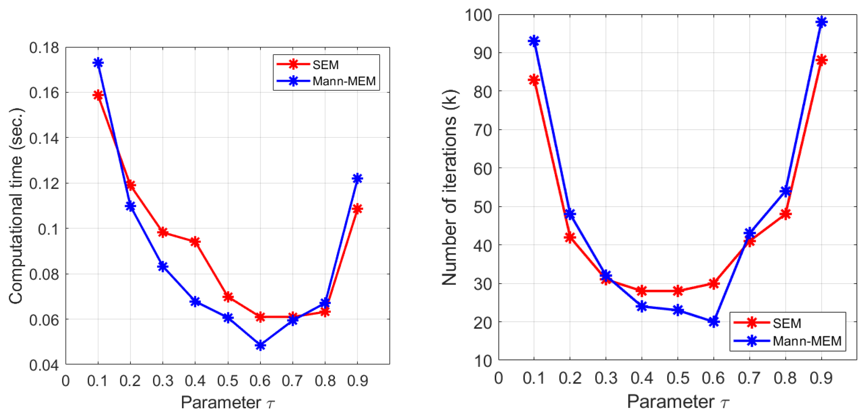
In Figure 1, we perform the experiments with varying the the stepsize $\tau >0$ in the two tested methods. With the same setting as above experiment and putting the inner-loop stepsize ${\lambda }_k=1.9/(k+1)$ for SEM and Mann-MEM. We observe that the best computational time for both SEM and Mann-MEM is obtained by the choice of $\tau =0.6$

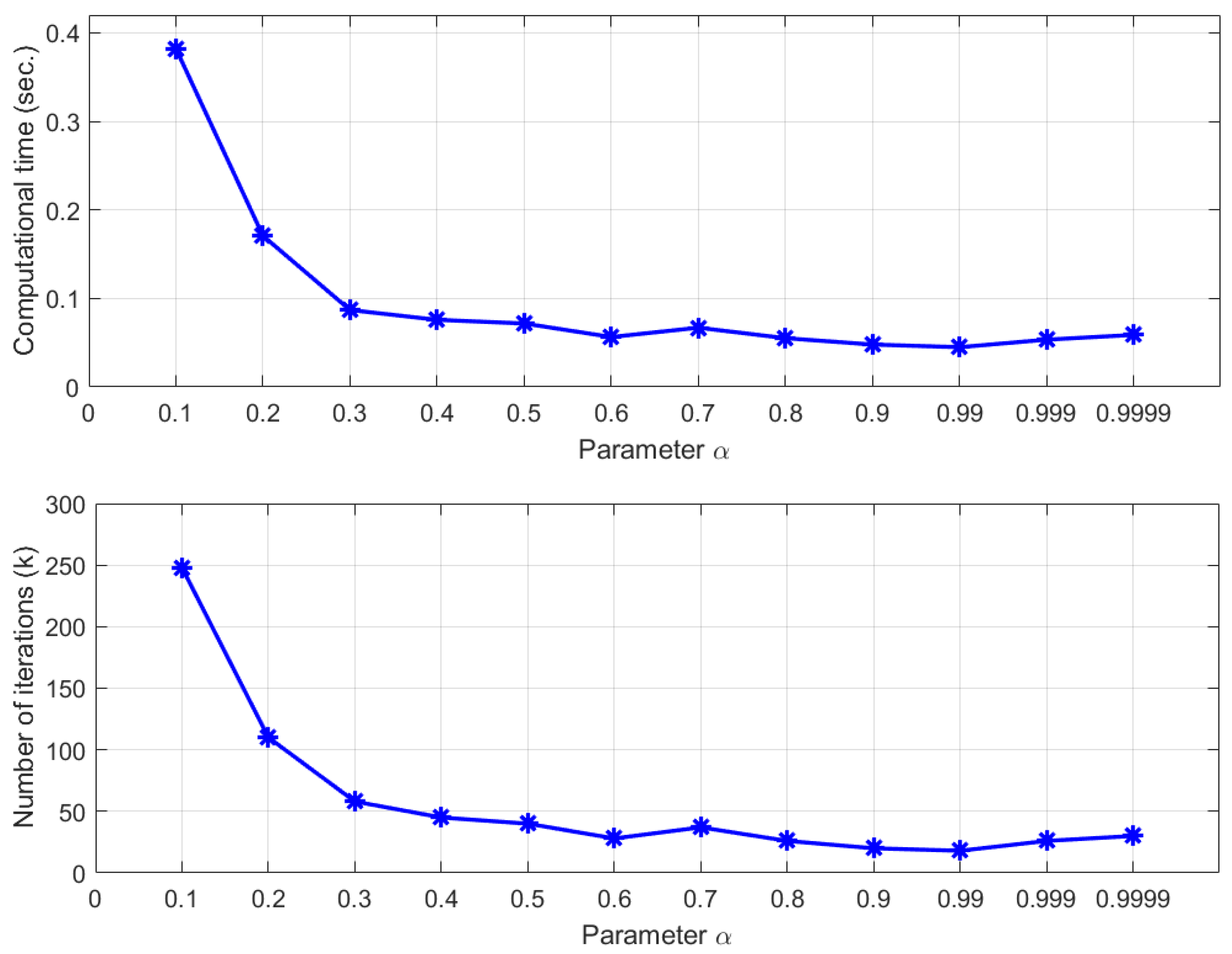
For more insight into the convergence behavior of Mann-MEM, we also consider the influence of the parameter $\alpha$ given in Mann-MEM. We put ${\lambda }_k=1.9/(k+1)$, and $\tau =0.6$, and the results are presented in Figure 2. It can be observed that the least computational time and the number of iterations are achieved when the parameter $\alpha$ is quite large, that is, the best algorithm’s performance is obtained by the choice of $\alpha =0.99$.

In the next experiment, we also considered the solving of the problem (19) by the aforementioned tested methods. We compare the methods for various dimensions n and the number of constraints m. We put vectors $a_i,i=1,\dots ,m$, whose coordinates are randomly chosen from the interval $[-m,m]$, positive real numbers $b_i=0.5,i=1,\dots ,m$, and the initial point $x_1$ is a vector whose coordinates are randomly chosen from the interval $[0,1]$. We set the point c to be a vector whose all coordinates are 1, and choose the best choices of parameters $\lambda =1.9$, and stepsize $\tau =0.6$ for SEM and $\lambda =1.9,\tau =0.6$, and $\alpha =0.99$ for Mann-MEM. In the following numerical experiments, in order to terminate SEM, we applied the following stopping criterion

$$\begin{array}{c}\hfill max\left\{\frac{\parallel x_{k+1}-x_k\parallel }{\parallel x_k\parallel +1},\parallel x_k-y_k\parallel \right\}\le {10}^{-5},\end{array}$$

(22)

and in order to terminate Mann-MEM, we applied the following stopping criterion

$$\begin{array}{c}\hfill max\left\{\frac{\parallel {\overline{x}}_{k+1}-{\overline{x}}_k\parallel }{\parallel {\overline{x}}_k\parallel +1},\parallel {\overline{x}}_k-y_k\parallel \right\}\le {10}^{-5}.\end{array}$$

(23)

We performed 10 independent tests for any collections of high dimensions $n=500,1000$, 2000, and 3000 and the number of constraints $m=50,100$, and 200. The results are presented in

Table 2. Behavior of SEM, Mann-MEM for different dimensions (n) and different number of constraints (m).

n	m	SEM		Mann-MEM
		Time	#(Iters)	Time	#(Iters)
500	50	38.7986	51.0	36.3368	51.2
	100	94.3647	51.0	88.4383	51.0
	200	248.4960	50.6	239.0405	51.0
1000	50	61.8089	52.0	58.6253	53.0
	100	143.5451	52.0	137.0350	53.0
	200	368.2668	52.0	344.8198	52.7
2000	50	123.3731	53.1	118.4089	54.0
	100	257.4444	53.0	245.7529	54.0
	200	604.0555	53.0	576.3775	54.0
3000	50	247.8855	54.0	242.2706	55.0
	100	452.0647	54.0	440.8821	55.0
	200	1070.5699	54.0	1031.5349	55.0

, where the average computational runtime and the average number of iterations for any collection of n and m are presented.

It is clear from Table 2 that Mann-MEM is more efficient than SEM in the sense that Mann-MEM requires less computation than SEM in the average computational runtime. One notable behavior is that for the case when m is quite large, Mann-MEM requires significantly below the average computational runtime. For each dimension, we observe that the larger problem sizes need more average computational runtime. This suggests that the use of the generalized segmenting averaging matrix is more efficient than SEM. In this situation, we can note that the essential superiority of Mann-MEM with respect to SEM is dependent on the optimal choice of the averaging matrix ${\left[{\alpha }_{k,j}\right]}_{k,j=1}^{\infty }$ which is, in our experiments, the generalized segmenting averaging matrix.

5. Some Concluding Remarks

The objective of this work was the solving of a variational inequality problem governed by a monotone and Lipschitz continuous operator. We associated to it the so-called Mann’s mean extragradient method, and proved weak convergence of the generated sequence of iterates to a solution to the considered problem. Numerical experiments show that under some suitable parameters, the proposed method has a better convergence behavior compared to the classical subgradient-extragradient method. For future work, some comments are in order.

(i)

Let us observe that the convergence of Mann-MEM requires us to know the Lipschitz constant L of the operator F, nevertheless, it is sometimes difficult to indicate exactly the Lipschitz constant, so that Mann-MEM and its convergence result can not be practically applicable. It is very interesting to consider a variant Mann-MEM with a variable stepsize ${\left\{{\tau }_k\right\}}_{k=1}^{\infty }$ in place of the fixed stepsize $\tau >0$ and the prior knowledge of L is not necessarily known.

(ii)

It can be noted that the superiority of Mann-MEM with respect to SEM is depended on the optimal choice of the averaging matrix ${\left[{\alpha }_{k,j}\right]}_{k,j=1}^{\infty }$. It is also very interesting to find more possible examples of averaging matrices satisfying the M-concentrating condition.