Abstract
The generalized bimodal distribution is especially efficient in modeling univariate data exhibiting symmetry and bimodality. However, its performance is poor when the data show important levels of skewness. This article introduces a new unimodal/bimodal distribution capable of modeling different skewness levels. The proposal arises from the recently introduced Lambert transformation when considering a generalized bimodal baseline distribution. The bimodal-normal and generalized bimodal distributions can be derived as special cases of the new distribution. The main structural properties are derived and the parameter estimation is carried out under the maximum likelihood method. The behavior of the estimators is assessed through simulation experiments. Finally, two applications are presented in order to illustrate the utility of the proposed distribution in data modeling in different real settings.
1. Introduction
Analysts often have to deal with data that exhibit bimodality; for example, when observing the size of worker ants in weaver ant colonies [1], the duration of volcanic eruptions [2], the amount of excretion of mercury in urine [3], the grain size in sintered Zirconia [4], or the amount of tropospheric water vapor in the tropics [5].
Two-component mixture distributions are usually used to model data that exhibit bimodality. These distributions have a very flexible density function (unimodal/bimodal), a highly valued feature when trying to model data in different real settings. However, one difficulty in working with them is that it is necessary to deal with the problem of the non-identifiability of their parameters, see McLachlan et al. [6] for more detail.
It is possible to find in the literature guidelines to deal with the problem of non-identifiability in a mixture distribution; for example, as suggested by Aitkin and Rubin [7], it is convenient to assume a certain restriction on the mixing parameter to evaluate the behavior of the maximum likelihood estimates. An alternative that has been considered in various studies is to impose restrictions on the components of the mixture distribution; for example, assuming that the components have the same variance. In this way, sub-families of mixture distributions with a simpler parametric structure (where the parameters are identifiable) are defined.
Taking into account certain restrictions for the components of a mixture distribution implies working with a sub-family that exhibits a less flexible density function than the unrestricted case. However, it is possible to find in the literature sub-families of two-component mixture distributions that have been shown to be useful in data modeling in various real settings. In this context, it is possible to find the generalized bimodal (GB) distribution originally proposed by Rao [8] and later studied as a special case of the bimodal symmetric distribution proposed in Sarma et al. [9].
A random variable X has a generalized bimodal distribution, denoted as , if its probability density function (pdf) is given by
and its cumulative distribution function (cdf) is given by
where is a shape parameter that controls bimodality and and denote the pdf and the cdf of the standard normal distribution, respectively.
It is easy to verify that Equation (1) corresponds to the pdf of a two-component mixture distribution with mixing parameter , for , one component having a standard normal distribution, and the other a standard bimodal-normal (BN) distribution. If , the Lambert generalized bimodal (LGB) distribution reduces to the BN distribution. Details on the structural properties of the BN distribution can be found in Hassan and Hijazi [10] and Elal-Olivero [11]. A class of generalized bimodal distributions that extends the GB distribution can be found in [12]. This class is defined by the cdf F(x) = Φ(x) − α(x) ϕ(x), where α(x) is a linear function of x. Thus, the GB distribution (with cdf given in Equation (2)) can be derived as a special case of the class proposed by [12] when α(x) = x/(1 + γ).
The parametric space bounded to the interval [0,2) for can be explained by the fact that the pdf given in Equation (1) is bimodal for any value of in such interval. However, we observe that the range of can be extended so that assumes values in the interval . In such case, it is possible to verify the following properties: The GB pdf is symmetric-bimodal when and symmetric-unimodal when . The GB distribution reduces to the bimodal-normal distribution when and tends to the standard normal distribution as .
The symmetry characteristic of the GB pdf can be considered a desirable characteristic in the analysis of certain data sets, but a limitation in the analysis of others. In the literature, it is possible to find different construction methods that allow generating an asymmetric distribution from a symmetric baseline distribution, see Azzalini [13], Eugene et al. [14], Cordeiro and de Castro [15], Ferreira and Steel [16], Goerg [17], and Alzaatreh et al. [18], among others.
Recently, Iriarte et al. [19] introduce the Lambert-F distribution generator defined as
where is an extra shape parameter and is the cdf of an arbitrary baseline distribution.
The transformation given in Equation (3) defines a new family of distributions more flexible in terms of skewness than the baseline distribution. Iriarte et al. [19] study two special cases of Equation (3), extending the classical exponential and Rayleigh distributions and showing that the hazard rate functions induced by this transformation can be understood as modifications in the early times of the baseline hazard rate functions.
In this article, we introduce a new unimodal/bimodal distribution that generalizes the GB distribution and is capable of modeling different levels of skewness. The proposal, called the Lambert generalized bimodal (LGB) distribution, arises from Equation (3) when considering a baseline GB distribution. The result is a new distribution that generalizes to the GB and BN distributions and that can serve as an alternative to other asymmetric bimodal distributions in the literature.
The article is organized as follows. In Section 2, we define the LGB random variable and derive the density and distribution functions. In Section 3, we describe the characteristics of unimodality, bimodality, asymmetry, and kurtosis. In addition, alias distributions are discussed. In Section 4, we consider the problem of parameter estimation using the maximum likelihood (ML) method. In Section 5, the behavior of the ML estimators and the utility of the proposed distribution are evaluated through simulation experiments. Section 6 presents two application examples illustrating the usefulness of the LGB distribution in real settings. Finally, the main conclusions are reported in Section 7.
2. The LGB Distribution
In this section, we introduce the LGB distribution and study some of its main properties.
2.1. LGB Random Variable
Definition 1.
A random variable X follows a Lambert generalized bimodal distribution, with location parameter , scale parameter and shape parameters , and , denoted as , if it can be represented as
where is the principal branch of the Lambert W function, is the standard generalized bimodal quantile function, and U is a uniform(0,1) random variable.
Remark 1.
The quantile function of the GB distribution does not have a closed analytical form. However, it can be calculated numerically from the cdf given in Equation (2).
Proposition 1.
Let . Then, the cdf of X is given by
Proof.
From the Equation (4), for , we have that
where is the inverse function of , that is, the standard GB cdf. Then, by definition of the Lambert W function, it follows that
and the result is obtained considering that , as . Finally, note that the analytical expression obtained for the cdf of X is valid for once . □
The pdf of X can be obtained in a straightforward way from the cdf given in Equation (5).
Corollary 1.
Let . Then, the pdf of X is given by
In accordance with Definition 1, note that Equations (5) and (6) reduce, respectively, to the cdf and pdf of the GB distribution when . Consequently, the LGB distribution can be understood as an extension with one extra parameter of the GB distribution. An interesting property of the LGB distribution is that its pdf corresponds to a modification in a multiplicative fashion of the GB pdf. If or , the GB pdf is modified in a multiplicative fashion by the expression , allowing asymmetric shapes for the LGB pdf.
Figure 1 shows some pdf curves for the LGB distribution considering different values of and . Here, it can be seen that the LGB pdf is bimodal symmetric when . Note that the parameter has an effect on the shape of the LGB pdf allowing unimodal or bimodal asymmetric shapes. This will be discussed in more detail in Section 3.
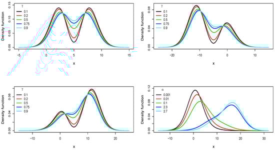
Figure 1.
Pdf curves for the LGB distribution for , , and in the top left panel; , , and in the top right panel; , , and in the bottom left panel; and , , and in the bottom right panel.
The quantile function (qf) of the LGB distribution can be easily derived by inverting Equation (5), considering steps very similar to those of the proof of Proposition 1. The resulting analytical expression for this function is given by
As the Lambert W function is included in different statistical software, Equation (7) can be easily computed. A code in the R programming language [20] is provided in Appendix A.
2.2. Related Distributions
In the previous section, it was shown that the LGB and GB distributions are nested distributions, with the GB distribution being a special case of the LGB distribution. Now, taking into account that the BN distribution is a special case of the GB distribution, we observe that the LGB distribution reduces to the BN distribution when and . Consequently, a new special case can be highlighted. If , the pdf given in Equation (6) reduces to
The pdf given in Equation (8) is bimodal symmetric or bimodal asymmetric depending on the value of . If , then Equation (8) reduces to the BN pdf. We refer to Equation (8) as the Lambert-bimodal normal (LBN) pdf. It is important to note that, unlike the LGB distribution, the pdf given in Equation (8) valued in the antimode is equal to 0 for all , , and .
We observe that the parameter induced by the Lambert-F transformation plays a determining role in the skewness of the LBN distribution. We also see that the LBN pdf can be understood as a modification in a multiplicative fashion of the BN pdf.
3. Shapes and Aliases
In this section, we discuss the forms of LGB distribution and analyze the possible existence of alias distributions for members of this LGB family.
3.1. Shapes
Let be the s-th derivative of the LGB pdf with respect to x, , we have
where
Thus, if , and if and are, respectively, critical points and inflection points of the pdf of X, then is a root of the equation
and a root of the equation
In the case , Equations (9) and (10) lead to establish that the LGB pdf is bimodal with modes given by , antimode given by , and abscissa of inflection points given by , with , where and .
In the case where , it is not possible to obtain closed expressions for the modes, antimode, and abscissa of inflection points. Therefore, these values must be obtained by solving Equations (9) and (10) by numerical procedures. Considering Equations (9) and (10) as functions of x, say and , respectively, we observe that
which means that Equation (9) has at least one root, associated with the unimodal case. Thus, the above also implies that the Equation (10) has at least two roots and, taking into account that
it follows that Equation (10) has at least one negative minimum value at , where satisfies the equation
Figure 2 shows a good summary of the shapes that the LGB pdf can take. In this figure, profiles are presented for the equations of critical points and inflection points, Equations (9) and (10), together with the corresponding LGB pdf. As in Figure 1 and Figure 2, it is observed that the LGB pdf can be unimodal or bimodal depending on the values of and , but here it is also observed that a unimodal LGB pdf can have two or four inflection points. In this sense, Equation (9) has one or three roots (depending on whether the pdf is unimodal or bimodal) and Equation (10) has two or four roots (four roots when the pdf is bimodal and two or four roots when the pdf is unimodal). In Figure 3, the regions of unimodality and bimodality established in the plane defined by the ranges of and are presented. This figure was drawn by solving Equation (9) using the uniroot.all function [21] in the R language [20].
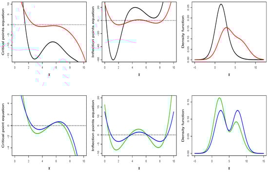
Figure 2.
Critical and inflection points and pdf curve for the distributions Lambert generalized bimodal (LGB) (5,2,1.5,0.005) (black curves), LGB (5,2,1.5,0.5) (red curves), LGB (5,2,0.5,0.5) (green curves), and LGB (5,2,0.5,1) (blue curves).
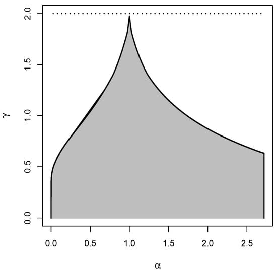
Figure 3.
Regions of unimodality (white region) and bimodality (gray region) for a LGB distribution.
3.2. Skewness and Kurtosis
Next, the skewness behavior of the LGB distribution is described. The behavior of the kurtosis is also described in the case in which the LGB distribution is unimodal. In this case, first the raw moments of the LGB distribution are derived and later the Fisher’s skewness and kurtosis coefficients are analyzed.
Proposition 2.
Let and . Then, for , the r-th raw moment of Z and X are given by and
where
Proof.
Corollary 2.
The mean and the variance of X are given by and , respectively.
Corollary 3.
The skewness () and kurtosis () coefficients of X are given by
Note that the r-th raw moment of the LGB distribution should be computed using numerical integration. Table 1 presents some values for the first four raw moments of the LGB distribution. Figure 4 (left panel) presents some curves for the skewness coefficient of the LGB distribution considering different values of γ; and α. In the right panel of the same figure, some curves for the kurtosis coefficient are presented when the LGB pdf is unimodal.

Table 1.
Some values for the first four raw moments of the LGB distribution considering different values of γ and α.
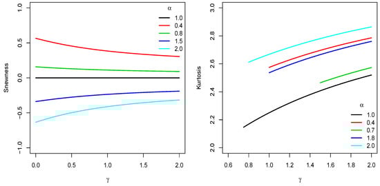
Figure 4.
Plots of the skewness and kurtosis coefficients of the LGB distribution.
In Table 1, we observe that the odd raw moments are 0 when α = 1, an expected result because in this case the LGB distribution is symmetric around μ. In the Figure 4, we observe that
- The LGB pdf is symmetric when α = 1, regardless of the value assumed by the parameter γ.
- The LGB distribution can be skewed (positively or negatively) depending on the value assumed by α. If or , then the LGB pdf is skewed and the skewness is also controlled by the parameter γ. However, the effect of γ on skewness is important when it assumes small values.
- If the LGB pdf is unimodal, then it is asymmetric.
- In the unimodal case, the excess kurtosis is less than 0; that is, the LGB distribution is a platykurtic distribution.
In the case where , we observe from Equations (7) and (11) that the skewness of the LGB distribution is positive if γ and α satisfy the inequality
On the other hand, values of γ and α () that do not satisfy the previous inequality are related to a negative skewness.
Based on these last results, together with the results of Section 3.1, we observe that the LGB distribution can be considered as a feasible alternative for modeling data exhibiting asymmetry and uni/bimodality. In this way, the LGB distribution can be used in the analysis of random phenomena raised in various areas of knowledge. Below, we describe some situations in which the LGB distribution could be used: (1) In entomology, volcanology, medicine, materials science, and climatology, according to the scenarios exposed at the beginning of Section 1. (2) In meteorology; for example, when analyzing wind speed data in certain geographic regions that tend to have two speed spikes per day. (3) In astronomy; for example, when analyzing data associated with certain solar wind parameters. Studies based on annual measurements have shown that the distribution of solar wind speed (as well as those of other parameters such as proton density, temperature and magnetic field) can exhibit bimodality. (4) In population dynamics. It is well known that the interactions between the characteristics of the individuals that make up a certain population can produce changes in the distribution of the size of the individuals, including changes that lead to a bimodal distribution.
3.3. Alias Distributions
Previously, it was noted that the original range for the parameter γ of the GB distribution can be extended so that γ assumes values in the interval [0,∞). In this way, the normal distribution can be obtained as a limiting case of the GB distribution. Despite this interesting property, we have considered the range bounded to the interval [0,2) for the parameter γ of the LGB distribution. The rationale for this is to avoid alias distributions for some members of the LGB distribution, that is, avoid distributions that are virtually identical in relation to minimizing the Kullback–Leibler divergence [22]. The Kullback–Leibler divergence measures the degree of divergence between the distributions of two random variables. For two LGB, random variables consider the following proposition.
Proposition 3.
Let and , where , . Then, the Kullback–Leibler divergence is given by
where and is as in Equation (6).
Proof.
From the definition of the Kullback–Leibler divergence, we obtain
where the expectation is taken with respect to . Thus, the result is obtained by considering the change of variable , once can be written as . □
Considering known, minimizing Equation (13) with respect to is equivalent to solving a nonlinear system of four equations, see Appendix B.
We observe that the existence of alias distributions in the LGB distributions family is related to its skewness behavior when considering that γ can also assume values greater than or equal to 2. In the case , it can be verified that the LGB family is unimodal regardless of the value of α. In Figure 4 (left panel), it is observed that the skewness of the LGB distribution is positive for those values of . However, we observe that the skewness can become negative if α assumes a value close to 0, once γ has assumed a value greater than 2 that is large enough. This favors the existence of alias distributions for certain unimodal members of the family, as it suggests that a negative skewness value may be associated with two different values of α. Under this scenario, it must be taken into account that this is very serious when both members of the family are unimodal, as it would be enough to make an adequate consideration of the locations and scales so that the members are virtually identical.
To exemplify the above, consider the LGB family member specified by , , , and , which has a unimodal shape and slightly negative skewness. Now, consider also a LGB distributions subfamily where μ and σ are unknown: and , respectively. In this scenario, the members of the subfamily have unimodal shape and the same skewness value as the fully specified distribution. In Figure 5, we graphically represent the behavior of the skewness for the fully specified distribution (in blue color) and for the LGB subfamily (in red color). In this figure (left panel), it is observed that the skewness is negative only for when , while the skewness can be negative for both values of α (0.001 and 1.6) if γ is sufficiently large (center panel). Notice that both skewness curves tend to as . Therefore, among the members of the LGB distributions subfamily, it is possible to find an alias distribution for the fully specified distribution by considering certain values for the location and scale parameters. These values are and , which are obtained by minimizing the Kullback–Leibler divergence given in Equation (13), where the minimum value of is 0.0008. The right panel of Figure 5 shows the pdf curves for the LGB() distribution (black color) and for some members of the LGB family with , , , and different values of γ. Notice that the pdfs represented by the dashed lines approach the black curve as γ grow toward the value 1000, so that the distributions LGB ( and LGB () are virtually identical. Figure 6 shows the Kullback–Leibler divergence curve as functions of and for and , where it can be seen that the Kullback–Leibler divergence is minimized precisely at and .
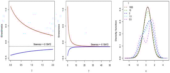
Figure 5.
Top and center panels: Skewness curves for two LGB distributions with in blue color and in red color. Right panel: Pdf curves for an LGB (0,1,1000,1.6) distribution (in black color) and four LGB distributions specified by , , , and different values of .
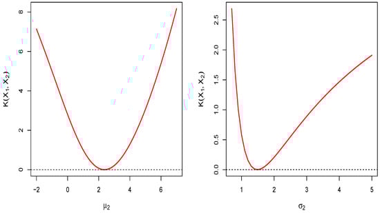
Figure 6.
Kullback–Leibler divergence curve for and as a function of in the left panel and as a function of in the right panel.
Returning to Figure 5 (right panel), it is clearly observed that those pdfs related to a value of less than 2 are not alias distributions of the LGB (0,1,1000,1.6) distribution. Finally, based on the minimization of Equation (13), we analyze the existence of alias distributions in scenarios where is less than 2 and in others where it is greater than 2. In each scenario, and , , , where is known and minimizes Equation (13). Specifically, the scenarios considered are the following: Scenario A: , , where . Scenario B: , , where . Scenario C: , , where . Scenario D: , , where . Scenario E: , , where . Scenario F: , , where .
Table 2 shows the values of the mean, variance, skewness, number of critical points, and inflection points for the distributions of the random variables and in each scenario. Here, we observe that in scenarios E and F (when ) the values for the two distributions are very similar, so that the distributions of and are virtually identical. In contrast, in scenarios A to D (when ) the values differ especially in the number of critical points and inflection points, and therefore the distribution of is not an alias of the distribution of . Graphical comparisons of the pdf’s of and can be seen in Appendix C.
Table 2.
Mean, variance, skewness, and amounts of critical points and inflection points of the pdf for the distributions of and in scenarios A to F.
4. Maximum Likelihood Estimator
In this section, we deal with the problem of parameter estimation in the LGB distribution under the maximum likelihood (ML) method.
If , then (for ’) the log-likelihood is given by
where
Thus, the elements of the score vector are
For a random sample from , we observe that the ML estimator ’ for ’ cannot be expressed in closed form. The solution of the likelihood equations gives rise to a system of four nonlinear equations (See Appendix D) that must be solved with the help of some computational routine in search of ML estimates.
In this case, as the ML estimators do not have a closed form, a good alternative to obtain ML estimates is to solve the following optimization problem,
where is given in Equation (14). We solved (15) using the function optim of the R language [20] and, specifically, the L-BFGS-B algorithm [23] was applied. This algorithm requires the declaration of a feasible starting point in the parametric space to start the iterative process. Considering that the bimodal-normal distribution is a special case of the LGB distribution, we verify through simulation experiments that (), where is the mean of the observations and the corresponding standard deviation, is a good starting point.
Under regularity conditions, the asymptotic distribution of is , where is the expected information matrix. As the function is not simple, it is not easy to obtain the analytical expression of this matrix. However, we obtain an approximation from the observed information matrix, whose elements are computed as minus the second partial derivatives of the log-likelihood function with respect to all the parameters (evaluated at the ML estimates). Thus, for a random sample from , the observed information matrix is given by
with , , and , where the analytical expressions of the second partial derivatives are presented in Appendix E.
5. Simulation Studies
In the analysis of data exhibiting bimodality, it is common to use a two-component mixture normal (MN) distribution. In this section, we initially carry out a simulation study to evaluate the behavior of the ML estimators of the LGB distribution parameters. Subsequently, we conducted a second simulation study in order to evaluate the usefulness of the LGB distribution in a context where the MN distribution performs well.
5.1. First Simulation Study
In this study, 1000 random samples from the LGB distribution were generated considering the sample sizes n = 100, 200, 300, 500, and 1000 in the following two scenarios:
- Scenario A: , , and .
- Scenario B: , , and .
Simulated random samples were generated using the qf given in Equation (7). The LambertW package [24] in the R language was used to compute the principal branch of the Lambert W function. A code in the R language is provided in Appendix A.
For each simulated sample, we obtain the ML estimates by solving (15) under the considerations mentioned in Section 4. Table 3 reports the average estimate (AE), the empirical standard deviation (SD), and the root of the mean square error (RMSE) for the 1000 estimates obtained in each scenario and sample size considered. Table 4 reports the average of the asymptotic standard error (SE) for the ML estimates along with the coverage probability (CP) of the 95% asymptotic confidence intervals.
Table 3.
Averages (AE), standard deviations (SD), and root of the simulated mean square errors (RMSE) for the estimates of , , , and of the LGB distribution.
Table 4.
Averages of asymptotic standard errors (SE) and coverage probabilities (CP) for the estimates of , , , and for the LGB distribution.
Table 3 indicates that the AEs tend to be close to the true values of the parameters as the sample size increases. The SDs and RMSEs are close and decrease towards 0 as the sample size increases, as expected in the standard asymptotic theory. Table 4 indicates that the SEs are close to the SDs and RMSEs given in Table 3. As expected, the SEs decrease towards 0 and the CPs converge to the nominal values used to construct the confidence intervals as the sample size increases.
5.2. Second Simulation Study
In the first place, 1000 random samples from MN distribution were generated considering the sample sizes n = 50, 100, 200, 300 and the following four scenarios: Scenario A, , , , , and . Scenario B, , , , , and . Scenario C, , , , and . Scenario D, , , , , and .
For each simulated sample, the LGB and MN distributions are fitted via the ML method using the optim function in R language. Subsequently, based on the Akaike Information Criterion (AIC) [25], Corrected Akaike Information Criterion (CAIC) [26], and Bayesian Information Criterion (BIC) [27], the proportions where the AIC, CAIC, and BIC values are lower in the LGB distribution are calculated. We call this the hit rate for the LGB distribution. In addition, the modified Cramer–von Mises () and Anderson–Darling () statistics [28] are calculated for the LGB distribution in order to test the hypothesis is a random sample from a LGB population, where the parameters have been estimated by the ML method. Thus, we calculate the rate of simulated samples where is not rejected, which we call the non-rejection rate.
Finally, considering a procedure analogous to the one described above, we simulate random samples from the LGB distribution and calculate the hit and non-rejection rates for the MN distribution. The scenarios considered here are the following: Scenario A, , , , and . Scenario B, , , , and . Scenario C, , , , and . Scenario D, , , , and .
Table 5 and Table 6 report the hit and non-rejection rates for the LGB and MN distributions, respectively. In Table 5, we observe that the non-rejection rates are high, which means that a considerable proportion of samples generated from the MN distribution can be appropriately fitted with the LGB distribution. On the other hand, we observe that the hit rates are high, exceeding the value 0.5, even in moderate sample sizes, . Note that the non-rejection rates decrease considerably in scenario D as the sample size increases and that the hit rates are lower than the other scenarios. This is because the samples are generated from a MN population where the scales and are considerably different. This shows that the LGB distribution can perform well in settings where the MN distribution is used and where the estimates for and in this distribution are similar.
Table 5.
Non-rejection rate based on modified statistics and and hit rates based on the AIC, CAIC, and BIC for the LGB distribution, when the data are simulated from the MN distribution.
Table 6.
Non-rejection rate based on modified statistics and and hit rates based on the AIC, CAIC, and BIC for the MN distribution, when the data are simulated from the LGB distribution.
In Table 6, we observe that the non-rejection rates are very high, which was expected as the MN distribution has one more parameter than the LGB distribution. This means that a very considerable proportion of samples generated from a LGB population can be appropriately fitted with the MN distribution. However, due to having one more parameter, the hit rates in the different scenarios are small, as the AIC, CAIC, and BIC values depend on the number of parameters of the distribution. Therefore, it can be expected that in a possible real setting where both distributions appropriately fit a certain dataset, the information criteria AIC, CAIC, and BIC will provide favorable indications for the use of the LGB distribution due to the fact of having to estimate a smaller amount of parameters.
6. Data Analysis
In this section, two applications are presented in order to illustrate the usefulness of the LGB distribution and its special cases in data modeling in different real settings. Other symmetric/asymmetric unimodal/bimodal distributions are also considered to illustrate that the LGB distribution or some of its special cases may have a better fit than other distributions in the literature. Specifically, the odd log-logistic skew-normal (OLLSN) [29] and gamma sinh-Cauchy (GSC) [30] distributions are considered. Like the LGB distribution, these distributions have four parameters: two shape parameters (which together control skewness and bimodality), a location parameter, and a scale parameter. A mixture distribution of two normal components (MN) [6] is also included into the analysis as it is a commonly used distribution for analyzing data exhibiting bimodality.
- The first dataset corresponds to 188 observations on the inflation rate (in %) registered quarterly between the years 1950 and 1996 in Canada. This dataset can be found with the name Tbrate in the R language [31].
- The second dataset refers to 128 observations on the electrical resistance (in ohms) of nectarine fruits. This data can be found with the name fruitohms in the R language [32].
For the datasets described above, we test hypothesis : the data have exactly one mode versus the alternative hypothesis : the data have at least two modes. For this, we consider the excess mass test [33] using the modetest function in R language [34]. For the inflation rate data, the observed statistic was 0.05 with a p-value equal to 0.05. For the electrical resistance data, these values were 0.074 and 0.01, respectively. Thus, at a significance level equal to 0.05, in both datasets is rejected; that is, the distributions of the inflation rate and electrical resistance data are at least bimodal.
We compared the distributions fitted by the ML method using the information criteria AIC, CAIC, and BIC. We also calculate the statistics and to test the hypothesis is a random sample from a continuous distribution , where is known but is unknown. In these tests, is rejected at a significance level equal to 0.05 if and .
Table 7 reports the ML estimates with the corresponding standard errors for each distribution fitted to the inflation rate and electrical resistance data. In addition, the values associated with the statistics and and with the information criteria are reported.
Table 7.
The ML estimates and their standard errors (in parentheses) for each distribution fitted to the inflation rate and electrical resistance data and the values of the statistics and and of the information criteria.
In Table 7, with respect to the inflation rate data, based on the values of the statistics and , it can be seen that the hypothesis that the data correspond to an observed random sample of the GSC, GB, LBN, or BN distributions is rejected at a significance level equal to 0.05. In addition, it can be seen that the LGB distribution is the one with the lowest AIC, CAIC, and BIC values among the fitted distributions, indicating that this distribution should be selected over the others for the modeling of these data.
With respect to the electrical resistance data, it is observed that the hypothesis that the data correspond to an observed random sample of the OLLSN, GB, BN, or GSC distributions is rejected at a significance level equal to 0.05. Note that the AIC, CAIC, and BIC values for the LGB, MN, and LBN distributions are close, the values associated with the LBN distribution being slightly lower. Thus, the LBN distribution (which has a smaller parametric dimension than the LGB and MN distributions) is capable of fitting the electrical resistance data as well as the LGB and MN distributions.
In the left panels of Figure 7 and Figure 8, the histograms of inflation rate and electrical resistance are displayed along with the fitted densities. In the right panels of the same figures, the empirical cdf and the fitted cdf’s are compared. In these plots, we see that the LGB distribution fits the inflation rate data appropriately, while the LBN distribution fits the electrical resistance data appropriately. Note that the LGB and LBN distributions have one and two fewer parameters, respectively, than the MN distribution, and that despite this fact they are capable of presenting good fits to the analyzed data.
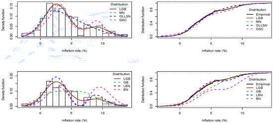
Figure 7.
Left panels: Histogram for inflation rate data and the fitted pdf curves via the ML method. Right panels: Empirical cdf for the inflation rate data and the fitted cdf curves.
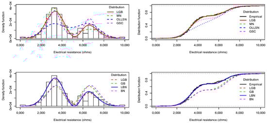
Figure 8.
Left panels: Histogram for electrical resistance data and the fitted pdf curves via the ML method. Right panels: Empirical cdf for the electrical resistance data and the fitted cdf curves.
7. Final Comments
This article introduces a new symmetric/asymmetric unimodal/bimodal distribution called the Lambert generalized bimodal (LGB) distribution. Some special cases of the LGB distribution are discussed. One of the special cases, the Lambert-bimodal normal (LBN) distribution, can be considered as an alternative to other symmetric/asymmetric bimodal distributions, including the LGB distribution. The LGB distribution arises using the Lambert-F transformation when the generalized bimodal distribution is considered as baseline distribution. We study the main structural properties of the LGB distribution, such as the pdf, cdf, qf, and raw moments that are used for a description of the skewness and kurtosis characteristics. Parameter estimation of the LGB distribution is discussed using the ML method. Through simulation experiments, we observe that the ML method provide acceptable estimates of the parameters of the LGB distribution. Furthermore, through simulation experiments, we observed that the LGB distribution can adequately fit datasets generated from the mixture normal distribution, despite having one less parameter. Finally, two applications that illustrate that the LGB distribution and the LBN especial case can present a better fit of data in real settings than other symmetric/asymmetric unimodal/bimodal distributions such as the odd log-logistic skew-normal distribution (OLLSN), gamma sinh-Cauchy (GSC), and mixture normal (MN) distributions.
As a final consideration, we leave the question open, does the LGB distribution have an intuitive stochastic representation? In the literature, it is possible to find distribution families that have an attractive intuitive generation mechanism, such as the skew-elliptical (SE) distributions [35] and the closed-skew-normal (CSN) distribution [36]. According to Loperfido et al. [37], any linear combination of the largest and smaller component of a bivariate, exchange elliptical random vector has a skew-elliptical distribution. According to Loperfido [38], any order statistic from a random vector with exchangeable normal distribution has a closed-skew-normal distribution. As far as we know, no similar property is known for the Lambert-F distributions class or for some of its special cases.
Author Contributions
Conceptualization, Y.A.I. and M.d.C.; Formal analysis, Y.A.I., M.d.C., and H.W.G.; Investigation, Y.A.I., M.d.C., and H.W.G.; Methodology, Y.A.I. and H.W.G.; Software, Y.A.I.; Supervision, M.d.C. and H.W.G.; Validation, H.W.G.; All of the authors contributed significantly to this research article. All authors have read and agreed to the published version of the manuscript.
Funding
The research of Y. A. Iriarte was funded by CONICYT PAI/INDUSTRIA 79090016, Chile. This work was partially done during M. de Castro’s visit to the Universidad de Antofagasta, supported by MINEDUC-UA Project, code ANT1856, Chile. The work of M. de Castro is partially funded by CNPq, Brazil. The research of H.W. Gómez was supported by Grant SEMILLERO UA-2021 (Chile).
Acknowledgments
The authors would like to thank the editor and the anonymous referees for their comments and suggestions, which significantly improved our manuscript.
Conflicts of Interest
The authors declare no conflicts of interest.
Abbreviations
The following abbreviations are used in this manuscript:
| Probability density function | |
| cdf | Cumulative distribution function |
| qf | Quantile function |
| AIC | Akaike information criterion |
| CAIC | Corrected Akaike information criterion |
| BIC | Bayesian informetion criterion |
| MN | Mixture normal |
| GB | Generalized bimodal |
| GSC | Gamma sinh-Cauchy |
| OLLSN | Odd log-logistic skew-normal |
| LGB | Lambert generalized bimodal |
Appendix A. R Codes to Compute the qf of the LGB Distribution and Generate Pseudo-Random Numbers
+ qgbimodal <- function(p,gamma){
+ n = length(p)
+ f = rep(0,n)
+ for(i in 1:n){
+ f[i] = uniroot(function(x,gamma)pnorm(x)-x/(gamma+1)*dnorm(x)-p[i],
+ c(-1e+4,1e+4),gamma=gamma)$‘root‘
+ }
+ return(f)
+ }
+
+ library(LambertW)
+
+ qLGB <- function(p,mu,sigma,gamma,alpha){
+ if(alpha==1){
+ mu+sigma*qgbimodal(p,gamma)
+ }else{
+ pp = 1/log(alpha)*W(log(alpha)*(p-1)/alpha)+1
+ mu+sigma*qgbimodal(pp,gamma)
+ }
+ }
+
+ n <- 100; p <- runif(n); mu <- 5; sigma <- 3; gamma <- 0.5; alpha <- 1.5
+ x <- qLGB(p,mu,sigma,gamma,alpha)
Appendix B. System of Equations to Minimize the Kullback–Leibler Divergence with Respect to θ2
Let and , , , where is known and is unknown. Then, the Kullback–Leibler divergence, , has a minimum value at , with , where satisfies the system of equations
where
Appendix C. Graphical Comparison of the pdf of X1 and X2 in Scenarios A to F

Figure A1.
Pdf curves of (black solid line) and (red dashed line) in scenarios A to F.
Figure A1.
Pdf curves of (black solid line) and (red dashed line) in scenarios A to F.

Appendix D. System of Equations to Obtain the ML Estimates Based on a Random Sample of Size n from a LGB(μ, σ, γ, α) Population
Let be a random sample of , where is unknown. Then, the ML estimate of is a root of the system of equations
Appendix E. Second Partial Derivatives of the Log-Likelihood Function for a Single Observation of the LGB Distribution
If and , the second partial derivatives of the log-likelihood function with respect to all the parameters are given by
References
- Weber, N.A. Dimorphism in the African Oecophylla worker Nd an anomaly (Hym.: Formicidae). Ann. Entomol. Soc. Am. 1946, 39, 7–10. [Google Scholar] [CrossRef]
- Azzalini, A.; Bowman, A.W. A look at some data on the Old Faithful Geyser. Appl. Statist. 1990, 39, 357–365. [Google Scholar] [CrossRef]
- Ely, J.T.A.; Fudenberg, H.H.; Muirhead, R.J.; LaMarche, M.G.; Krone, C.A.; Buscher, D.; Stern, E.A. Urine mercury in micromercurialism: Bimodal distribution and diagnostic implications. Bull. Environ. Contam. Toxicol. 1999, 63, 553–559. [Google Scholar] [CrossRef]
- Dierickx, D.; Basu, B.; Vleugels, J.; Van der Biest, O. Statistical extreme value modeling of particle size distributions: Experimental grain size distribution type estimation and parameterization of sintered zirconia. Mater. Character 2000, 45, 61–70. [Google Scholar] [CrossRef]
- Zhang, C.; Mapes, B.E.; Soden, B.J. Bimodality in tropical water vapor. Q. J. R. Meteorol. Soc. 2004, 129, 2847–2866. [Google Scholar] [CrossRef]
- McLachlan, G.J.; Lee, S.X.; Rathnayake, S.I. Finite mixture models. Annu. Rev. Stat. Appl. 2019, 6, 355–378. [Google Scholar] [CrossRef]
- Aitkin, M.; Rubin, D.B. Estimation and hypothesis testing in finite mixture models. J. Roy. Statist. Soc. Ser. B 1985, 47, 67–75. [Google Scholar] [CrossRef]
- Rao, K.S. On a bivariate bimodal distribution. In Proceedings of the ISPS Annual Conference, Delhi, India, 1987. [Google Scholar]
- Sarma, P.V.S.; Rao, S.K.S.; Rao, R.P. On a family of bimodal distributions. Sankhya Ser. B 1990, 52, 287–292. [Google Scholar]
- Hassan, M.Y.; Hijazi, R.H. A bimodal exponential power distribution. Pak. J. Statist. 2010, 2, 379–396. [Google Scholar]
- Elal-Olivero, D. Alpha-skew-normal distribution. Proyecciones 2010, 29, 224–240. [Google Scholar] [CrossRef]
- Hassan, M.Y.; El-Bassiouni, M.Y. Bimodal Skew-Symmetric Normal Distribution. Commun. Stat.—Theory Methods 2016, 45, 1527–1541. [Google Scholar] [CrossRef]
- Azzalini, A. A class of distributions which includes the normal ones. Scand. J. Stat. 1985, 12, 171–178. [Google Scholar]
- Eugene, N.; Lee, C.; Famoye, F. Beta-normal distribution and its applications. Commun. Stat. Theory Methods 2002, 31, 497–512. [Google Scholar] [CrossRef]
- Cordeiro, G.M.; de Castro, M. A new family of generalized distributions. J. Stat. Comput. Simul. 2011, 81, 883–898. [Google Scholar] [CrossRef]
- Ferreira, J.T.S.; Steel, M.F.J. A constructive representation of univariate skewed distributions. J. Am. Stat. Assoc. 2006, 101, 823–829. [Google Scholar] [CrossRef]
- Goerg, G.M. Lambert W random variables-a new family of generalized skewed distributions with applications to risk estimation. Ann. Appl. Stat. 2011, 5, 2197–2230. [Google Scholar] [CrossRef]
- Alzaatreh, A.; Lee, C.; Famoye, F. A new method for generating families of continuous distributions. Metron 2013, 71, 63–79. [Google Scholar] [CrossRef]
- Iriarte, Y.A.; de Castro, M.; Gómez, H.W. Lambert-F distributions class: An alternative family for positive data analysis. Mathematics 2020, 8, 1398. [Google Scholar] [CrossRef]
- R Core Team. R: A Language and Environment for Statistical Computing; R Foundation for Statistical Computing: Vienna, Austria, 2019. [Google Scholar]
- Soetaert, K. rootSolve: Nonlinear Root Finding, Equilibrium and Steady-State Analysis of Ordinary Differential Equations. R-Package Version 1.6. 2009. Available online: https://CRAN.R-project.org/package=rootSolve (accessed on 3 February 2021).
- Hutson, A.D.; Vexler, A. A cautionary note on beta families of distributions and the aliases within. Am. Stat. 2017, 72, 121–129. [Google Scholar] [CrossRef]
- Byrd, R.H.; Lu, P.; Nocedal, J.; Zhu, C. A limited memory algorithm for bound constrained optimization. SIAM J. Sci. Comput. 1995, 16, 1190–1208. [Google Scholar] [CrossRef]
- Goerg, G.M. LambertW: Probabilistic Models to Analyze and Gaussianize Heavy-Tailed, Skewed Data. R Package Version 0.6.4. 2016. Available online: https://CRAN.R-project.org/package=LambertW (accessed on 3 February 2021).
- Akaike, H. A new look at the statistical model identification. IEEE Trans. Automat. Contr. 1974, 19, 716–723. [Google Scholar] [CrossRef]
- Bozdogan, H. Model selection and Akaike’s information criterion (AIC): The general theory and its analytical extension. Psychometrika 1987, 52, 345–370. [Google Scholar] [CrossRef]
- Schwarz, G. Estimating the dimension of a model. Ann. Stat. 1978, 6, 461–464. [Google Scholar] [CrossRef]
- Chen, G.; Balakrishnan, N. A general purpose approximate goodness-of-fit test. J. Qual. Technol. 1995, 27, 154–161. [Google Scholar] [CrossRef]
- da Silva Braga, A.; Cordeiro, G.M.; Ortega, E.M.M. A new skew-bimodal distribution with applications. Commun. Stat. Theory Methods. 2018, 47, 2950–2968. [Google Scholar] [CrossRef]
- Gómez, Y.M.; Gómez-Déniz, E.; Venegas, O.; Gallardo, D.I.; Gómez, H.W. A new skew-bimodal distribution with applications. Symmetry 2019, 11, 899. [Google Scholar] [CrossRef]
- Croissant, Y.; Graves, S. Ecdat: Data Sets for Econometrics. R Package Version 0.3-4. 2019. Available online: https://CRAN.R-project.org/package=Ecdat (accessed on 3 February 2021).
- Maindonald, J.H.; John Braun, J.W. DAAG: Data Analysis and Graphics Data and Functions. R Package Version 1.22.1. 2019. Available online: https://CRAN.R-project.org/package=DAAG (accessed on 3 February 2021).
- Ameijeiras-Alonso, J.; Crujeiras, R.M.; Rodríguez-Casal, A. Mode testing, critical bandwidth and excess mass. Test 2019, 28, 900–919. [Google Scholar] [CrossRef]
- Ameijeiras-Alonso, J.; Crujeiras, R.M.; Rodríguez-Casal, A. Multimode: An R Package for Mode Assessment. arXiv 2018, arXiv:1803.00472. [Google Scholar]
- Branco, M.D.; Dey, D.K. A general class of multivariate skew-elliptical distributions. J. Multivar. Anal. 2001, 79, 99–113. [Google Scholar] [CrossRef]
- González-Farías, G.; Domínguez-Molina, A.; Gupta, A.K. Additive properties of skew-normal random vectors. J. Stat. Plan. Inference 2004, 126, 521–534. [Google Scholar] [CrossRef]
- Loperfido, N.; Navarro, J.; Ruiz, J.M.; Sandoval, C.J. Some relationships between skew-normal distributions and order statistics from exchangeable normal random vectors. Commun. Stat. Theory Methods 2007, 36, 1719–1733. [Google Scholar] [CrossRef]
- Loperfido, N. A note on skew-elliptical distributions and linear functions of order statistics. Stat. Probab. Lett. 2008, 78, 3184–3186. [Google Scholar] [CrossRef]


Publisher’s Note: MDPI stays neutral with regard to jurisdictional claims in published maps and institutional affiliations. |
© 2021 by the authors. Licensee MDPI, Basel, Switzerland. This article is an open access article distributed under the terms and conditions of the Creative Commons Attribution (CC BY) license (http://creativecommons.org/licenses/by/4.0/).