
A New Oversampling Method Based on the Classification Contribution Degree


Abstract
1. Introduction
2. Methodology
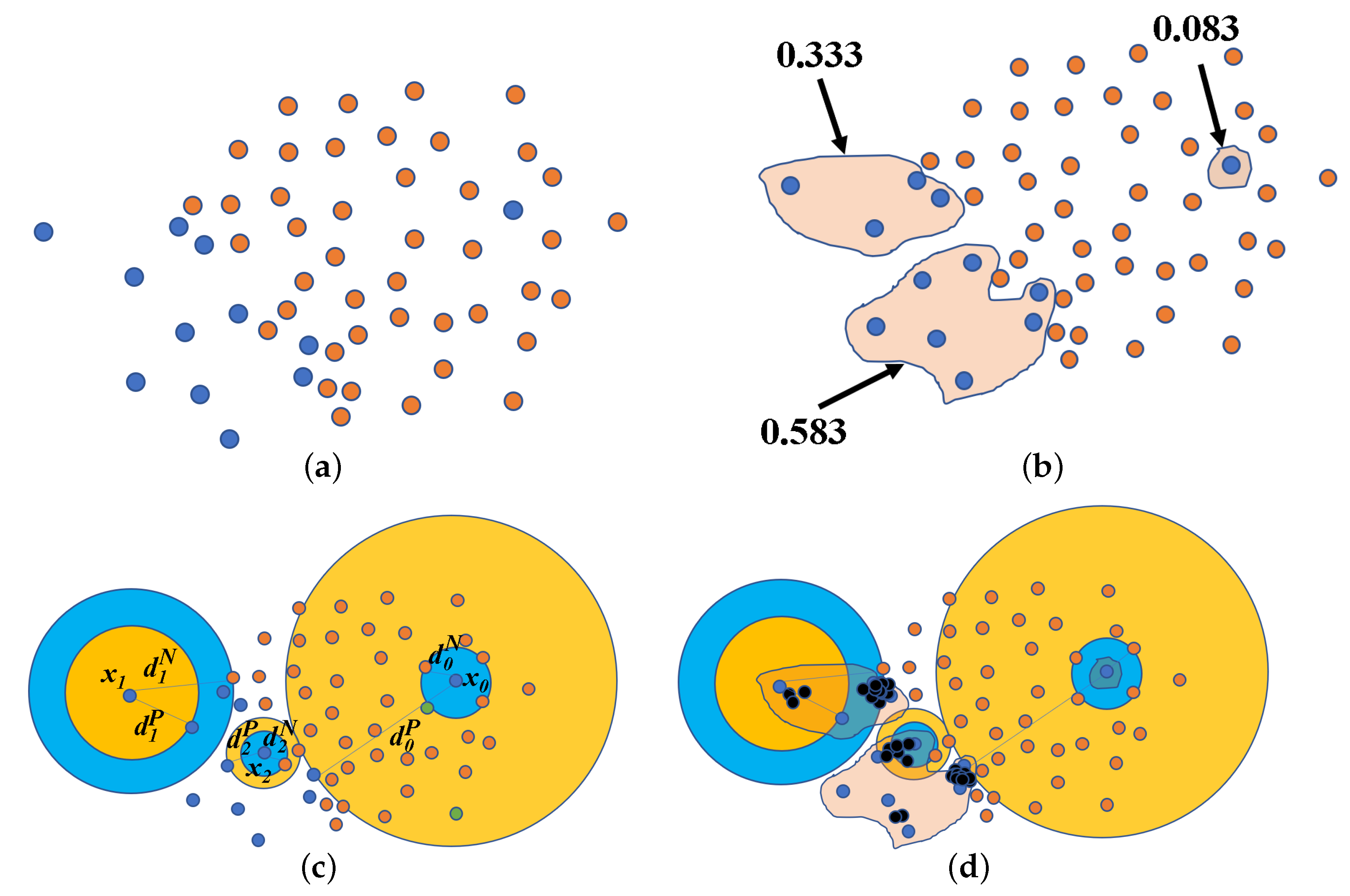
2.1. Safe Neighborhood and Classification Contribution Degree
2.2. Oversampling Based on the Classification Contribution Degree
3. Results and Discussion
3.1. Datasets Description and Experimental Evaluation
3.2. Experimental Method
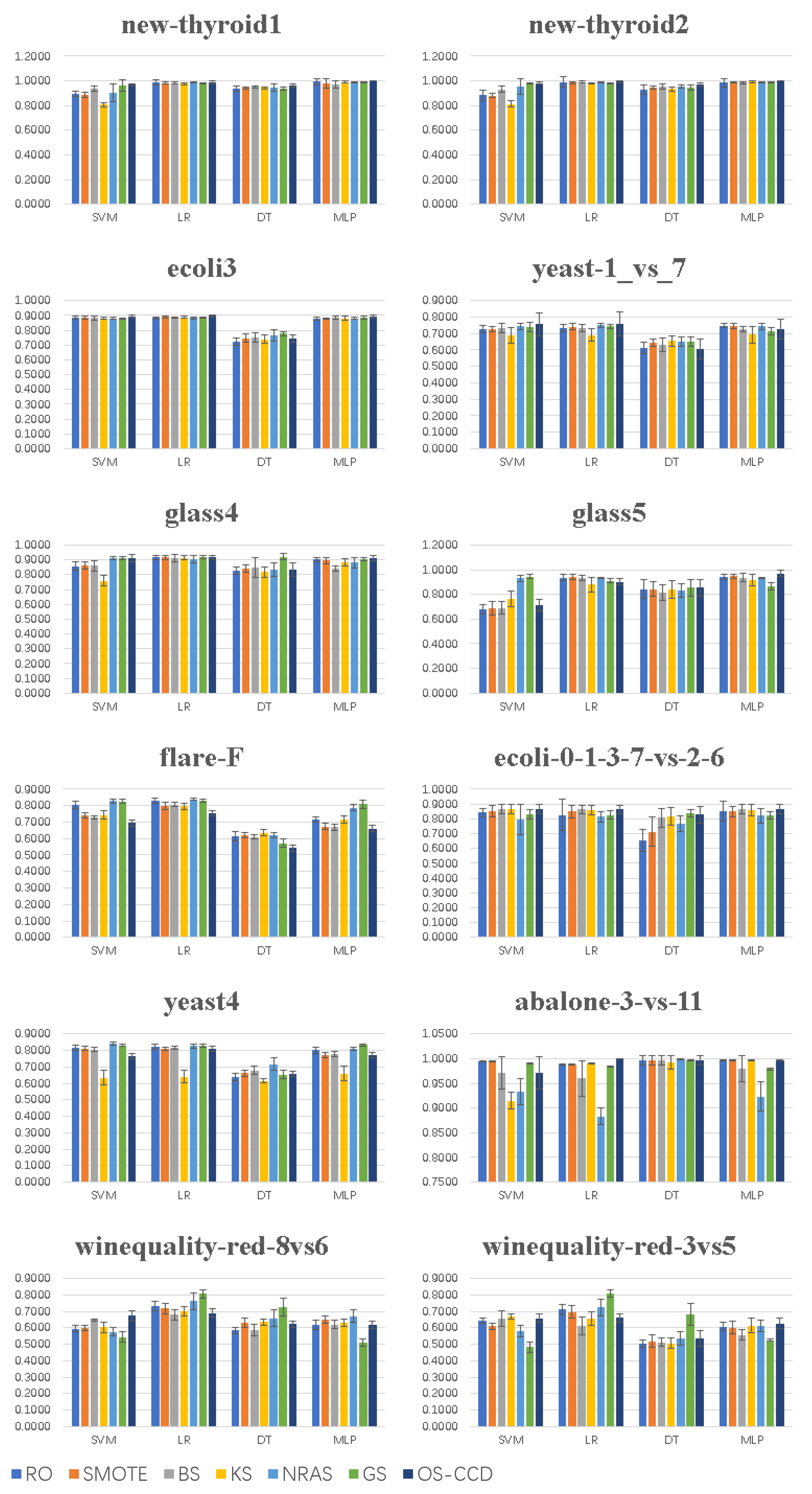
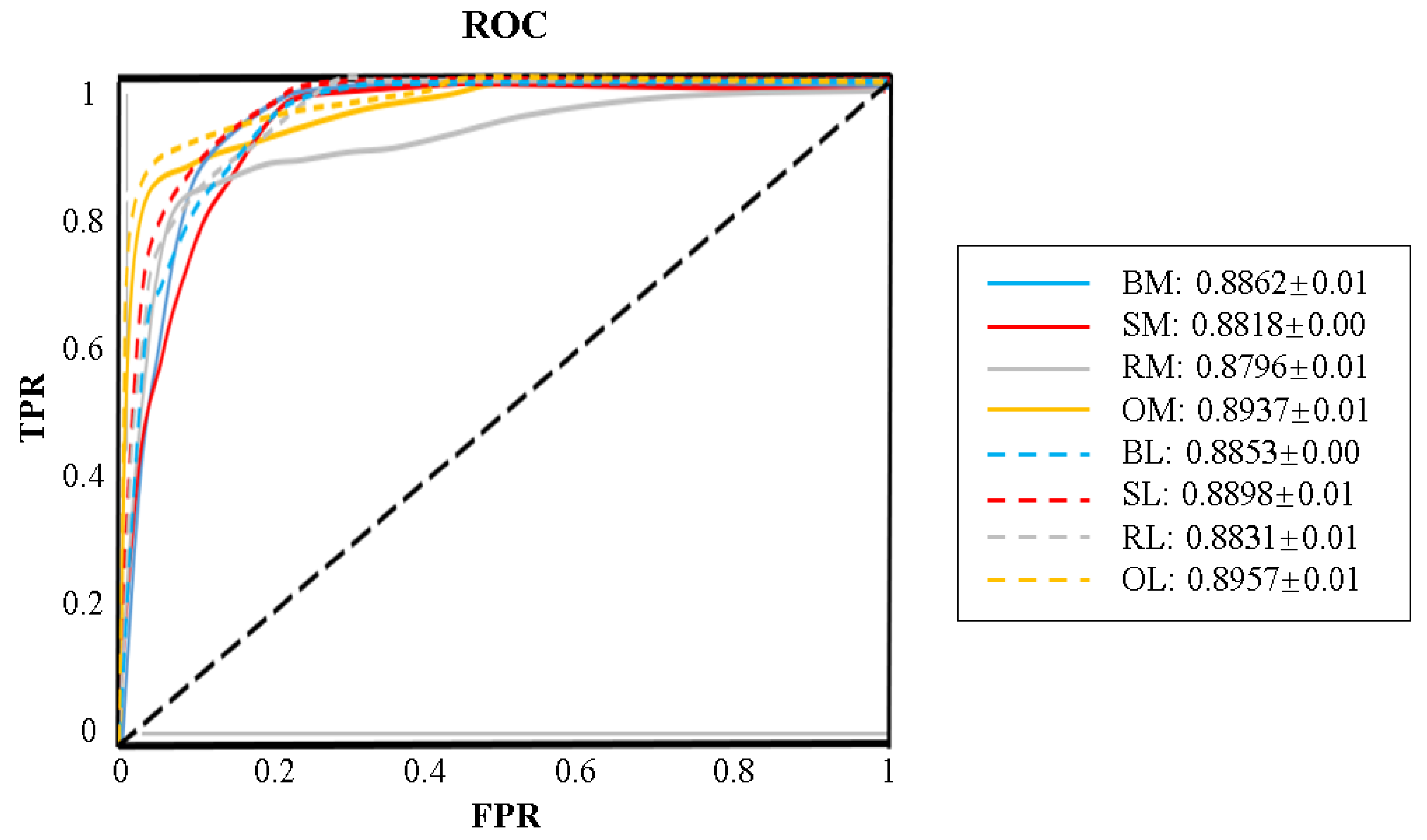
3.3. Experimental Results
4. Conclusions
Author Contributions
Funding
Data Availability Statement
Conflicts of Interest
References
- Kovács, G. Smote-variants: A python implementation of 85 minority oversampling techniques. Neurocomputing 2019, 366, 352–354. [Google Scholar] [CrossRef]
- Kovács, G. An empirical comparison and evaluation of minority oversampling techniques on a large number of imbalanced datasets. Appl. Soft Comput. 2019, 83, 105662. [Google Scholar] [CrossRef]
- Brown, I.; Mues, C. An experimental comparison of classification algorithms for imbalanced credit scoring datasets. Expert Syst. Appl. 2012, 39, 3446–3453. [Google Scholar] [CrossRef]
- Samanta, B.; Al-Balushi, K.R.; Al-Araimi, S.A. Artificial neural networks and support vector machines with genetic algorithm for bearing fault detection. Eng. Appl. Artif. Intell. 2003, 16, 657–665. [Google Scholar] [CrossRef]
- Xie, S.; Zhang, X.; Cai, J. Video crowd detection and abnormal behavior model detection based on machine learning method. Neural. Comput. Appl. 2019, 31, 175–184. [Google Scholar] [CrossRef]
- Kalwa, U.; Legner, C.; Kong, T.; Pandey, S. Skin cancer diagnostics with an all-inclusive smartphone application. Symmetry 2019, 11, 790. [Google Scholar] [CrossRef]
- Le, T.; Baik, S.W. A robust framework for self-care problem identification for children with disability. Symmetry 2019, 11, 89. [Google Scholar] [CrossRef]
- Kang, Q.; Fan, Q.W.; Zurada, J.M. Deterministic convergence analysis via smoothing group Lasso regularization and adaptive momentum for Sigma-Pi Sigma neural network. Inf. Sci. 2021, 553, 66–82. [Google Scholar] [CrossRef]
- Díaz-Uriarte, R.; De Andres, S.A. Gene selection and classification of microarray data using random forest. BMC Bioinform. 2006, 7, 3. [Google Scholar] [CrossRef]
- Wang, C.; Deng, C.; Wang, S. Imbalance-XGBoost: Leveraging weighted and focal losses for binary label-imbalanced classification with XGBoost. Pattern Recognit. Lett. 2020, 136, 190–197. [Google Scholar] [CrossRef]
- Thanathamathee, P.; Lursinsap, C. Handling imbalanced datasets with synthetic boundary data generation using bootstrap re-sampling and AdaBoost techniques. Pattern Recognit. Lett. 2013, 34, 1339–1347. [Google Scholar] [CrossRef]
- Kvamme, H.; Sellereite, N.; Aas, K.; Sjursen, S. Predicting mortgage default using convolutional neural networks. Expert Syst. Appl. 2018, 102, 207–217. [Google Scholar] [CrossRef]
- Yu, L.; Zhou, R.; Tang, L.; Chen, R. A DBN-based resampling SVM ensemble learning paradigm for credit classification with imbalanced data. Appl. Soft Comput. 2018, 69, 192–202. [Google Scholar] [CrossRef]
- Elreedy, D.; Atiya, A.F. A comprehensive analysis of synthetic minority oversampling technique (SMOTE) for handling class imbalance. Inf. Sci. 2019, 505, 32–64. [Google Scholar] [CrossRef]
- Bejjanki, K.K.; Gyani, J.; Gugulothu, N. Class Imbalance Reduction (CIR): A Novel Approach to Software Defect Prediction in the Presence of Class Imbalance. Symmetry 2020, 12, 407. [Google Scholar] [CrossRef]
- Mulyanto, M.; Faisal, M.; Prakosa, S.W.; Leu, J.-S. Effectiveness of Focal Loss for Minority Classification in Network Intrusion Detection Systems. Symmetry 2021, 13, 4. [Google Scholar] [CrossRef]
- Hao, W.; Liu, F. Imbalanced Data Fault Diagnosis Based on an Evolutionary Online Sequential Extreme Learning Machine. Symmetry 2020, 12, 1204. [Google Scholar] [CrossRef]
- Chawla, N.V.; Bowyer, K.W.; Hall, L.O.; Kegelmeyer, W.P. SMOTE: Synthetic minority over-sampling technique. J. Artif. Intell. Res. 2002, 16, 321–357. [Google Scholar] [CrossRef]
- Soltanzadeh, P.; Hashemzadeh, M. RCSMOTE: Range-Controlled synthetic minority over-sampling technique for handling the class imbalance problem. Inf. Sci. 2020, 542, 92–111. [Google Scholar] [CrossRef]
- Han, H.; Wang, W.Y.; Mao, B.H. Borderline-SMOTE: A new over-sampling method in imbalanced datasets learning. In Proceedings of the International Conference on Intelligent Computing (ICIC), Hefei, China, 23–26 August 2005; pp. 878–887. [Google Scholar]
- Douzas, G.; Bacao, F.; Last, F. Improving imbalanced learning through a heuristic oversampling method based on k-means and SMOTE. Inf. Sci. 2018, 465, 1–20. [Google Scholar] [CrossRef]
- Douzas, G.; Bacao, F. Geometric SMOTE a geometrically enhanced drop-in replacement for SMOTE. Inf. Sci. 2019, 501, 118–135. [Google Scholar] [CrossRef]
- Maciejewski, T.; Stefanowski, J. Local neighbourhood extension of SMOTE for mining imbalanced data. In Proceedings of the IEEE Symposium on Computational Intelligence and Data Mining (CIDM), Paris, France, 11–15 April 2011; pp. 104–111. [Google Scholar]
- Bunkhumpornpat, C.; Sinapiromsaran, K.; Lursinsap, C. DBSMOTE: Density-based synthetic minority over-sampling technique. Appl. Intell. 2012, 36, 664–684. [Google Scholar] [CrossRef]
- Maldonado, S.; López, J.; Vairetti, C. An alternative SMOTE oversampling strategy for high-dimensional datasets. Appl. Soft Comput. 2019, 76, 380–389. [Google Scholar] [CrossRef]
- Pan, T.; Zhao, J.; Wu, W.; Yang, J. Learning imbalanced datasets based on SMOTE and Gaussian distribution. Inf. Sci. 2020, 512, 1214–1233. [Google Scholar] [CrossRef]
- He, H.; Bai, Y.; Garcia, E.A.; Li, S. ADASYN: Adaptive synthetic sampling approach for imbalanced learning. In Proceedings of the IEEE International Joint Conference on Neural Networks (IJCNN), Hong Kong, China, 1–8 June 2008; pp. 1322–1328. [Google Scholar]
- Fernández, A.; Garcia, S.; Herrera, F.; Chawla, N.V. SMOTE for learning from imbalanced data: Progress and challenges, marking the 15-year anniversary. J. Artif. Intell. Res. 2018, 61, 863–905. [Google Scholar] [CrossRef]
- Alcalá-Fdez, J.; Fernández, A.; Luengo, J.; Derrac, J.; García, S.; Sánchez, L.; Herrera, F. Keel data-mining software tool: Data set repository, integration of algorithms and experimental analysis framework. J. Mult-Valued Log. Soft Comput. 2011, 17, 255–287. [Google Scholar]
- Huang, J.; Ling, C.X. Using AUC and accuracy in evaluating learning algorithms. IEEE Trans. Knowl. Data Eng. 2005, 17, 299–310. [Google Scholar] [CrossRef]
- Al-Azani, S.; El-Alfy, E.S.M. Using Word Embedding and Ensemble Learning for Highly Imbalanced Data Sentiment Analysis in Short Arabic Text. In Proceedings of the International Conference on Ambient Systems, Networks and Technologies and International Conference on Sustainable Energy Information Technology (ANT/SEIT), Madeira, Portugal, 16–19 May 2017; pp. 359–366. [Google Scholar]
- Liu, A.; Ghosh, J.; Martin, C.E. Generative Oversampling for Mining Imbalanced Datasets. In Proceedings of the International Conference on Data Mining (DMIN), Las Vegas, NV, USA, 25–28 June 2007; pp. 66–72. [Google Scholar]
- Rivera, W.A. Noise reduction a priori synthetic over-sampling for class imbalanced datasets. Inf. Sci. 2017, 408, 146–161. [Google Scholar] [CrossRef]
- Lee, H.; Kim, J.; Kim, S. Gaussian-Based SMOTE Algorithm for Solving Skewed Class Distributions. Int. J. Fuzzy Log. Intell. Syst. 2017, 17, 229–234. [Google Scholar] [CrossRef]
- Kang, Q.; Shi, L.; Zhou, M.; Wang, X.; Wu, Q.; Wei, Z. A distance-based weighted undersampling scheme for support vector machines and its application to imbalanced classification. IEEE Trans. Neural Netw. Learn. Syst. 2017, 29, 4152–4165. [Google Scholar] [CrossRef]
- Nie, G.; Rowe, W.; Zhang, L.; Tian, Y.; Shi, Y. Credit card churn forecasting by logistic regression and decision tree. Expert Syst. Appl. 2011, 38, 15273–15285. [Google Scholar] [CrossRef]
- Oh, S.H. Error back-propagation algorithm for classification of imbalanced data. Neurocomputing 2011, 74, 1058–1061. [Google Scholar] [CrossRef]
- Wold, S.; Esbensen, K.; Geladi, P. Principal component analysis. Chemom. Intell. Lab. Syst. 1987, 2, 37–52. [Google Scholar] [CrossRef]


| ID | Dataset | Positive | Negative | Attribute | IR |
|---|---|---|---|---|---|
| 1 | new-thyroid1 | 35 | 180 | 5 | 5.14 |
| 2 | new-thyroid2 | 35 | 180 | 5 | 5.14 |
| 3 | ecoli3 | 35 | 301 | 7 | 8.6 |
| 4 | yeast-1_vs_7 | 30 | 429 | 7 | 14.3 |
| 5 | glass4 | 13 | 201 | 9 | 15.46 |
| 6 | glass5 | 9 | 205 | 9 | 22.78 |
| 7 | flare-F | 43 | 1023 | 11 | 23.79 |
| 8 | ecoli-0-1-3-7-vs-2-6 | 7 | 190 | 7 | 27.14 |
| 9 | yeast4 | 51 | 1433 | 8 | 28.1 |
| 10 | abalone-3-vs-11 | 15 | 487 | 8 | 32.47 |
| 11 | winequality-red-8vs6 | 18 | 638 | 11 | 35.44 |
| 12 | winequality-red-3vs5 | 10 | 681 | 11 | 68.1 |
| Group | Group | ||
|---|---|---|---|
| SVM | RS: Random oversampling + SVM | DT | RD: Random oversampling + DT |
| SS: SMOTE + SVM | SD: SMOTE + DT | ||
| BS: Borderline-SMOTE + SVM | BD: BorderlineSMOTE + DT | ||
| KMS: k-meas-SMOTE + SVM | KMD: k-meas-SMOTE + DT | ||
| NS: NRAS + SVM | ND: NRAS + DT | ||
| GS: Gaussian-SMOTE + SVM | GD: Gaussian-SMOTE + DT | ||
| OS: OS-CCD + SVM | OD: OS-CCD + DT | ||
| LR | RL: Random oversampling + LR | MLP | RM:Random oversampling + MLP |
| SL: SMOTE + LR | SM: SMOTE + MLP | ||
| BL: Borderline-SMOTE + LR | BM: Borderline-SMOTE + MLP | ||
| KML: k-means-SMOTE + LR | KMM: k-meas-SMOTE + MLP | ||
| NL: NRAS + LR | NM: NRAS + MLP | ||
| GL: Gaussian-SMOTE + LR | GM: Gaussian-SMOTE + MLP | ||
| OL: OS-CCD + LR | OM: OS-CCD + MLP |
| RO | SMOTE | BS | KS | NRAS | GS | OS-CCD | ||
|---|---|---|---|---|---|---|---|---|
| 1 | SVM | 0.9586 ± 0.01 | 0.9540 ± 0.01 | 0.9107 ± 0.02 | 0.9256 ± 0.01 | 0.9563 ± 0.02 | 0.9349 ± 0.08 | 0.9619 ± 0.01 |
| LR | 0.9884 ± 0.00 | 0.9870 ± 0.00 | 0.9856 ± 0.00 | 0.9874 ± 0.00 | 0.9823 ± 0.00 | 0.9660 ± 0.01 | 0.9856 ± 0.00 | |
| DT | 0.9693 ± 0.01 | 0.9730 ± 0.01 | 0.9740 ± 0.01 | 0.9702 ± 0.01 | 0.9577 ± 0.02 | 0.9381 ± 0.01 | 0.9805 ± 0.00 | |
| MLP | 0.9888 ± 0.00 | 0.9647 ± 0.06 | 0.9670 ± 0.01 | 0.9940 ± 0.00 | 0.9833 ± 0.00 | 0.9879 ± 0.00 | 0.9953 ± 0.00 | |
| 2 | SVM | 0.9544 ± 0.02 | 0.9502 ± 0.01 | 0.9079 ± 0.02 | 0.9256 ± 0.01 | 0.9693 ± 0.02 | 0.9716 ± 0.00 | 0.9865 ± 0.00 |
| LR | 0.9921 ± 0.01 | 0.9898 ± 0.00 | 0.9893 ± 0.00 | 0.9893 ± 0.00 | 0.9795 ± 0.00 | 0.9670 ± 0.01 | 0.9907 ± 0.00 | |
| DT | 0.9651 ± 0.01 | 0.9712 ± 0.01 | 0.9735 ± 0.01 | 0.9674 ± 0.01 | 0.9619 ± 0.01 | 0.9493 ± 0.01 | 0.9819 ± 0.01 | |
| MLP | 0.9791 ± 0.01 | 0.9819 ± 0.01 | 0.9740 ± 0.01 | 0.9944 ± 0.00 | 0.9795 ± 0.00 | 0.9865 ± 0.00 | 0.9953 ± 0.00 | |
| 3 | SVM | 0.8836 ± 0.01 | 0.8962 ± 0.01 | 0.8944 ± 0.01 | 0.9015 ± 0.01 | 0.8506 ± 0.00 | 0.8229 ± 0.00 | 0.9155 ± 0.01 |
| LR | 0.8516 ± 0.01 | 0.8614 ± 0.00 | 0.8397 ± 0.00 | 0.8569 ± 0.01 | 0.8515 ± 0.00 | 0.8345 ± 0.01 | 0.8697 ± 0.01 | |
| DT | 0.9045 ± 0.01 | 0.8888 ± 0.01 | 0.8982 ± 0.01 | 0.8980 ± 0.01 | 0.8822 ± 0.01 | 0.9108 ± 0.01 | 0.9016 ± 0.01 | |
| MLP | 0.8703 ± 0.01 | 0.8786 ± 0.00 | 0.8617 ± 0.01 | 0.8768 ± 0.02 | 0.8747 ± 0.01 | 0.8646 ± 0.00 | 0.9158 ± 0.00 | |
| 4 | SVM | 0.7865 ± 0.01 | 0.7834 ± 0.01 | 0.8342 ± 0.01 | 0.8312 ± 0.03 | 0.7273 ± 0.01 | 0.8020 ± 0.01 | 0.7983 ± 0.03 |
| LR | 0.7575 ± 0.01 | 0.7580 ± 0.01 | 0.7787 ± 0.01 | 0.7715 ± 0.04 | 0.7380 ± 0.01 | 0.7608 ± 0.01 | 0.8290 ± 0.02 | |
| DT | 0.9026 ± 0.02 | 0.8830 ± 0.01 | 0.8922 ± 0.01 | 0.8996 ± 0.01 | 0.8460 ± 0.01 | 0.9041 ± 0.01 | 0.8523 ± 0.03 | |
| MLP | 0.7900 ± 0.01 | 0.8002 ± 0.01 | 0.8272 ± 0.01 | 0.7867 ± 0.02 | 0.7528 ± 0.01 | 0.7360 ± 0.02 | 0.8314 ± 0.02 | |
| 5 | SVM | 0.8495 ± 0.01 | 0.8430 ± 0.01 | 0.8458 ± 0.02 | 0.7636 ± 0.06 | 0.9047 ± 0.01 | 0.9108 ± 0.00 | 0.9350 ± 0.01 |
| LR | 0.9243 ± 0.00 | 0.9238 ± 0.01 | 0.9257 ± 0.01 | 0.9257 ± 0.00 | 0.9000 ± 0.01 | 0.9160 ± 0.01 | 0.9262 ± 0.01 | |
| DT | 0.9575 ± 0.01 | 0.9613 ± 0.01 | 0.9631 ± 0.01 | 0.9575 ± 0.01 | 0.9261 ± 0.01 | 0.9181 ± 0.01 | 0.9575 ± 0.01 | |
| MLP | 0.8991 ± 0.01 | 0.9010 ± 0.01 | 0.8987 ± 0.01 | 0.9178 ± 0.01 | 0.8693 ± 0.01 | 0.8945 ± 0.01 | 0.9565 ± 0.01 | |
| 6 | SVM | 0.8184 ± 0.01 | 0.8020 ± 0.01 | 0.7937 ± 0.01 | 0.6788 ± 0.08 | 0.8916 ± 0.01 | 0.9042 ± 0.01 | 0.7963 ± 0.01 |
| LR | 0.9039 ± 0.01 | 0.9071 ± 0.01 | 0.8978 ± 0.01 | 0.8791 ± 0.01 | 0.8705 ± 0.01 | 0.8344 ± 0.01 | 0.9337 ± 0.01 | |
| DT | 0.9818 ± 0.01 | 0.9785 ± 0.00 | 0.9771 ± 0.01 | 0.9739 ± 0.01 | 0.9305 ± 0.02 | 0.9389 ± 0.02 | 0.9799 ± 0.01 | |
| MLP | 0.9029 ± 0.01 | 0.9057 ± 0.01 | 0.8968 ± 0.01 | 0.9132 ± 0.02 | 0.8780 ± 0.01 | 0.8154 ± 0.02 | 0.9865 ± 0.00 | |
| 7 | SVM | 0.8417 ± 0.01 | 0.8457 ± 0.01 | 0.8584 ± 0.01 | 0.8596 ± 0.01 | 0.8102 ± 0.01 | 0.8178 ± 0.00 | 0.9250 ± 0.01 |
| LR | 0.8400 ± 0.00 | 0.8280 ± 0.00 | 0.8369 ± 0.01 | 0.8492 ± 0.01 | 0.8305 ± 0.00 | 0.8255 ± 0.00 | 0.9015 ± 0.01 | |
| DT | 0.8932 ± 0.01 | 0.9050 ± 0.00 | 0.9171 ± 0.00 | 0.9057 ± 0.01 | 0.8913 ± 0.01 | 0.9461 ± 0.00 | 0.9406 ± 0.00 | |
| MLP | 0.8801 ± 0.01 | 0.8899 ± 0.01 | 0.9084 ± 0.01 | 0.8806 ± 0.01 | 0.8572 ± 0.01 | 0.8502 ± 0.01 | 0.9313 ± 0.00 | |
| 8 | SVM | 0.9490 ± 0.02 | 0.9764 ± 0.01 | 0.9918 ± 0.00 | 0.9907 ± 0.00 | 0.9149 ± 0.02 | 0.9656 ± 0.01 | 0.9918 ± 0.00 |
| LR | 0.9488 ± 0.02 | 0.9532 ± 0.01 | 0.9896 ± 0.00 | 0.9863 ± 0.00 | 0.9151 ± 0.01 | 0.9560 ± 0.01 | 0.9896 ± 0.00 | |
| DT | 0.9742 ± 0.01 | 0.9742 ± 0.01 | 0.9784 ± 0.00 | 0.9786 ± 0.00 | 0.9630 ± 0.01 | 0.9825 ± 0.00 | 0.9784 ± 0.00 | |
| MLP | 0.9775 ± 0.01 | 0.9827 ± 0.01 | 0.9899 ± 0.00 | 0.9899 ± 0.00 | 0.9497 ± 0.01 | 0.9505 ± 0.01 | 0.9912 ± 0.00 | |
| 9 | SVM | 0.8664 ± 0.00 | 0.8775 ± 0.01 | 0.9158 ± 0.00 | 0.8685 ± 0.01 | 0.8557 ± 0.00 | 0.8562 ± 0.00 | 0.9348 ± 0.00 |
| LR | 0.8550 ± 0.00 | 0.8560 ± 0.00 | 0.8922 ± 0.00 | 0.8161 ± 0.01 | 0.8483 ± 0.00 | 0.8472 ± 0.00 | 0.9013 ± 0.01 | |
| DT | 0.9549 ± 0.00 | 0.9375 ± 0.00 | 0.9424 ± 0.00 | 0.9398 ± 0.01 | 0.9268 ± 0.01 | 0.9474 ± 0.00 | 0.9459 ± 0.00 | |
| MLP | 0.8842 ± 0.01 | 0.8862 ± 0.01 | 0.9139 ± 0.01 | 0.8642 ± 0.01 | 0.8381 ± 0.01 | 0.8575 ± 0.00 | 0.9282 ± 0.00 | |
| 10 | SVM | 0.9906 ± 0.00 | 0.9914 ± 0.00 | 0.9942 ± 0.00 | 0.9906 ± 0.00 | 0.9956 ± 0.00 | 0.9811 ± 0.00 | 0.9954 ± 0.00 |
| LR | 0.9759 ± 0.00 | 0.9763 ± 0.00 | 0.9783 ± 0.00 | 0.9823 ± 0.00 | 0.9930 ± 0.00 | 0.9675 ± 0.00 | 1.0000 ± 0.00 | |
| DT | 0.9990 ± 0.00 | 0.9994 ± 0.00 | 0.9992 ± 0.00 | 0.9990 ± 0.00 | 0.9990 ± 0.00 | 0.9934 ± 0.00 | 0.9996 ± 0.00 | |
| MLP | 0.9930 ± 0.00 | 0.9938 ± 0.00 | 0.9918 ± 0.00 | 0.9934 ± 0.00 | 0.9944 ± 0.00 | 0.9588 ± 0.00 | 0.9946 ± 0.00 | |
| 11 | SVM | 0.6635 ± 0.01 | 0.6547 ± 0.01 | 0.7880 ± 0.00 | 0.7176 ± 0.03 | 0.8265 ± 0.01 | 0.8081 ± 0.01 | 0.8944 ± 0.04 |
| LR | 0.8030 ± 0.00 | 0.8122 ± 0.00 | 0.8799 ± 0.01 | 0.8532 ± 0.01 | 0.7669 ± 0.01 | 0.7759 ± 0.00 | 0.8976 ± 0.01 | |
| DT | 0.9570 ± 0.00 | 0.9459 ± 0.01 | 0.9534 ± 0.00 | 0.9524 ± 0.01 | 0.9110 ± 0.01 | 0.8738 ± 0.02 | 0.9540 ± 0.01 | |
| MLP | 0.8596 ± 0.01 | 0.8634 ± 0.01 | 0.9364 ± 0.01 | 0.8947 ± 0.01 | 0.7959 ± 0.03 | 0.8850 ± 0.01 | 0.9453 ± 0.00 | |
| 12 | SVM | 0.6833 ± 0.03 | 0.5773 ± 0.02 | 0.9042 ± 0.01 | 0.8185 ± 0.04 | 0.8774 ± 0.01 | 0.8237 ± 0.01 | 0.9632 ± 0.01 |
| LR | 0.8577 ± 0.01 | 0.8674 ± 0.01 | 0.9562 ± 0.01 | 0.9226 ± 0.01 | 0.7970 ± 0.01 | 0.8348 ± 0.01 | 0.9514 ± 0.01 | |
| DT | 0.9715 ± 0.00 | 0.9528 ± 0.01 | 0.9667 ± 0.00 | 0.9669 ± 0.00 | 0.9449 ± 0.01 | 0.9211 ± 0.01 | 0.9695 ± 0.00 | |
| MLP | 0.9431 ± 0.01 | 0.9109 ± 0.01 | 0.9695 ± 0.00 | 0.9473 ± 0.01 | 0.8765 ± 0.01 | 0.9375 ± 0.01 | 0.9699 ± 0.00 |
| RO | SMOTE | BS | KS | NRAS | GS | OS-CCD | ||
|---|---|---|---|---|---|---|---|---|
| 1 | SVM | 0.8594 ± 0.02 | 0.8439 ± 0.02 | 0.7949 ± 0.04 | 0.7211 ± 0.03 | 0.8440 ± 0.09 | 0.8624 ± 0.13 | 0.8999 ± 0.02 |
| LR | 0.9656 ± 0.01 | 0.9608 ± 0.01 | 0.9584 ± 0.01 | 0.9606 ± 0.01 | 0.9515 ± 0.01 | 0.9101 ± 0.02 | 0.9593 ± 0.01 | |
| DT | 0.9016 ± 0.02 | 0.9143 ± 0.02 | 0.9201 ± 0.02 | 0.9068 ± 0.02 | 0.8794 ± 0.05 | 0.8353 ± 0.02 | 0.9392 ± 0.01 | |
| MLP | 0.9685 ± 0.01 | 0.9350 ± 0.06 | 0.9010 ± 0.05 | 0.9818 ± 0.01 | 0.9541 ± 0.01 | 0.9662 ± 0.01 | 0.9867 ± 0.00 | |
| 2 | SVM | 0.8422 ± 0.06 | 0.8310 ± 0.03 | 0.7827 ± 0.05 | 0.7287 ± 0.04 | 0.9025 ± 0.08 | 0.9237 ± 0.01 | 0.9599 ± 0.01 |
| LR | 0.9767 ± 0.05 | 0.9690 ± 0.01 | 0.9690 ± 0.01 | 0.9664 ± 0.01 | 0.9445 ± 0.01 | 0.9139 ± 0.01 | 0.9729 ± 0.01 | |
| DT | 0.8890 ± 0.05 | 0.9090 ± 0.02 | 0.9200 ± 0.03 | 0.8966 ± 0.02 | 0.8923 ± 0.02 | 0.8620 ± 0.03 | 0.9467 ± 0.02 | |
| MLP | 0.9418 ± 0.04 | 0.9498 ± 0.01 | 0.9306 ± 0.02 | 0.9834 ± 0.01 | 0.9444 ± 0.01 | 0.9621 ± 0.01 | 0.9867 ± 0.00 | |
| 3 | SVM | 0.6179 ± 0.01 | 0.6395 ± 0.02 | 0.6363 ± 0.02 | 0.6481 ± 0.02 | 0.5691 ± 0.01 | 0.5315 ± 0.01 | 0.6856 ± 0.03 |
| LR | 0.5725 ± 0.01 | 0.5900 ± 0.01 | 0.5622 ± 0.01 | 0.5874 ± 0.02 | 0.5727 ± 0.01 | 0.5507 ± 0.01 | 0.6060 ± 0.01 | |
| DT | 0.5147 ± 0.04 | 0.5122 ± 0.04 | 0.5339 ± 0.05 | 0.5206 ± 0.05 | 0.5232 ± 0.05 | 0.5832 ± 0.03 | 0.5373 ± 0.04 | |
| MLP | 0.5943 ± 0.01 | 0.6093 ± 0.01 | 0.5900 ± 0.02 | 0.6129 ± 0.02 | 0.6040 ± 0.02 | 0.5981 ± 0.01 | 0.6870 ± 0.01 | |
| 4 | SVM | 0.2835 ± 0.02 | 0.2815 ± 0.01 | 0.3269 ± 0.04 | 0.2893 ± 0.05 | 0.2714 ± 0.02 | 0.3078 ± 0.02 | 0.3126 ± 0.05 |
| LR | 0.2727 ± 0.02 | 0.2779 ± 0.01 | 0.2853 ± 0.02 | 0.2498 ± 0.03 | 0.2785 ± 0.01 | 0.2861 ± 0.01 | 0.3392 ± 0.05 | |
| DT | 0.2743 ± 0.08 | 0.2869 ± 0.04 | 0.2783 ± 0.06 | 0.3212 ± 0.05 | 0.2633 ± 0.03 | 0.3256 ± 0.06 | 0.2256 ± 0.04 | |
| MLP | 0.3013 ± 0.01 | 0.3087 ± 0.01 | 0.3147 ± 0.02 | 0.2573 ± 0.04 | 0.2838 ± 0.02 | 0.2556 ± 0.01 | 0.3154 ± 0.04 | |
| 5 | SVM | 0.4206 ± 0.03 | 0.4075 ± 0.04 | 0.4097 ± 0.04 | 0.2900 ± 0.05 | 0.5532 ± 0.02 | 0.5665 ± 0.03 | 0.6274 ± 0.06 |
| LR | 0.5968 ± 0.03 | 0.5952 ± 0.03 | 0.5957 ± 0.04 | 0.5972 ± 0.02 | 0.5384 ± 0.04 | 0.5872 ± 0.03 | 0.6032 ± 0.03 | |
| DT | 0.6493 ± 0.06 | 0.6858 ± 0.07 | 0.6816 ± 0.11 | 0.6391 ± 0.08 | 0.5576 ± 0.08 | 0.6160 ± 0.04 | 0.6621 ± 0.07 | |
| MLP | 0.5287 ± 0.03 | 0.5336 ± 0.04 | 0.4819 ± 0.03 | 0.5637 ± 0.04 | 0.4812 ± 0.06 | 0.5307 ± 0.03 | 0.7198 ± 0.04 | |
| 6 | SVM | 0.1903 ± 0.04 | 0.1872 ± 0.04 | 0.1926 ± 0.03 | 0.2009 ± 0.03 | 0.4501 ± 0.04 | 0.4847 ± 0.02 | 0.2041 ± 0.02 |
| LR | 0.4891 ± 0.05 | 0.5014 ± 0.04 | 0.4734 ± 0.03 | 0.3753 ± 0.05 | 0.4086 ± 0.02 | 0.3522 ± 0.03 | 0.5694 ± 0.07 | |
| DT | 0.6808 ± 0.13 | 0.6748 ± 0.10 | 0.6414 ± 0.11 | 0.6709 ± 0.12 | 0.4947 ± 0.11 | 0.5245 ± 0.10 | 0.7048 ± 0.12 | |
| MLP | 0.4966 ± 0.04 | 0.5042 ± 0.03 | 0.4840 ± 0.06 | 0.5064 ± 0.08 | 0.4210 ± 0.02 | 0.3055 ± 0.03 | 0.8734 ± 0.04 | |
| 7 | SVM | 0.2821 ± 0.01 | 0.2491 ± 0.02 | 0.2514 ± 0.01 | 0.2676 ± 0.02 | 0.2673 ± 0.01 | 0.2712 ± 0.01 | 0.3262 ± 0.02 |
| LR | 0.2942 ± 0.01 | 0.2655 ± 0.01 | 0.2790 ± 0.01 | 0.2875 ± 0.02 | 0.2894 ± 0.00 | 0.2804 ± 0.01 | 0.3266 ± 0.02 | |
| DT | 0.1894 ± 0.03 | 0.2088 ± 0.02 | 0.2088 ± 0.02 | 0.2251 ± 0.02 | 0.1951 ± 0.02 | 0.1842 ± 0.05 | 0.1184 ± 0.03 | |
| MLP | 0.2659 ± 0.02 | 0.2455 ± 0.03 | 0.2660 ± 0.02 | 0.2688 ± 0.02 | 0.2883 ± 0.02 | 0.2943 ± 0.01 | 0.3012 ± 0.03 | |
| 8 | SVM | 0.3562 ± 0.11 | 0.5282 ± 0.11 | 0.7233 ± 0.07 | 0.7027 ± 0.08 | 0.1981 ± 0.07 | 0.4116 ± 0.10 | 0.7233 ± 0.07 |
| LR | 0.3286 ± 0.09 | 0.3621 ± 0.07 | 0.6880 ± 0.06 | 0.6427 ± 0.07 | 0.2273 ± 0.04 | 0.3596 ± 0.07 | 0.6880 ± 0.06 | |
| DT | 0.2904 ± 0.10 | 0.3580 ± 0.15 | 0.4901 ± 0.11 | 0.5154 ± 0.12 | 0.3658 ± 0.09 | 0.5670 ± 0.07 | 0.5305 ± 0.10 | |
| MLP | 0.5448 ± 0.12 | 0.5817 ± 0.12 | 0.7000 ± 0.07 | 0.6967 ± 0.07 | 0.3389 ± 0.10 | 0.3259 ± 0.05 | 0.7133 ± 0.06 | |
| 9 | SVM | 0.2848 ± 0.01 | 0.2967 ± 0.02 | 0.3584 ± 0.01 | 0.1684 ± 0.03 | 0.2839 ± 0.01 | 0.2797 ± 0.01 | 0.3806 ± 0.03 |
| LR | 0.2738 ± 0.01 | 0.2671 ± 0.01 | 0.3205 ± 0.01 | 0.1477 ± 0.02 | 0.2681 ± 0.01 | 0.2687 ± 0.01 | 0.3330 ± 0.01 | |
| DT | 0.3107 ± 0.05 | 0.2799 ± 0.03 | 0.3173 ± 0.04 | 0.2298 ± 0.03 | 0.3123 ± 0.04 | 0.3049 ± 0.04 | 0.2958 ± 0.03 | |
| MLP | 0.2977 ± 0.02 | 0.2830 ± 0.01 | 0.3364 ± 0.02 | 0.1828 ± 0.03 | 0.2513 ± 0.01 | 0.2829 ± 0.01 | 0.3630 ± 0.01 | |
| 10 | SVM | 0.8790 ± 0.01 | 0.8881 ± 0.02 | 0.9014 ± 0.04 | 0.8328 ± 0.04 | 0.9033 ± 0.05 | 0.7823 ± 0.02 | 0.9171 ± 0.05 |
| LR | 0.7330 ± 0.02 | 0.7357 ± 0.02 | 0.7200 ± 0.05 | 0.7871 ± 0.03 | 0.8460 ± 0.03 | 0.6725 ± 0.01 | 1.0000 ± 0.00 | |
| DT | 0.9846 ± 0.02 | 0.9903 ± 0.02 | 0.9874 ± 0.02 | 0.9836 ± 0.02 | 0.9857 ± 0.01 | 0.9119 ± 0.03 | 0.9931 ± 0.01 | |
| MLP | 0.9069 ± 0.011 | 0.9176 ± 0.02 | 0.8812 ± 0.04 | 0.9139 ± 0.02 | 0.8931 ± 0.05 | 0.6155 ± 0.01 | 0.9288 ± 0.02 | |
| 11 | SVM | 0.0781 ± 0.01 | 0.0791 ± 0.01 | 0.1164 ± 0.00 | 0.0919 ± 0.01 | 0.0870 ± 0.01 | 0.0673 ± 0.02 | 0.1909 ± 0.03 |
| LR | 0.1547 ± 0.01 | 0.1510 ± 0.02 | 0.1776 ± 0.03 | 0.1686 ± 0.01 | 0.1497 ± 0.02 | 0.1705 ± 0.01 | 0.1981 ± 0.02 | |
| DT | 0.1844 ± 0.04 | 0.2255 ± 0.04 | 0.1833 ± 0.06 | 0.2573 ± 0.06 | 0.1981 ± 0.05 | 0.2006 ± 0.04 | 0.2313 ± 0.02 | |
| MLP | 0.1316 ± 0.03 | 0.1471 ± 0.02 | 0.2049 ± 0.03 | 0.1637 ± 0.03 | 0.1268 ± 0.02 | 0.0526 ± 0.02 | 0.2174 ± 0.03 | |
| 12 | SVM | 0.0527 ± 0.01 | 0.0376 ± 0.00 | 0.0988 ± 0.02 | 0.0786 ± 0.01 | 0.0538 ± 0.02 | 0.020 ± 0.01 | 0.2136 ± 0.07 |
| LR | 0.0987 ± 0.01 | 0.0977 ± 0.01 | 0.1365 ± 0.06 | 0.1195 ± 0.03 | 0.0826 ± 0.02 | 0.1222 ± 0.01 | 0.1692 ± 0.04 | |
| DT | 0.0130 ± 0.03 | 0.0377 ± 0.04 | 0.0274 ± 0.04 | 0.0248 ± 0.05 | 0.0617 ± 0.05 | 0.1428 ± 0.05 | 0.0607 ± 0.07 | |
| MLP | 0.1196 ± 0.03 | 0.0774 ± 0.03 | 0.0918 ± 0.06 | 0.1295 ± 0.07 | 0.0689 ± 0.02 | 0.0394 ± 0.02 | 0.1982 ± 0.06 |
Publisher’s Note: MDPI stays neutral with regard to jurisdictional claims in published maps and institutional affiliations. |
© 2021 by the authors. Licensee MDPI, Basel, Switzerland. This article is an open access article distributed under the terms and conditions of the Creative Commons Attribution (CC BY) license (http://creativecommons.org/licenses/by/4.0/).
Share and Cite
Jiang, Z.; Pan, T.; Zhang, C.; Yang, J. A New Oversampling Method Based on the Classification Contribution Degree. Symmetry 2021, 13, 194. https://doi.org/10.3390/sym13020194
Jiang Z, Pan T, Zhang C, Yang J. A New Oversampling Method Based on the Classification Contribution Degree. Symmetry. 2021; 13(2):194. https://doi.org/10.3390/sym13020194
Chicago/Turabian StyleJiang, Zhenhao, Tingting Pan, Chao Zhang, and Jie Yang. 2021. "A New Oversampling Method Based on the Classification Contribution Degree" Symmetry 13, no. 2: 194. https://doi.org/10.3390/sym13020194
APA StyleJiang, Z., Pan, T., Zhang, C., & Yang, J. (2021). A New Oversampling Method Based on the Classification Contribution Degree. Symmetry, 13(2), 194. https://doi.org/10.3390/sym13020194