Asymmetrical Property of the Subproportionality of Weighting Function in Prospect Theory: Is It Real and How Can It Be Achieved?

Abstract

An asymmetrical property of the probability weighting function, namely, subproportionality, was derived from observations. Subproportionality can provide a reasonable explanation for accommodating the Allais paradox and, therefore, deserves replication for its high impact. The present study aimed to explore the mechanism of subproportionality by comparing the two completely opposite decision mechanisms: prospect theory and equate-to-differentiate theory. Results revealed that the underlying mechanism supports the prediction of equate-to-differentiate theory but not prospect theory in the diagnostic stimuli condition. Knowledge regarding which intra-dimensional difference between Options A and B is greater, not knowledge regarding which option’s overall prospect value is greater, indeed predicts option preference. Our findings may deepen current understanding on the mechanisms behind the simple risky choice with a single-non-zero outcome. Additionally, these findings will hopefully encourage subsequent researchers to take a fresh look at the Allais paradox.

1. Introduction

Prospect theory, developed by Kahneman and Tversky [1], is widely recognized as the leading descriptive theory of decision making under risk [2,3,4,5]. One strength of the theory is that it attempts to address the Allais common ratio paradox [6,7], namely, subproportionality. The Allais common ratio paradox, also known as the common ratio effect, was used by Allais [6] and Kahneman and Tversky [1] as a counterexample to expected utility (EU) theory’s hypothesis of linearity in probabilities [1,8]. Responses to Allais’ [6] choice problems, which gave rise to the Allais paradox, demonstrated behavior that challenged the expectation–maximization principle [9].

Under prospect theory [1], probability weighting function π(p) and value function v(x) are two core functions. For weighting function, decision weight (π) is derived from numerous preferential choices [10] in which probabilities (p) in decision-making situations are nonlinearly transformed into weights: π(p). The probability weighting function exhibits an asymmetrical property, called subproportionality, in which the ratio of probability weights decreases when both probabilities are scaled down by a common factor (r). Specifically, if the modal choice of (x, p) is similar to (y, pq), then (x, pr) is not preferred to (y, pqr), 0 < p, q, r ≤ 1. The above reasoning can be presented by the following equation: π(p) v(x) = π(pq) v(y) implies π(pr) v(x) ≤ π(pqr) v(y). The property of the subproportionality is seen as asymmetrical. As a common factor was symmetrically multiplied, the modal choice is shifted asymmetrically.

For instance, the property of subproportionality can be derived from subjects’ responses to the two games designed by Kahneman and Tversky [1] (

Table 1. Experimental material in Kahneman and Tversky [1].

Game I without r multiplied
A: (6000, 45%)	B: (3000, 90%)
Game II with r multiplied
C: (6000, 0.1%)	D: (3000, 0.2%)

). That is, the choice proportion of (3000, 90%) is equal to the choice proportion of (6000, 45%), and then the choice proportion of (3000, 0.2%) is lesser than that of (6000, 0.1%).

In Kahneman and Tversky’s [1] study, the resulting choice showed that most people (86%) chose Option B (higher probability with smaller outcome, P_o) in Game I without r multiplied. However, in Game II with r symmetrically multiplied, most people (73%) asymmetrically changed their preference and chose Option C (larger outcome with lower probability, O_p). The so-called subproportionality of decision weight (π) was thus derived from the asymmetrical pattern of preferences observed in Kahneman and Tversky’s study [1].

Subproportionality, as an important property, is needed for prospect theory to explain the Allais common ratio paradox [11,12,13,14] and the subproportionality itself deserves replication. Replication has long been regarded as a central feature of scientific research, and recent debates show that psychologists have rediscovered its importance [15,16]. Further, documented cross-national differences in risk preference are still controversial among American and Asian populations. Therefore, precise replication in China can be an important attempt to confirm an earlier study′s finding. Accumulated studies show that respondents in Asian cultures (e.g., Chinese) are more risk-seeking than respondents in other cultures (e.g., the United States); however, reciprocal predictions are in total opposition [17,18,19,20]. Particularly, most respondents from Singapore, Hong Kong, Macao, and the Chinese mainland [9,21,22] tend to choose Option B (risky) when faced with the first pair of choice problems in the Allais common consequence paradox [6] (The Allais common consequence paradox comprises two pairs of choices, with each pair having two alternative prospects as follows: First pair of choices: A (1 M, 1.0) vs. B (5 M, 0.10; 1 M, 0.89; 0, 0.01); Second pair of choices: C (1 M, 0.11; 0, 0.89) vs. D (5 M, 0.10; 0, 0.90.). Contrastingly, Allais’s choice violated the sure-thing principle and led to the emergence of the Allais paradox.

The failure to replicate the Allais common consequence paradox [6] in Asian cultures creates doubt as to whether subproportionality is sufficiently robust for the Allais common ratio paradox to work in an Asian country, such as China. Thus, we first aimed to investigate the reliability and robustness of Kahneman and Tversky’s [1] findings by conducting a straightforward replication study.

To date, at least two completely opposite mechanisms have been identified (i.e., compensatory and holistic vs. non-compensatory and dimensional) that can explain what makes subproportionality work. To illustrate this, we used prospect theory [1,23] and equate-to-differentiate theory [24,25,26,27] as each mechanism’s representative.

1.1. Prospect Theory

Guided by the compensatory and holistic strategy, prospect theory (PT) [1,23] describes risk choice as individual behavior meant to maximize overall prospect value, (∑w(p)v(x)). For choices between a sure thing x and a gamble (y, p), the original prospect theory [1] is equivalent to cumulative prospect theory [23]. Thus, people choose the option with the greatest overall prospect value [28].

The two games presented in Table 1 are used as examples to illustrate how PT makes subproportionality work:

Game I without r multiplied:

• A (6000, 45%): larger outcome with lower probability option (O_p)
• B (3000, 90%): higher probability with smaller outcome option (P_o)

Game II with r multiplied (r = 1/450):

• A (6000, 0.1%): larger outcome with lower probability option (O_p)
• B (3000, 0.2%): higher probability with smaller outcome option (P_o)

Let the weighting function w be ${w\left(p\right)=p}^{\gamma }{/[p}^{\gamma }{+(1-p)}^{\gamma }{]}^{1/\gamma }$, γ = 0.61.

We have w (0.001) = 0.014, w (0.002) = 0.022, w (0.45) = 0.395, and w (0.90) = 0.711.

Let the value function (Note that γ in weighting function w(p) and α in utility function v(x) are free parameters in prospect theory and can assume any value. The above selected γ = 0.61 is the median estimates of γ reported in Tversky and Kahneman [23] while the selected ⅔ (3/4) is the exponent of the power function used in Kahneman and Tversky [29] for gains (losses)) v be v (x) = x ^⅔.

According to formula ∑w(p)v(x) [23].

Game I without r multiplied:

• the prospect value of Option A = w (0.45) × 6000^⅔ = 130.42;
• the prospect value of Option B = w (0.90) × 3000^⅔ = 147.89.

Game II with r multiplied:

• the prospect value of Option C = w (0.001) × 6000^⅔ = 4.77;
• the prospect value of Option D = w (0.002) × 3000^⅔ = 4.58.

The overall prospect value (∑w(p)v(x)) maximizing rule utilized by PT advocates that in Game I without r multiplied, Option B, with a greater overall prospect value (147.89) than Option A, should be selected. In Game II with r multiplied, Option C, with a greater overall prospect value (4.77) than Option D, should be selected. This overall prospect value maximization makes subproportionality work. Notably, the overall prospect values for Options A, B, C, and D (130.42, 147.89, 4.77, and 4.58, respectively) are of the same units and can be compared in quantity (i.e., are commensurable) after computing ∑w(p)v(x).

1.2. Equate-to-Differentiate Theory

The equate-to-differentiate theory (ETD) [24,27,30] models human choice behavior as a process in which people seek to equate a less significant difference between alternatives in one dimension, thus leaving the greater one-dimensional difference to be differentiated as the determinant of their final choice [25] (for an axiomatic analysis, see Li [21]). Based on ETD theory, the equating process is a central procedure and this process usually can be achieved by subjective evaluation.

This model is non-compensatory regarding overall judgment as it does not allow high values in one dimension to compensate for deficiencies in another dimension. Further, it is dimensional, not holistic, because all options are evaluated in one dimension before the next dimension is considered. Finally, although the model allows for choice variability across repetitions, it is not necessarily a probabilistic model, but an “individual” deterministic model.

As for the two games (Table 1) that generate subproportionality, the two dimensions representing the risky choice with a single-non-zero outcome are termed by ETD rule as the “amount of payment” (x; y) and “probability of payment” (p; q) (for simple prospects of the form (x, p; y, q), see also Kahneman and Tversky [1]). Therefore, the ETD model utilizes the very intuitive or compelling rule of weak dominance to allow one to reach a binary choice between O_p and P_o.

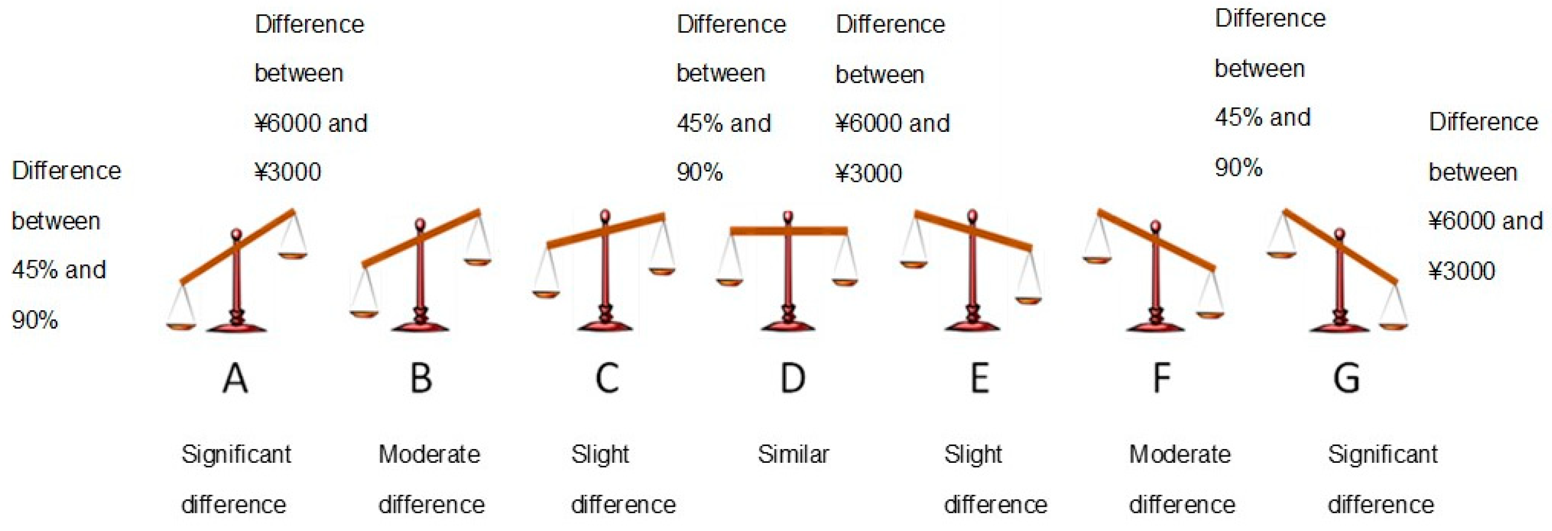
Again, we can use the gamble parameter presented in Table 1 as an example. The ETD theory posits that the difference between two options in the probability dimension (∆ Probability _{Op, Po}; 45% vs. 90%) of Game I without r multiplied was designed by Kahneman and Tversky [1] to be relatively larger than those in the outcome dimension (∆ Outcome _{Op, Po}; ¥6000 vs. ¥3000). The objective ∆ Outcome _{Op, Po} can then be subjectively equated by a decision maker, thus leading P_o to be chosen over O_p, as the former weakly dominates the latter (e.g., P_o seems as good as O_p having treated ∆ Outcome _{Op, Po} as equal, whereas P_o is definitely better than O_p in the “probability” dimension). Therefore, the ETD method of prompting people to select P_o is to make O_p as good as P_o in the outcome dimension. Then, to achieve so-called equated dominance [31] (p. 131), that is, P_o dominates O_p, the smaller ∆ Outcome _{Op, Po} that O_p is better than P_o is treated as subjectively equal.

Similarly, the ETD theory argues that the difference between two options in the probability dimension (∆ Probability _{Op, Po}; 0.1% vs. 0.2%) of Game II with r multiplied is relatively smaller than that in the outcome dimension (∆ Outcome _{Op, Po}; ¥6000 vs. ¥3000). The objective ∆ Probability _{Op, Po} can then be subjectively equated by a decision maker, thus leading O_p to be chosen over P_o, as the former weakly dominates the latter (e.g., O_p seems as good as P_o having treated ∆ Probability _{Op, Po} as approximately zero, whereas O_p is definitely better than P_o in the “outcome” dimension). Therefore, the ETD of prompting people to select O_p is to make P_o as good as O_p in the probability dimension. Then, to achieve so-called equated dominance, that is, O_p dominates P_o, the smaller ∆ Probability _{Op, Po} that P_o is better than O_p is treated as subjectively zero. Notably, making a comparison between differences in the outcome dimension (∆ Outcome _{Op, Po}) and differences in the probability dimension (∆ Probability _{Op, Po}) is meaningless and considered to be impossible in the physical world. This is because the “amount of payment” and “probability of payment” dimensions cannot be expressed in terms of the same unit of quantity (i.e., incommensurable). However, such an impossibility has to be accomplished for non-compensatory and dimensional models, such as the lexicographic semiorder (LS) rule or ETD theory, no matter how meaningless it is in the physical sense.

1.3. Some Models Similar to the Equate-to-Differentiate Model

For the observed common ratio effect (subproportionality), a few models might be able to provide alternative explanations. Some similar but different rules are the similarity-induced model [32,33,34,35], additive difference model [36], LS rule [36], and search for dominance structure rule [37,38,39]. Through comparing “ETD” with these rules, it can be made clearer what it is and what it is not.

1.3.1. Similarity-Induced Model

Rubinstein [34] and Leland [32] offer explanations of the common ratio effect based on similarity judgments. Rubinstein [34] suggests that similarities in both the outcome and probability dimensions result in a “unique” preference, and that an individual “uses a procedure that aims at simplifying the choice by applying similarity relations” [35]. In Game I, most people may consider the outcomes ($3000 and $6000) to be similar; however, this is not the case for the probability. Thus, the probability dimension is the decisive factor. Yet, in Game II, most people may consider the probabilities (0.1% and 0.2%) to be similar; however, this is not the case for the outcome. Thus, the outcome dimension is the decisive factor.

The ETD model shares some similar but different elements with the similarity-induced model. The difference between the two is that the procedure suggested by the similarity-induced model is to separately determine similarity relations. According to Hsee’s [40,41] separate–joint distinction, the similarity-induced model, therefore, is a “separate or single evaluation”. However, the procedure suggested by the ETD model is to gain knowledge of ∆ Outcome and ∆ Probability in a “joint evaluation” (e.g., the visual analog scale used in the present study is a relative intensity scale and the closeness of a location can prompt participants to jointly compare ∆ Outcome and ∆ Probability), rather than in a “separate or single evaluation”. Further, compared to the ETD model, the similarity-induced model emphasizes “similarity”, whereas the ETD account emphasizes “difference”. Emphasizing the opposite response may result in different decision outcomes. For example, in a study of “accept versus reject response mode”, Shafir [42] found that the enriched option tends to be chosen and rejected relatively more often than the impoverished option, leading to an opposite preference order.

1.3.2. Additive Difference Model

The additive difference model assumes that alternatives are first processed “vertically” by making intra-dimensional evaluations, and the results of these vertical comparisons are then summed across all dimensions to determine one’s choice [36].

The fundamental difference between the additive difference model [36] and ETD model is how information is processed. This difference can be shown in two aspects. First, although both assume an “attribute-based” rather than an “option-based” information search process (i.e., all options are evaluated along one dimension before considering the next dimension), the additive difference model is a compensatory model, while the ETD model is a non-compensatory one (i.e., not allowing high values in one dimension to compensate for deficiencies in another). Second, in the additive difference model, the determinant of the final choice is between two quantities of the same units (e.g., the greater overall prospect value), whereas in the ETD model, the determinant of the final choice is between two quantities of the different units (e.g., the greater outcome or the greater probability).

1.3.3. Lexicographic Semiorder (LS) Rule

The LS rule assumes that a decision is reached by selecting the alternative that performs best on the most important dimension and ignores all other dimensions [36]. The ETD rule is most similar to the LS rule. That is, both assume an “attribute-based” decision process and a non-compensatory decision process, and both propose a trade-off between two incommensurable quantities that have different dimensions (e.g., ∆ Outcome vs. ∆ Probability). Further, both have to face a tough-to-beat difficulty in mathematically modeling their rules, as it is an “impossible mission” to translate the inequality relation between the values of the ∆ Outcome and ∆ Probability, which have different units of quantity, into an equation.

The difference between the two is that the LS rule assumes a minimum preference threshold (ε). Individuals may vary in their preference threshold, as well as in the relative importance they attribute to dimensions. When the relative difference is larger than the preference threshold, then one’s choice would be based on this dimension; otherwise, it is based on another dimension. Specifically, if the difference between the alternatives in Dimension I is (strictly) greater than ε, then the alternative that has the higher value in Dimension I is chosen. If the difference between the alternatives in Dimension I is less than or equal to ε, then the alternative that has the higher value in Dimension II is chosen. This characteristic is similar to the aspiration level proposed by the priority heuristic [43]. For instance, the procedure of priority heuristic is setting an aspiration level (i.e., defining the aspiration level as 1/10), searching through alternatives sequentially, and stopping the search as soon as an alternative is found that satisfies the level [43]. In this sense, the priority heuristic and LS rules both assume a “separate or single evaluation”. However, the ETD model assumes a “joint evaluation” and, most importantly, never assumes such a preference threshold. It has been shown that knowledge of the importance of all attributes/dimensions (e.g., cost or casualties in the Traffic Problem reported by Tversky [44] does not permit a satisfactory explanation or prediction of observed choice preferences; however, knowledge of paired “most different” outcomes (i.e., joint evaluation of ∆ Cost and ∆ Casualties) chosen by individuals does [26] (p. 153).

Additionally, both the LS rule and priority heuristic appear to work well when the offered risky options (Options A and B) are of “single-non-zero outcomes” (for simple prospects of the form [x_A, p_A; y_B, q_B], see Kahneman and Tversky [1]), and both models seem unable to explain or predict when risky options (Options A and B) are of “multiple-non-zero outcomes” [x_A p_A, y_A q_A; x_B p_B, y_B q_B]. A similar case is that the trade-off model [45] works well for an intertemporal choice with single-dated outcome (x_S, t_S; x_L, t_L) but not for an intertemporal choice with “multiple-dated outcomes” [46]. However, when generating a worst-possible-outcome dimension and best-possible-outcome dimension to present a risky choice with “multiple-non-zero outcomes” (such as the Asian disease problem, Tversky and Kahneman [47]), the violation of the invariance axiom can be satisfactorily accounted for by a trade-off between ∆Worst Possible Outcome and ∆ Best Possible Outcome, as described by the ETD rule [31] (p. 134).

1.3.4. Search for Dominance Structure Rule

ETD theory assumes that people tend to compare the difference between two options in the outcome dimension (∆ Outcome _{Op, Po}) and the difference in the probability dimension (∆ Probability _{Op, Po}). Additionally, if ∆ Outcome _{Op, Po} > ∆ Probability _{Op, Po} (∆ Outcome _{Op, Po} < ∆ Probability _{Op, Po}), then people will treat the smaller ∆ Probability _{Op, Po} (∆ Probability _{Op, Po}) as if no difference exists (i.e., will equate them). Thus, the two options are treated as if they have a weak–dominance relationship. (Weak dominance states that if Option A is at least as good as Option B in all dimensions and Option A is definitely better than Option B in at least one dimension, then Option A will dominate Option B [48,49].

The weak–dominance relationship hypothesis of the ETD rule is similar to the search for the dominance structure rule [39]. This decision rule proposes that decision makers pass through several phases to redefine goals and options until one alternative becomes dominant over others.

Despite the fact that the search for the dominance structure rule and ETD rule are by themselves not pure dominance rules and seek to make a dominance rule applicable, their views are divergent on some important aspects. Li [25] assessed their similarity and distinction in the following three aspects.

First, the representing system in which either dominated or nondominated alternatives are subjectively represented is not exactly the same for the two rules. Thus, the use of the same heuristic procedure can lead to opposite predictions. Taking the most controversial decision area (decision making under risk or uncertainty, for example), the representing system used by Montgomery will describe alternatives in two simple, risky dimensions [37]. In this case, even if some apparent compensatory rules, such as EV, EU, and SEU, are not included in his model of searching for a dominance structure, what is inferred from the think-aloud data as the compensatory rule being used by subjects might, in fact, be the non-compensatory one because what is seen as the two simple, risky dimensions (the probability of winning and the payoff) will be considered as only one dimension (possible-outcome dimension) from the ETD theory’s point of view [21,28,30,31,50]. Second, what is an operationally good dominance structure? For the ETD rule, the answer is clear and unique: A good dominance structure is a cognitive structure where all the dominated, alternative-favouring dimensional differences have been equated. However, the search for dominance structure rule does not seem to provide a unique answer on what a good dominance structure is. A dominance structure is assumed to be a representation where one alternative has at least one advantage over other alternatives and where all disadvantages associated with that alternative are neutralised or counterbalanced in one way or another. Consequently, various decision rules can be seen as operations in the process of changing the representation. A plausible candidate for the dominance structuring operations can be a non-compensatory rule, a compensatory rule, or a combined usage of the two. In some cases, the dominance structuring operations are even similar to ‘memorial or processing failures’ [51]. Third, the search for dominance structure rule suggests that several problems associated with either non-compensatory or compensatory rules could be avoided if the rules are seen as operators in a search for a dominance structure. On the contrary, ETD rule neither intends to evade such problems nor renders different phases of the decision process where these two types of rules could be applied jointly. Finally, and most importantly, although many decision rules (five non-compensatory and three compensatory rules) are assumed to serve various local functions in each particular stage, Montgomery does not assume a rule like ETD rule that could be coherently used in search operations. Therefore, if careful tests are designed, any of these eight rules would predict other choices compared to what the ETD rule would do.

Thus, subproportionality can seemingly be achieved through two completely opposite mechanisms. Given that either PT or ETD theory can provide a testable and falsifiable explanation of what makes subproportionality work, this finding allowed us to compare the two competing theories of risky choice as by-products in the present study and to further our understanding of the mechanisms behind the present results.

The goal of the present study was twofold: prediction and explanation. Specifically, it aimed to answer the following two questions: (1) Is subproportionality a replicable and robust property, and (2) is subproportionality achieved by obeying the rules of PT or ETD theory?

2. Study 1

2.1. Participants

We intended to precisely replicate the original results in the choice problems (Problems 7 and 8, p. 267) reported by Kahneman and Tversky [1] by using similar participants and the same parameters. The replication sample size needed to be 2 ½ times the sample size of the original study, in order to lead to a reasonable level of statistical power, typically proposed to be around 80% [52]. Given the reported original sample size of 66 participants, the sample size required in Study 1 was at least 165 participants. A total of 232 college students were recruited, and 10 participants were excluded due to providing the same response to all the four evaluation tasks. Thus, the final valid data set included 222 participants (N_male = 97), and the average age was 21.13 ± 1.88 years old.

Participants were recruited online via Sojump (https://www.wjx.cn/, accessed on 11 March 2021), an online platform similar to Mechanical Turk or Qualtrics, utilized to launch nationwide e-surveys in China and extensively used in behavioral and psychological studies. Participants were guaranteed anonymity and assured there were no “right” or “wrong” answers. Their preferences and reaction times were recorded. Participants were paid ¥6 (approximately equal to 0.93 USD) Four attention-check items were included to ensure the quality of the provided data. Any participants who failed the attention check were automatically excluded and not recorded by Sojump. Data are available on the Open Science Framework (OSF) at https://osf.io/9vcaj/?view_only=365e4c56b18c4590a2a6eea00681ac53 (accessed on 11 March 2021).

2.2. Procedures and Materials

Participants were instructed to complete three tasks: choice task, prospect evaluation task, and intra-dimensional evaluation task. The choice task was presented first, followed by the prospect evaluation task and the intra-dimensional evaluation task. The order of the last two tasks was counterbalanced across participants. All three tasks were presented online using the Sojump platform. Furthermore, the study was approved by the institutional review board of the Institute of Psychology, Chinese Academy of Sciences.

2.2.1. Choice Task

To precisely replicate the modal choice that generated subproportionality, the same parameters used in Kahneman and Tversky [1] (also see Table 1) were used. The order of the two pairs of choice problems was counterbalanced. Participants were asked to choose between Option A (C) and Option B (D).

2.2.2. Prospect Evaluation Task

PT’s explanation of why subproportionality can lead people to choose differently can be better understood through viewing the mediator role that “prospect evaluation” plays in Figure 1. M (prospect evaluation results) will positively mediate the relationship between X (with or without probability multiplied by r) and Y (different choices between the larger outcome with lower probability option [O_p] and the higher probability with smaller outcome option [P_o]). Thus, path a represents the effect of X on mediator M, whereas path b represents the effect of M on Y partialling out the effect of X, path c represents the effect of X on Y.

To reach a final decision by applying the compensatory and holistic strategy (i.e., PT), knowledge of prospect evaluation results (M) can permit the prediction of choice between O_p and P_o (Y). However, we should first know which option’s prospect is relatively greater to a decision maker. The visual analog scale designed and developed by Jiang, Liu, Cai, and Li (2016) can be modified and used to gain such knowledge through a “joint evaluation” [40] (M: prospect evaluation results; see Figure 2). We predicted that the option with the greater “as-if” prospect would be chosen by a PT advocator. That is, if A–C is selected in the prospect evaluation task, which means that the overall prospect value of O_p is relatively greater than that of P_o in the decision maker’s mind, then O_p will be chosen in the choice task. Similarly, if E–G is selected in the prospect evaluation task, which means that the overall prospect value of P_o is relatively greater than that of O_p in the decision maker’s mind, then P_o will be chosen in the choice task. Thus, knowledge of prospect evaluation can allow for direct prediction of choice.

The most rigorous way to test PT using a visual analog scale is by asking participants to strictly follow the PT formula and reach the overall prospect of both Option A and Option B. However, given the constraints of limited time, knowledge, cognitive resources, and computational capacities, “the rational algorithms were mathematically complex and computationally intractable, at least for ordinary human minds” [53] (p. 2). Thus, a compromise approach favorable to PT was developed. Participants were presented with one option′s overall prospect value (calculated using the formula of ∑w(p)v(x), with γ = 0.61 and α = 2/3), whereas the other option’s overall prospect value was not given and was to be estimated, presumably, by the participants. Thus, their cognitive task was reduced to judging the other option’s overall prospect value as being either greater or smaller than the offered option.

Specifically, in the prospect evaluation task, the overall prospect value of Option A (calculated using the PT formula and given by the experimenter) was placed on the left side of the scale, while the overall prospect value of Option B (to be estimated presumably by the participant) was placed on the right side. The participants’ task was to judge the inequality relationship by indicating which option’s overall prospect value on the visual analog scale was greater. If the overall prospect value of O_p was larger than that of P_o, then the scale would tilt to the left (i.e., A–C); if the overall prospect value of P_o was larger than that of O_p, the scale would tilt to the right (i.e., E–G). Otherwise, the scale would remain steady when the overall prospect values of O_p and P_o were nearly equal (i.e., D). The steeper the scale’s slope, the larger the overall prospect value difference between the two options. Participants provided their subjective evaluation by using a 7-point scale (A–G). With the original gamble as an example, point A indicated that “45% win ¥6000 ≈ ¥130.5” (since the samples are Chinese, the calculated overall prospect value is ¥130.5 (¥ = CNY, Chinese currency unit) was significantly larger than “90% win ¥3000”; point D indicated that “45% win ¥6000 ≈ ¥130.5” was equal to “90% win ¥3000”; and point G indicated that “45% win ¥6000 ≈ ¥130.5” was significantly smaller than “90% win ¥3000”.

2.2.3. Intra-Dimensional Evaluation Task

The ETD theory’s explanation as to why subproportionality can make people choose differently can be better understood by viewing the mediator role that “intra-dimensional evaluation” plays in Figure 1. X (with or without probability multiplied by r) is significantly related to Y (different choices between the larger outcome with lower probability option [O_p] and the higher probability with smaller outcome option [P_o]) through the mediator M (intra-dimensional evaluation results). Thus, path a represents the effect of X on mediator M, whereas path b is the effect of M on Y partialling out the effect of X.

To reach a final decision by applying the non-compensatory and dimensional strategy, knowledge of intra-dimensional evaluation results (M) is insufficient to directly predict the choice between O_p and P_o (Y); thus, an additional judgment/evaluation criterion is required. That is, apart from knowing which dimension (∆ Outcome _{Op, Po} or ∆ Probability _{Op, Po}) has a relatively greater intra-dimensional difference in a decision maker’s mind as the determinant dimension, knowing which option is superior in the determinant dimension is necessary. Notably, although conceptually demanded by the LS rule [36], to determine if ∆ Outcome _{Op, Po} > or < ∆ Probability _{Op, Po} is an impossibility because ∆ Outcome _{Op, Po} and ∆ Probability _{Op, Po} are two incommensurable quantities that have different dimensions. Fortunately, the visual analog scale designed and developed by Jiang et al. [54]., which achieved another impossibility of determining which dimensional difference (∆ Payoff _{LL, SS} or ∆ Delay _{LL, SS}) is greater in intertemporal choices with single-dated outcomes, can be modified and used to determine the determinant dimension (M: intra-dimensional evaluation results) in the present risky choice, with single-non-zero outcome gambles (see Figure 3). Moreover, the knowledge of which option is superior on the determinant dimension is gained by selecting the option with a greater probability/outcome in the probability/outcome dimension.

Thereafter, we predicted that the superior option in the determinant dimension would be chosen by the ETD advocator. That is, if A–C is selected in the intra-dimensional evaluation task, which means that the intra-probability dimensional difference (∆ Probability _{Op, Po}) is relatively greater than that of the intra-outcome-dimensional difference (∆ Outcome _{Op, Po}) in the decision maker’s mind, then the P_o with greater probability will be chosen in the choice task. Similarly, if E–G is selected in the intra-dimensional evaluation task, which means that the intra-outcome-dimensional difference (∆ Outcome _{Op, Po}) is relatively greater than that of the intra-probability dimensional difference (∆ Probability _{Op, Po}) in the decision maker’s mind, then the O_p with the greater outcome will be chosen in the choice task.

The two evaluation tasks were presented in a randomized order. After completing the choice task, participants were then asked to indicate their choice by circling a letter on a scale ranging from A to G.

2.3. Results and Analysis

2.3.1. Analysis for Choice Results

To examine whether there were correlations or collinearity among different judgments across tasks, we conducted two analyses, including a correlation test and Harman’s single-factor test. The correlation test results showed no significant correlation (ps > 0.05) among the four judgment tasks (include two prospect evaluation tasks in Game I and II and the other two intra-dimensional evaluation tasks in Game I and II) except one (prospect evaluation task in Game I and intra-dimensional evaluation task in Game II) (r = 0.215, p < 0.01), indicating that the judgment tasks in our study were valid and meaningful. Additionally, to test the possible existence of common method bias in Study 1, Harman’s single-factor test [55] was performed, with all the items entered into a factor analysis. No single factor emerged, nor was there a general factor that accounted for the majority of covariance among these variables. The value of the first factor was 1.46, which could explain 24% of the variance. Therefore, common method bias is unlikely to be a serious concern in this study.

The results showed that 92% of the participants in Game I (without r multiplied) chose Option B (higher probability with smaller outcome, P_o), whereas 81% of the participants in Game II (with r multiplied) chose Option C (larger outcome with lower probability, O_p;

Table 2. Choice results from the two games in the choice task.

		Game II (with r Multiplied)		Total
		C	D
Game I (without r multiplied)	A	13	4	17 (8%)
	B	166	39	205 (92%)
	Total	179 (81%)	43 (19%)	222

Note. The underlined data are those consistent with the position of the PT and ETD theory approaches.

). This finding indicated that the modal preference asymmetrically shifts from Option B to Option C in the expected direction. The results obtained from the Chinese college student samples in the present study were essentially identical to those obtained from Kahneman and Tversky’s [1] Israeli or American participants.

McNemar’s [56] test was used to examine whether the differences between the choice proportions in the two games reached a significant level. The differences between the choice proportions in the two games were statistically significant, χ² (1) = 152.48, φ = 0.83, and p < 0.001, indicating that the majority preference, which generated subproportionality, could be successfully replicated in a sample of Chinese college students.

2.3.2. Mediation Analysis

We further examined whether the prospect or intra-dimensional evaluation results could be mediators in predicting choice shift. According to a two-condition within-participant statistical mediation analysis based on the path-analytic framework proposed by Montoya and Hayes [57], we explored if the prospect and intra-dimensional evaluation results could be the mediators in predicting the modal choice that generated the subproportionality, through mediation analysis methods. The MEMORE macro is appropriate for dichotomous outcomes and estimates the effect of the predictor on the mediator (path a), effect of the mediator on the outcome variable holding the predictor constant (path b), total effect (path c), and direct effect of the predictor (path c′).

First, we standardized all the variables before performing the mediation analysis. Then, in MEMORE, we constructed a bias-corrected bootstrap confidence interval (CI) for the indirect effect using 10,000 bootstrap samples. If zero is not between the lower and upper bounds, then the analyst can claim that the indirect effect is not zero with a 95% CI [58]. Considering that both judgments (prospect and intra-dimensional evaluations) may impact the results and given that the experiment was conducted using a within-subject design, we performed a parallel mediation analysis to include both judgment tasks.

Figure 4 presents the results of the parallel mediation analysis on prospect and intra-dimensional evaluations. As shown in the upper panel (prospect evaluations) of Figure 4, the choice shift was found (path c, p < 0.001), which means people choose differently in the two games. Then, the effect of subproportionality (with or without r multiplied) on prospect evaluation (continuous variable) results was significant (β_a = 0.57, p < 0.001). This indicated that prospect evaluation results were positively changed after r was multiplied. The beta of path b was positive but not significant (β_b = 0.03. p = 0.51), indicating that the larger number of estimated prospect evaluation results could not significantly predict the choice of a higher prospect value. Lastly, the indirect effect of manipulation “with r being multiplied” (X) on choice shift (Y) through the mediator of prospect evaluation results (M) is 0.017 and the 95% CI included zero (95% CI [−0.025, 0.072]), which means the prospect evaluation results cannot account for the choice shift as a mediator.

As shown in the bottom panel (intra-dimensional evaluations) of Figure 4, the effect of subproportionality (with or without r multiplied) on the intra-dimensional evaluation results was significant (β_a = −0.84, p < 0.001), indicating that the intra-dimensional evaluation results were negatively changed after r was multiplied. Further, path b was significant (β_b = −0.16. p = 0.003), indicating that the intra-dimensional evaluation results can predict the choice shift. Lastly, the indirect effect of manipulation “with r being multiplied” (X) on choice shift (Y) through the mediator of intra-dimensional evaluation results (M) was 0.138 and the 95% CI did not include zero (95% CI [0.050, 0.227]), which indicated the intra-dimensional evaluation results can account for the choice shift as a mediator.

To better understand the sign of the beta, we described the logic of ETD models as follows. We coded the chosen option (e.g., Option A and B) as 0 and 1, respectively. The ETD model hypothesizes that the probability dimension is superior to the outcome dimension before r is multiplied, while the outcome dimension is superior after r is multiplied. The smaller the rating on the visual analog scale, the more the probability dimension dominates the outcome dimension. Therefore, the beta of path a was negative, indicating that the difference of the probability dimension (∆ Probability _{Op, Po}) was larger than the difference of the outcome dimension (∆ Outcome _{Op, Po}). When the difference of the probability dimension is relatively greater, one’s choice will be made based on the probability dimension and will choose Option B (higher probability with smaller outcome, P_o). As a result, the beta of path b was negative.

To further examine whether the difference in the indirect effects between the two judgment tasks was significant, we performed a difference test. The results indicated that the indirect effects of both judgment tasks were significant (β = −0.117, 95% CI [−0.224, −0.014]) and the coefficients of the indirect effect in the intra-dimensional evaluation task (0.138) was larger than that in the prospect evaluation task (0.017). Our data showed that the intra-dimensional evaluation could be the mediator to account for the choice shift in parallel mediation analysis. Moreover, the same conclusion would be reached if an individual mediation analysis was performed for the prospect evaluation and the intra-dimensional evaluation independently.

In conclusion, PT and ETD theory can predict an individual’s option preference in terms of a resulting choice. However, our mediation analysis evidence indicated that the intra-dimensional evaluations suggested by ETD theory can better predict and explain subproportionality than the prospect evaluations suggested by PT.

3. Study 2

In Study 1, both PT and ETD theory would predict the same modal choice, thereby generating subproportionality. Study 2 was then designed to provide a possible critical test to discriminate between those two theories. Following Li′s logic, Li [30] suggested that the framing effect can be produced only if the framing or wording can change people′s equate-to-differentiate strategy across different frame conditions (p. 133) of investigating the framing effect [47], we reasoned that “with r multiplied” was analogous to the manipulation of framing or wording conditions. Only if the manipulation of “with r multiplied” could change the perceived relative ∆ Probability _{Op, Po,} could the so-called subproportionality be achieved. That is, participants’ risky preferences would shift in two opposite directions. Otherwise, subproportionality would not be observed, regardless of whether r was multiplied.

Accordingly, a new set of gamble parameters (see

Table 3. Experimental material in Study 2.

Game I without r multiplied A: (76,000, 42%)	B: (38,000, 84%)
Game II with r multiplied C: (76,000, 36%)	D: (38,000, 72%)

) was deliberately designed to satisfy the choice shift prediction made by PT, but not that made by ETD theory. Thus, the new set of gamble parameters would make P_o the greater prospect in Game I, while O_p would be the greater prospect in Game II, thereby leading to a prediction made by PT that subproportionality will be achieved. However, the new set of gamble parameters would leave the perceived relative ∆ Probability _{Op, Po} unchanged, leading to a prediction made by ETD theory that no subproportionality will be observed.

Additionally, several improvements were made in the Study 2. First, consistent with the causal chain perspective, the task order (first choice task, followed by prospect evaluation/intra-dimensional evaluation task) was changed to the intra-dimensional/prospect evaluation task being presented first, followed by the choice task. Second, a between-subject design was used to minimize potential mutual interference between the two scale tasks. Third, given that the choice is a binary choice task in PT (without an indifference option), the selection of the indifference option (Option D) on the 7-point visual analog scale, which is directly borrowed from the study of Jiang et al. [54], appears unable to explain or predict any choices in Study 1. Therefore, the 7-point visual analog scale with an indifference option (Option D) used in Study 1 was replaced with a 6-point scale in Study 2 to reduce statistical noise.

3.1. Participants

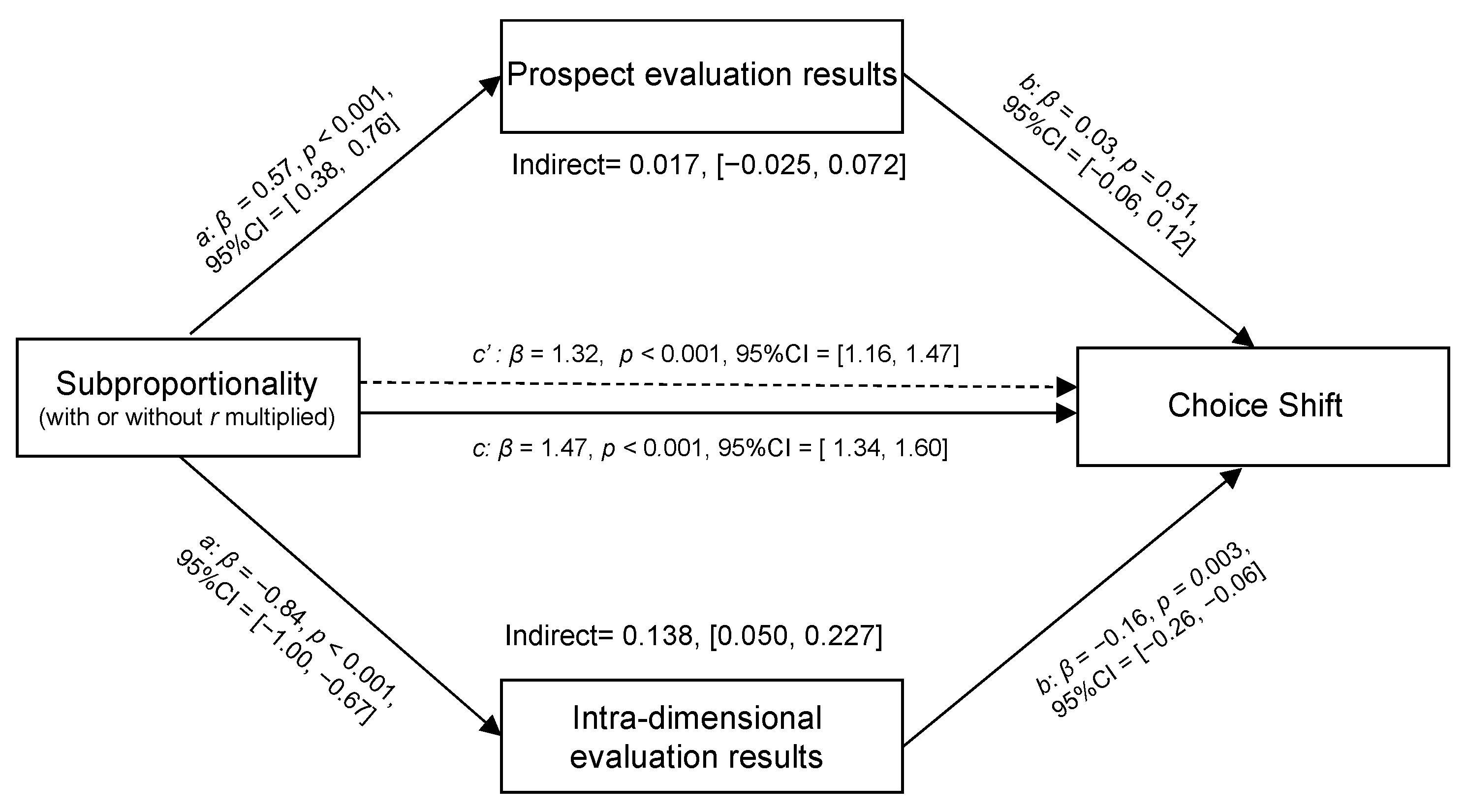
The sample size was calculated a priori to achieve at least 80% statistical power for the mediation analysis, given the coefficients of paths a and b set at 0.57 and 0.06 in the prospect evaluation task and 0.84 and 0.17 in the intra-dimensional evaluation task, based on the path coefficients calculated in Study 1 by using the method suggested by Fritz and MacKinnon [59]. The minimum sample size was 391 participants in the prospect evaluation task and 396 participants in the intra-dimensional evaluation task.

Therefore, a total of 411 college students were recruited in the PET condition (prospect evaluation task only version, PET); however,17 participants were excluded after providing the same response to all items. The final valid data set included 394 participants (N_male = 149), and the average age was 22.30 ± 3.12 years old. A total of 416 college students were recruited in the IET condition (intra-dimensional evaluation task only version, IET); however, 43 participants were excluded after providing the same response to all items. Thus, the final valid data set included 373 participants (N_male = 130), and the average age was 22.34 ± 2.60 years old.

Similar to Study 1, the sample in the Study 2 was recruited online via Sojump. Participants were paid ¥10 (approximately equal to 1.55 USD) for participating in the survey. Two attention-check items in each condition/version were used to ensure the quality of the provided data. Participants who failed the attention check were automatically excluded and not recorded by Sojump.

3.2. Procedures and Materials

Participants were asked to perform the prospect evaluation task first in the PET condition, and the intra-dimensional evaluation task first in the IET condition.

3.2.1. Prospect Evaluation Task

The participants were instructed to rate their subjective overall prospect value using a 6-point scale following the same instruction as the previous study.

3.2.2. Intra-Dimensional Evaluation Task

The participants were asked to rate their subjective intra-dimensional evaluation using a 6-point scale. The same instructions used in the previous study were used again.

3.2.3. Choice Task

The participants in both conditions (PET and IET) were then asked to choose between Option A (C) and Option B (D). The two pairs of choice problems with new gamble parameters were as follows:

Game I without r multiplied (without r = 0.86 multiplied):

• A (76,000, 42%): larger outcome with lower probability option (O_p) (CPT ≈ 682.00)
• B (38,000, 84%): higher probability with smaller outcome option (P_o) (CPT ≈ 727.59)
• Game II with r multiplied (r = 0.86):
• C (76,000, 36%): larger outcome with lower probability option (O_p) (CPT ≈ 627.45)
• D (38,000, 72%): higher probability with smaller outcome option (P_o) (CPT ≈ 618.42)

3.3. Results and Analysis

3.3.1. Analysis for Choice Results

The prediction made by PT is that a choice shift that leads to subproportionality should also be observed even if the new set of gamble parameters is applied. Contrastingly, the prediction made by ETD theory is that no choice shift that leads to subproportionality should be observed if the manipulation of “with r multiplied” could not change the perceived relative ∆ Probability _{Op, Po}.

Overall, the data showed that the majority of the participants (69%) in Game I (without r multiplied) chose Option B (higher probability with smaller outcome option, P_o). By contrast, the majority of the participants (74%) still chose Option D (higher probability with smaller outcome option, P_o) in Game II (with r multiplied (see

Table 4. Choice results from the two pairs of choices in the PET and IET conditions.

		Game II				Total
		(with r Multiplied)
		C		D
		PET	IET	PET	IET
Game I (without r multiplied)	A	63	70	58	43	234 (31%)
	B	30	39	243	221	533 (69%)
	Total	202 (26%)		565 (74%)		767

Note. The underlined data are consistent with the PT approach.

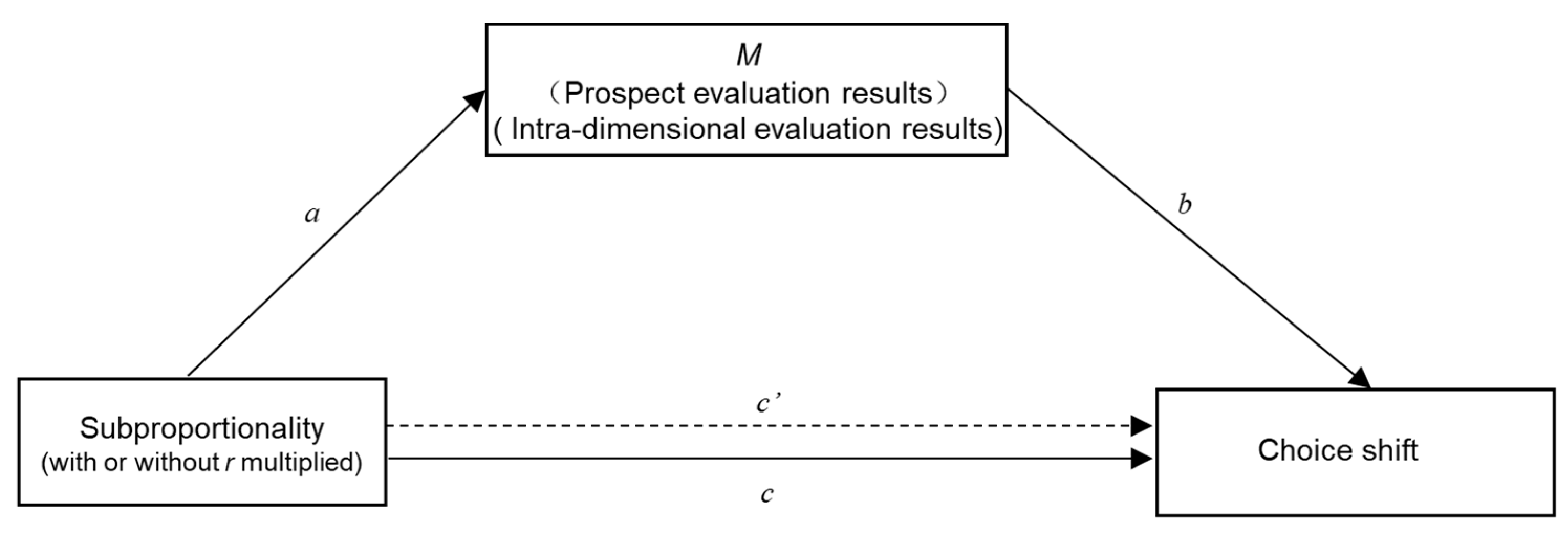
)). The difference between the choice proportions in the two games was statistically significant (χ² (1) = 5.65 (continuity corrected), p = 0.02, φ = 0.09). The findings indicated that the modal choice was inconsistent with the prediction of PT. However, whether the modal choice can be predicted by ETD theory should be analyzed by further gaining evidence from following mediation analysis that path a (see Figure 1) is insignificant.

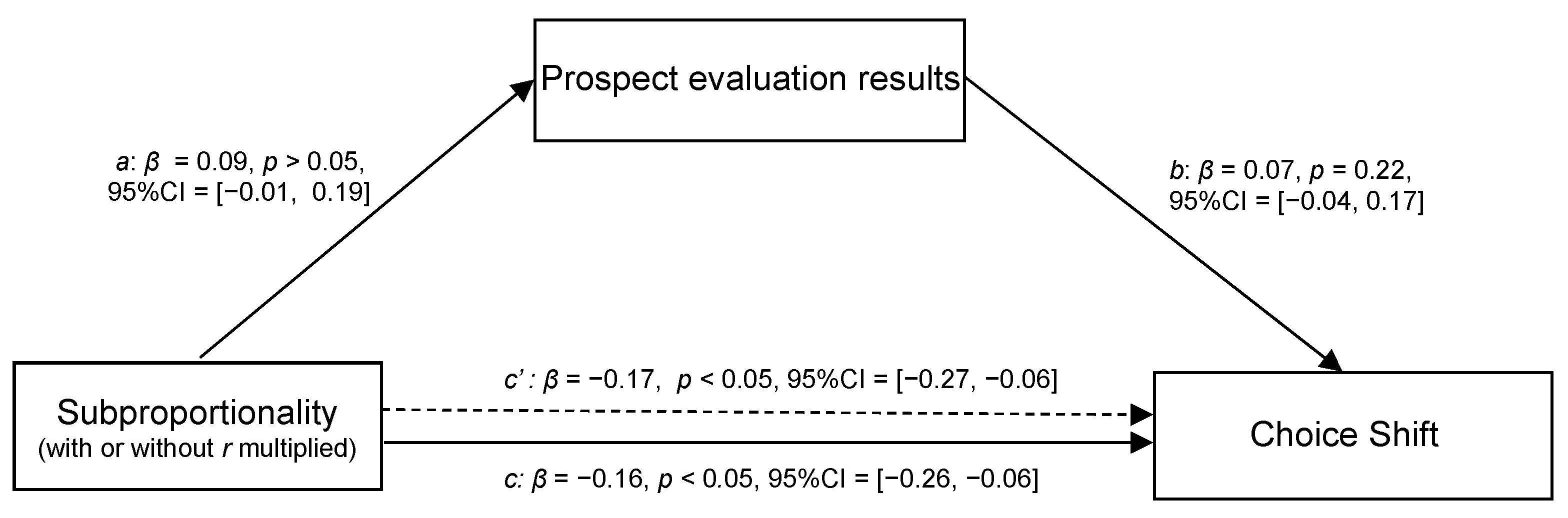
3.3.2. Mediation Analysis for the PET Condition

If one’s choice is based on maximizing the overall prospect value, as prescribed by PT, then the overall prospect value evaluation should be able to explain and predict choice shift (i.e., path b is significant). However, the data analysis showed that the prospect evaluation failed to account for choice shift (β_b = 0.07, p > 0.05) (see Figure 5).

3.3.3. Mediation Analysis for the IET Condition

If one′s choice is based on intra-dimensional evaluation, as prescribed by ETD theory, then the superior option in the determinant dimension would be chosen. That is, intra-dimensional evaluation should be able to explain and predict choice shift (i.e., path b is significant). The data analysis revealed that intra-dimensional evaluation can account for choice shift (β_b = −0.20, p < 0.001) (see Figure 6). More importantly, the finding that path a is insignificant supports our conjecture that subproportionality cannot be achieved if the manipulation of “with r multiplied” fails to change the perceived relative difference between two options in the probability dimension (∆ Probability _{Op, Po}).

As expected, the application of our modified gamble parameters generated a possible critical test to discriminate between these two theories. That is, PT and ETD theories would generate “different” outcomes. The findings demonstrated that the modal choice was inconsistent with the prediction of PT. Moreover, the choice shift cannot be accounted for by prospect evaluation but can be satisfactorily accounted for by intra-dimensional evaluation. Thus, Study 1 and Study 2 further strengthened understanding of the mechanisms underlying ETD and PT theories.

4. Discussion

In risky decision-making situations, two decision paradoxes (the Allais common consequence and Allais common ratio paradoxes) were named after Maurice Allais [60,61,62]. The Allais paradox is considered a lever that moved EU and forced those who remained steadfast in their devotion to expectations to conceive of a model engaged in a nonlinear transformation of the probability scale (for reviews, see, e.g., Machina [63]). A weighting π or a rank-dependent weighting function w was utilized by the revamped models of risky choice (e.g., prospect or cumulative prospect theory) to explain that the Allais paradox exists because people behave to maximize overall prospect value rather than the EU [9]. However, Allais has his own explanation for the Allais paradox. In his Nobel lecture, Allais states:

In fact, the “Allais Paradox is paradoxical in appearance only, and it merely corresponds to a very profound psychological reality, the preference for security in the neighborhood of certainty” [64].

The “Paradox” mentioned in this Nobel lecture is actually referred to as the “Allais common consequence paradox”. Interestingly, if Allais had posed his choice problems ([1 M, 1.00] vs. [5 M, 0.10; 1 M, 0.89; 0, 0.01]) only to Asian participants, then he might have not found the surprising and striking findings that generated the paradox. The data we collected in the classroom demonstration indicated that the most frequently chosen alternative in Allais’ first pair of choices is not the sure thing option but the risky option (for detailed demonstration, see Li, Rao, and Xu [22]). This risk-seeking behavior is somewhat more consistent with Hsee and Weber’s [17] finding that Chinese students are significantly less risk averse than Americans in their choices between risky options and sure outcomes than is suggested by Allais′ [6] finding.

Nevertheless, the modal choice, which can lead to the Allais common ratio paradox, was replicated successfully by employing Chinese student samples in the present study. Thus, PT can safely derive subproportionality if decision makers behave to maximize the overall prospect value, $\sum w\left(p\right)v\left(x\right)$. Such a finding satisfactorily answers the question: “Is it true?”.

Regarding “how can it be achieved?”, we found that, despite the fact that the overall prospect value proposed by PT is more sophisticated than that proposed by EV, EU, or SEU, among others, risk choice will unlikely be described as people behaving to maximize the overall prospect value ($\sum w\left(p\right)v\left(x\right)$), as defined by PT. The relationship between the results for the “prospect evaluation task” and “choice task” does not support the “as-if” notion that one will select the alternative with the greatest overall prospect value. Contrastingly, the relationship between the results of the “intra-dimensional evaluation task” and “choice task” is consistently in favor of the ETD theory. In arriving at such a conclusion, we considered that it is unfair to judge or evaluate one theory based on the standards of another theory. Pachur, Suter, and Hertwig [65] even suggested that algebraic/as-if models and process models should not be treated as antithetical or even incommensurable, although they rest on fundamentally different assumptions and algorithms.

Accordingly, the visual analog scale designed for the “intra-dimensional evaluation task” (an incommensurable comparison in the physical sense) aims to test ETD theory. This theory represents a process account of choices by checking whether the final decision is considered a competition between intra-outcome and intra-probability dimensional differences (∆ Outcome _{Op, Po} and ∆ Probability_{Op, Po}). The winner of the competition determines whether the final choice is simply one of choosing an option with greater “Payoff/Outcome” or an option with greater “Chance/Probability”. Contrastingly, the visual analog scale designed for the “prospect evaluation task” (a commensurable comparison) aims to test PT, which represents an “as-if” account but not a process account. The checking is based on whether the final decision is determined by selecting a greater overall prospect value, but not whether participants actually performed a lengthy process of computing and maximizing $\sum w\left(p\right)v\left(x\right)$ with v being v (x) = x ^⅔ and w being ${w\left(p\right)=p}^{\gamma }{/[p}^{\gamma }{+(1-p)}^{\gamma }{]}^{1/\gamma }$, γ = 0.61. This step is relatively reasonable because CPT analyses often do not (at least not explicitly) assume that people are able to calculate or actually calculate subjective prospect values and decision weights on the basis of the given functions [65]. Thus, we are convinced it is fair to compare two completely opposite decision mechanisms (i.e., PT and ETD theory as each mechanism′s representative) by utilizing the “prospect evaluation task” (i.e., holistically measure) and “intra-dimensional evaluation task” (i.e., dimensionally measure) developed in the present research.

Nevertheless, it could be argued that, given that the parameters (γ and α) proposed by PT vary from person to person, the chosen gamma (γ = 0.61) and alpha (α = 2/3) values tested in our study may not represent the “true” gamma and alpha values possessed by our participants. This is especially plausible, given that our participants were Chinese, whereas the participants in Kahneman and Tversky’s PT study [1] were Israeli or American, as Chinese individuals from China have been found to have more risk-seeking tendencies than Americans from the United States [17,18,19,20,66]. In such a case, the overall prospect value for a certain option (e.g., Option A of Game I in Study 1) computed by applying participants′ own values of gamma and alpha may be larger than that computed by applying γ = 0.61 and α = 2/3, which then led to Option A being ultimately selected. Thus, if our sample included those whose γ and α would lead to the overall prospect value of Option A being greater than Option B, then the number of participants who selected Option A would increase; correspondingly, the chosen proportion of Option B would be less than what PT predicted using γ = 0.61 and α = 2/3. Therefore, it would be unfavorable or unfair to test the prediction accuracy of PT by using fixed γ and α values only.

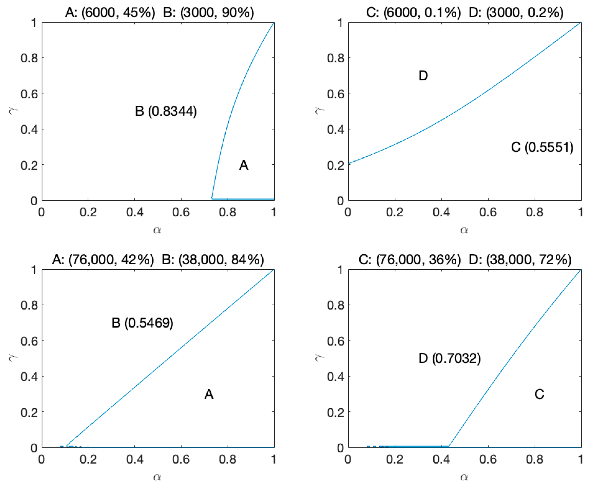
To address this concern, we assumed that each participant would have his or her own γ and α (i.e., γ and α can be any value between 0 and 1). According to the PT formula, we can calculate all combinations of γ and α and figure out the theoretical proportion for choosing the option with larger overall prospect value for the four pairs of the games ([p, x; q, y]) in our two studies (see Figure 7).

If the actual chosen proportion for choosing the riskier option (i.e., Option A) is X% by applying the selected fixed value of γ and α, we may arrive at two possible results when making a prediction by applying participants’ own “true” values of γ and α. First, PT’s theoretical prediction is larger than the actual chosen proportion (X%). Second, PT’s theoretical prediction is smaller than the actual chosen proportion (X%). Our sample should be favorable to PT if the actual proportion for choosing the option revealed by our participants is larger than the theoretical proportion for choosing the option with larger overall prospect value predicted by PT; otherwise, it is unfavorable and unfair to PT. Based on this logic, we tried to verify whether our collected sample was fair or more favorable to PT by comparing these two proportions in our studies.

By comparing the “theoretical proportion for choosing the option with larger overall prospect value” sketched in Figure 7 and the “actual proportion for choosing the option” observed in our choice task (

Table 5. The theoretical proportion for choosing the option with larger overall prospect value predicted by PT and actual proportion for choosing the option revealed by our participants in four gambles.

		Theoretical Proportion for Choosing the Option with Larger Overall Prospect Value Predicted by PT (%)	Actual Proportion for Choosing the Option Revealed by Our Participants (%)
Game I in Study 1: (A: 6000, 45%; B: 3000, 90%)	Option B	83	92
Game II in Study 1: (C: 6000, 0.1%; D: 3000, 0.2%)	Option C	56	81
Game I in Study 2: (A: 76,000, 42%; B: 38,000, 84%)	Option B	55	69
Game II in Study 2: (C: 76,000, 36%; D: 38,000, 72%)	Option D	70	74

), we can see that the theoretical proportions suggested by PT are smaller than the actual chosen proportions in the four pairs of games. This implied that our collected samples are fair to PT, or even more favorable to PT.

Results like these are neither striking nor surprising, because the LS rule proposed by Tversky [36] has a significant commonality with the ETD rule. The two rules′ predictions are based on non-compensatory and dimensional characterizations. Empirically, Tversky’s (weak) stochastic intransitivity has been demonstrated with simple lotteries. The LS strategy suggested by Tversky [36] and the simplification “editing” strategy invoked by Kahneman and Tversky [1] might explain intransitivity in simple lotteries by assuming that the choices between the first four lotteries described in his 1969 paper [36] are all based on the outcome (x) dimension. However, the choice between lotteries (a) and (e) is based on the probability (p) dimension. Thus, the probabilities of adjacent lotteries are identical, whereas the probabilities of (a) and (e) differ enough to affect evaluation and choice.

A closer look at the illustration of Tversky intransitivity may justify the inference that the mechanism underlying both the LS rule and the ETD rule is really at work from two points of view. First, Tversky [36] points out the “non-compensatory and dimensional” rules are more natural and direct, compared with the “compensatory and holistic” algorithm and may become another way to account for the mechanism underlying human decision-making behavior. The “non-compensatory and dimensional” rules mean decision makers do not need to undergo the mathematical algorithm, but can make decisions by addressing the differences between dimension directly, which is a more efficient and ecological decision-making strategy. However, the “non-compensatory and dimensional” rules present an unavoidable but difficult question when modeling: comparing incommensurable quantities. This strategy is considered to be impossible due to the requirement of comparing incommensurable quantities. For example, it is meaningless to ask whether a kilometer is larger than an hour in the field of physics.

Second, a careful reader may notice that PT (compensatory and holistic) and the LS rule (non-compensatory and dimensional) were proposed and developed by the same person. As pointed out by Li et al. [66], people might wonder why participants′ responses to the Tversky-intransitivity stimuli, which were constructed to make choices in line with a non-compensatory (non-expectation maximizing) model, are not explained by Tversky so as to be elicited by a non-compensatory process (which assumes a decision is based on only payoff (x) or chance (p) dimension), but by a compensatory one (which assumes that people choose according to an ordering implied by an aggregate of judgments of all dimensions). Notably, it can be seen that, without turning to a very natural “editing” strategy [1], which helps to explain some axiom-violating choices (e.g., cancellation editing/graph-editing operation; see also Bonini, Tentori, and Rumiati [67]; Sun, Li, Bonini, and Su [68]), it is impossible to play the game of “pitting one’s left fist (LS) against his or her right fist (PT)”. The role the “editing” strategy played in the real but not “as-if” choice is definably non-compensatory and dimensional-favored.

Decision models that approximate this line of thinking include the fuzzy-trace theory [69], heuristics, like embodied heuristics [70], and intertemporal trade-off model [45]. Fuzzy-trace theory emphasizes categorical differences and predicts that categorical differences between options are encoded as gist representations (e.g., “some money” versus “some money or no money”, “all-or-none distinctions”, and “low-versus high-danger”), while people will make decisions on the basis of the essential meaning rather than on verbatim expected values [71]. Embodied heuristics, as an early version of ecological psychology, was coined by Gigerenzer [70], that is, innate or learned rules of thumb to facilitate superior decisions. Take the baseball outfielders catching the ball as an example. It has been proven by the experimental studies that experienced players catch a fly ball by using a heuristic, not assuming players can make complex calculations unconsciously. Scholten and Read [45] further explored the domain of intertemporal choices and proposed that such choices are made by directly weighing time differences against money differences in the trade-off model. A few existing decision models have adhered to the non-compensatory and dimensional rule and assumed that people rely on only one (or a few) key dimension(s) rather than integrate information from all dimensions of an option to reach a decision [43,72].

The underlying mechanism we have shown by measuring “intra-dimensional evaluation” is that the risky choice of simple prospects of the form (x, p; y, q; simple lotteries) is dictated by a dimension-based strategy [36,73]. The knowledge on the “intra-dimensional evaluation” results would indeed permit the prediction of option preference. The observed preference can be adequately accounted for by assuming that the great outcome-dimensional difference (∆ Outcome _{Op, Po}) serves as the determinant for the larger outcome with lower probability option (O_p), whereas the great probability-dimensional difference (∆ Probability_{Op, Po}) serves as the determinant for the higher probability with smaller outcome option (P_o).

Notably, the Allais common ratio paradox is a risky choice of simple prospects of the form (x, p; y, q; simple lotteries), with a hidden zero frame. However, the Allais common consequence paradox [6] is not a simple lottery, but has an explicit zero frame. Likely, the different “zero” frames will produce different choices (c.f., Savage′s own preference pattern violated his sure-thing principle when describing Allais’ problems in a verbal format but obeyed his sure-thing principle when describing Allais’ problems in a tabular lottery format (for more detailed discussion, see Pope [74]). Given that the description of Allais′ common ratio paradox problems, which we posed to our participants, is in a hidden zero frame (x, p; y, q), we decided not to include a zero complement in our visual analog scale. Researchers interested in the hidden zero effect [75] might run an additional study to add a zero complement to the visual analog scale. The way “zero” outcomes are matched for an intra-dimensional evaluation has been well demonstrated by Li [76] (p. 421, Table 4).

Furthermore, the logic applied in the present study could provide us with new guidance on the route that future research might follow. By utilizing the “intra-dimensional evaluation” method, we can analyze and classify other properties of the probability weighting function (π function; e.g., subadditivity, overweight low-probability, and subcertainty; see also Li [13]) by identifying whether the impact posed by these properties or effects is focused on outcome-dimensional (∆ Outcome _{Op, Po}) or probability-dimensional differences (∆ Probability _{Op, Po}). Thus, we can obtain a clear understanding of which group of properties or effects can exert influence on individuals’ risky choices by shifting the perceived relative differences between the two options in the probability dimension (∆ Probability _{Op, Po}), or which group of properties or effects can exert influence on individuals′ risky choices by changing the perceived relative difference between the two options in the outcome dimension (∆ Outcome _{Op, Po}), from the perspective of decision strategy. Based on such classification and prediction, the equate-to-differentiate model (the predictions of this model are based on non-compensatory and dimensional characterizations; for the extension of its intra-dimensional strategy to a self-generated/fictional dimension, see Zheng, et al. [77] or Zhao, et al. [78]) can theoretically make a timely contribution as an effective and accurate guide for people when making optimal risky choices.

Finally, the theory of Choice Wave and Parallel Rationality is also worth mentioning. Johnson [79] questioned the classical rationality and proposed that people are indeed different, but this point had been missing from economics. Choice Wave describes consumers to make different choices at each decision point but still maximize utility every time and be rational. Just as in quantum mechanics, you do not know what the actual utility maximizing for a consumer will be until that consumer actually makes the choice.

Choice wave emphasis the importance of individual difference. This implies that data sets containing multiple types of individuals should be split according to the types [80] We think it could be helpful to split the participants into subgroups according to their choice wave type in the future, to further accurately reflect individuals′ strategy.