Article

A Strong-Form Off-Lattice Boltzmann Method for Irregular Point Clouds

Chair of Brewing and Beverage Technology, TUM School of Life Sciences, Technical University of Munich, 85354 Freising, Germany
*
Author to whom correspondence should be addressed.
Symmetry 2021, 13(10), 1802; https://doi.org/10.3390/sym13101802
Submission received: 28 July 2021 / Revised: 14 September 2021 / Accepted: 15 September 2021 / Published: 28 September 2021

Abstract

:
Radial basis function generated finite differences (RBF-FD) represent the latest discretization approach for solving partial differential equations. Their benefits include high geometric flexibility, simple implementation, and opportunity for large-scale parallel computing. Compared to other meshfree methods, typically based upon moving least squares (MLS), the RBF-FD method is able to recover a high order of algebraic accuracy while remaining better conditioned. These features make RBF-FD a promising candidate for kinetic-based fluid simulations such as lattice Boltzmann methods (LB). Pursuant to this approach, we propose a characteristic-based off-lattice Boltzmann method (OLBM) using the strong form of the discrete Boltzmann equation and radial basis function generated finite differences (RBF-FD) for the approximation of spatial derivatives. Decoupling the discretizations of momentum and space enables the use of irregular point cloud, local refinement, and various symmetric velocity sets with higher order isotropy. The accuracy and computational efficiency of the proposed method are studied using the test cases of Taylor–Green vortex flow, lid-driven cavity, and periodic flow over a square array of cylinders. For scattered grids, we find the polyharmonic spline + poly RBF-FD method provides better accuracy compared to MLS. For Cartesian node layouts, the results are the opposite, with MLS offering better accuracy. Altogether, our results suggest that the RBF-FD paradigm can be applied successfully also for kinetic-based fluid simulation with lattice Boltzmann methods.

1. Introduction

In the last three decades the lattice Boltzmann method (LBM) has grown into a successful tool for computational fluid dynamics including single- and multi-phase flows [1,2], flows in porous media [3,4], heat and mass transfer [5,6,7], and other complex flows [8,9]. The main properties underlying this success include the algorithmic simplicity of the method with its particle-like nature, a high parallel efficiency due to the large degree of local operations, and the simple handling of boundary conditions via bounce-back type methods [10,11], among others. These properties are a result of the ingenious coupling between the velocity and spatial discretizations in such a way that the spatial grid corresponds to the characteristics of the discrete velocity space [12]. On the computational level this gives the stream-collide algorithm, where collision is a set of local arithmetic operations, and the streaming of particles occurs via a simple shift of values in the memory [13].
Simultaneously, the coupling between momentum space and physical space restricts the method to uniform Cartesian grids, which are often disadvantageous for the study of flow in complex geometries [12]. Moreover, the standard lattice symmetric stencils in 2-d and 3-d, that is, those including only the neighbors from the first Brillouin zone, such as D2Q9 and D3Q19, do not guarantee sufficient degrees of freedom and lead to the loss of Galilean invariance at finite Mach numbers. This limits LBM’s domain of applicability to weakly-compressible athermal flows [14,15]. Specifically, it is the lack of a cubic term in velocity due to the second order truncation of equilibrium, which leads to an error in the viscous momentum flux at Navier-Stokes level. Due to the aliasing of velocity moments, this error can only be corrected partially [14]. While several existing integer-based multi-speed lattices can overcome this issue and simultaneously extend LBM’s applicability into the compressible flow regime, these lattices usually contain more velocities than needed based upon symmetry requirements. Due to insufficient isotropy, these extra lattice degrees of freedom are then tied-up in tensorial isotropy constraints, leaving little room for stability [16]. Moreover, the large stencil sizes lead to a decrease in computational efficiency and complications in the prescription of boundary conditions [17].
Aside from the cubic error term, the low isotropy of the standard lattices is also a source of anisotropic non-linear truncation errors [18]. The spatio-temporal coupling also limits the method to second order accuracy in time and space. Recently, the spatial and temporal errors have been identified as the culprit for numerical instability via a mechanism involving the collision of eigenvalues [19]. These findings justify the previous and more recent inquiries into stabilization strategies that can be divided into three mutually non-exclusive approaches: advanced collision operators [15,20,21,22], multiscale refinement methods [23,24,25,26], and finally—alternative time-stepping/streaming methods [12,27,28,29].
The most straightforward approaches are advanced collision operators. For a comprehensive comparison and discussion of the many available collision operators we refer the reader to the recent works [30,31]. Although these advanced collision operators are able to drastically improve the stability of the LBM in the low viscosity limit, they do not fundamentally change the behavior at the macroscopic level per se. This is in fact determined only by the choice of discrete velocity set and shape of the equilibrium distribution function [18,32] (historically, differences were observed because the equilibrium distributions were truncated at second-order).
The second approach to removing the destabilizing errors from insufficiently resolved wavelengths is temporal and spatial refinement. For the classic streaming LBM, the strong lattice coupling limits this approach to block-structured grids (i.e., quadtrees in 2-d, octrees in 3-d), where the ratios between cells and time-step sizes on different grid levels are integer values. The challenge in this approach is the correct transfer of values between different grid and time levels leading to several different reconstruction techniques. Unless designed carefully, these operations risk creating new instabilities and present formidable challenges in terms of coding and parallel performance [33]. Due to the exponential growth in computation dictated by the second order spatial and time step scaling, the multiscale refinement can be considered a necessity for performing engineering computations of practical interest. A fixed upper limit exists for this strategy in terms of the available hardware resources and computation time.
Both strategies outlined above are primarily aimed at preserving the exactness of the streaming step; contrarily, the third approach does away with it. Instead, streaming is performed via Eulerian or semi-Lagrangian methods, giving rise to the family of off-lattice Boltzmann methods (OLBM). The immediate reward is a large gain in geometric flexibility, allowing the usage of smoothly varying non-uniform grids or point clouds, and the possibility of adopting several advantageous symmetric velocity sets with higher order isotropy [34]. These lattices are able to capture non-equilibrium effects in the rarefied and compressible regimes with fewer velocities than their integer-based counter-parts [35]. In multi-component flows, the off-lattice approach allows particles with different molecular weights to propagate at different speeds [36,37] in a kinetically consistent manner. The price to pay is an increase in computational cost, since the exact memory shift of the streaming step is now replaced by a series of floating point operations. Unless designed carefully, the off-lattice streaming step can also increase the dissipation and dispersion errors of the numerical scheme [38]. To a certain extent, the losses in computational efficiency and accuracy can be countered by the increased order of spatial accuracy [39], which becomes possible once the lattice-based streaming is left behind. A recent effort to also increase the temporal accuracy can be found in [40]. In addition, the possibility of using irregularly distributed points adapted to the specific geometry can help reduce the amount of computation for a given level of accuracy [41].
Previous efforts in this direction have mostly relied on classical PDE discretization techniques [42,43,44]. Due to the stiffness of the collision operator, most early OLBMs suffered from a stringent time-step condition, limiting them to low Reynolds number (isothermal) flows. This limitation was later overcome in [12] by combining the classic variable transformation technique from [43,45] with a discretization of the advective term along characteristics [28]. The collision term is then integrated implicitly at explicit cost. An alternative explanation for this special feature of LBM was later provided in terms of Strang splitting [46]. Since the splitting procedure brings significant gains in time-stepping efficiency, most of the (Eulerian) off-Lattice Boltzmann methods developed in the past decade have aimed to preserve this feature.
Among kinetic-based simulation methods, the Taylor least-squares interpolation supplemented LBM (TLS-LBM) by Shu et al. [47] is the first example of a meshfree LBM. It relies upon a semi-Lagrangian streaming step in combination with least-squares for the spatial approximation. While applied successfully for the simulation to several flow benchmarks, the method was only demonstrated using structured grids. As indicated by Bayona (2019) [48], the least squares approach remains viable only for low-order approximations, limiting further improvements of the TLS-LBM. More recently, several weak-form meshfree LBM methods have been developed by Musavi et al. [49,50] and Tanwar (2018) [51]. Similar to grid-based weak-form discretizations methods like FEM, these meshfree LBMs require an additional quadrature step (typically involving an additional background grid), increasing the complexity of the method and resulting in an implicit system of equations. Given the shortcoming of the weak-form meshfree LBMs, it is natural to wonder whether or not their strong-form cousins are more suitable candidates for computational kinetic simulations with discrete velocity models such as LBM.
In this paper, we demonstrate this notion by developing a strong-form OLBM (SF-OLBM) for irregular point clouds. The basic version of our SF-OLBM combines an RBF-FD discretization in space with the Lax–Wendroff method in time, resulting in an intuitive and finite-difference-like numerical scheme. While considerably simpler than the weak-form meshfree LBM methods, the SF-OLBM is able to achieve comparable accuracy and computational efficiency. We demonstrate and compare these methods using a small set of numerical benchmarks including the Taylor–Green vortex flow, the lid-driven cavity, and the periodic flow in a square array of cylinders.
The rest of the paper is structured as follows. The SF-OLBM will be explained in Section 2, with details of the governing lattice Boltzmann equations, the spatial and temporal discretization methods, and the boundary conditions. A brief explanation of the point generation process concludes the section. In Section 3, the verification and validation of the proposed method is performed using the above-mentioned benchmark flow cases. This includes the evaluation of the spatial convergence rates, a demonstration of the ability to use geometry-adapted point clouds, and the effect of boundary conditions.

2. Method

This section presents the governing equations, the numerical formulation of the SF-OLBM, the boundary conditions, and the point cloud generation procedure.

2.1. Governing Equations

Our starting point is the discrete velocity Boltzmann equation (DVBE),
f i t + c i · f i = C i ( f ) ,
for the single-particle distribution function f i ( x , t ) (PDF) which is a continuous function of space and time. The subscript i refers to the set of microscopic velocities c i , where i = 1 , , q . In the classical kinetic theory of gases, the particle velocity is a continuous variable, but in the DVBE it is limited to a finite set of velocities [46], also known as the lattice. The left-hand side of (1) describes the flight of particles along straight lines dictated by the velocities c i , while the right-hand side is the collision operator C i ( f ) that couples the dynamics of the individual equations through its dependence on all of the PDFs, f = ( f 1 , , f q ) T . Without loss of generality we limit ourselves to the famous D2Q9 lattice, where the c i are given as:
c i = ( 0 , 0 ) θ i = ( i 1 ) π / 4 , i = 0 ( cos θ i , sin θ i ) , θ i = ( i 1 ) π / 4 , i = 1 , 3 , 5 , 7 2 ( cos θ i , sin θ i ) , θ i = ( i 1 ) π / 4 , i = 2 , 4 , 6 , 8 .
The low isotropy of this lattice makes it suitable only for incompressible and weakly-compressible flows. Since the focus of this paper is on spatio-temporal discretization, we limit ourselves to the lattice BGK collision operator:
C i BGK ( f ) = 1 τ f i f i ( 0 ) ( δ ρ , u ) ,
with a single relaxation time τ . The equilibrium distribution function is given by:
f i ( 0 ) = t i δ ρ + ρ 0 c i · u c s 2 + ( c i · u ) 2 2 c s 4 u · u 2 c s 2 ,
where the value, δ ρ = ρ ρ 0 , is the density fluctuation around a mean density ρ 0 . The values t i are the set of lattice weights and c s = 1 / 3 is the lattice speed of sound. The equilibrium above is in the incompressible form [52], meaning for steady flows it leads to results in agreement with the incompressible Navier–Stokes equation. The density fluctuation and macroscopic velocity are calculated from the particle distribution functions as the zeroth and first order moments with respect to the particle velocity,
δ ρ = i = 1 q f i , u = 1 ρ 0 i = 1 q c i f i .
The pressure can be calculated from the state equation p = ρ c s 2 . The viscosity of the fluid is ν = τ c s 2 .

2.2. Numerical Solution Procedure

The success of (standard) LBM can be, in part, attributed to the unique spatio-temporal discretization based upon Strang splitting [46]. This way, the collision dynamics are integrated implicitly, at the cost of an explicit method. Solution of (1) is performed in two steps, collision:
f ˜ i ( x , t ) = f i ( x , t ) Δ t τ + Δ t / 2 f i ( x , t ) f i ( 0 ) ( x , t ) ,
and streaming:
f ˜ i t + c i · f ˜ i = 0 .
To achieve good bandwidth and limit computation costs it is crucial to design the discretization of (7) in a way that satisfies the hyperbolic character of advection. A survey of other OLBMs including FDM, FVM, and others, shows that almost all methods rely upon some form of hyper-viscosity, most typically through upwinding. In this work, we apply the standard Lax–Wendroff method for temporal discretization of the advection equation.

2.2.1. Temporal Discretization

We use the Lax–Wendroff scheme for temporal discretization. First, the particle distribution function is expanded in a Taylor series with respect to time:
f ˜ i n + 1 = f ˜ i n + Δ t f ˜ i t n + Δ t 2 2 2 f ˜ i t 2 n + O ( Δ t 3 ) .
The superscript n refers to a discrete time instance, that is, t n = n Δ t . By using the advection Equation (7) we can replace the temporal derivatives with derivatives in space,
f ˜ i t n = c i α f ˜ i n x α , 2 f ˜ i t 2 n = c i α c i β 2 f ˜ i n x α x β .
Substituting these into the Taylor series (8) and neglecting the third-order terms we arrive at the following time-stepping relation:
f ˜ i n + 1 = f ˜ i n Δ t c i α f ˜ i n x α + Δ t 2 2 c i α c i β 2 f ˜ i n x α x β .
The same time discretization has been used previously in the general characteristic-based OLBM [12], as well as the weak-form meshless OLBM variants [49,53].

2.2.2. Spatial Discretization

We perform the spatial discretization using a meshfree local strong-form method [54], which can be seen as a generalization of several meshfree methods including the moving least squares approximation method (MLS), radial basis function-generated finite difference method (RBF-FD), generalized finite difference method (GFDM), diffuse approximate method (DAM), local radial basis function collocation method (LRBFCM), collocated discrete least squares method (CLSM) and many others.
The basic principle of these methods is to approximate the differentials operator as a weighted sum of function values over a local support domain, { x k } k = 1 n . For a linear differential operator L acting on a field u ( x ) the approximation is written as:
( L u ) ( x c ) k = 1 n w k u k ,
where u k = u ( x k ) and x c = x 1 is known as the center of the approximation. For the Lax–Wendroff method in 2-d, the operators required are the advection operator,
c i α x α = c i x x + c i y y ,
and the second order operator,
c i α c i β 2 x α x β = c i x 2 2 x 2 + 2 c i x c i y 2 x y + c i y 2 2 y 2 .
The sub-methods listed above differ in the way the weights w k are generated, using different underlying trial functions for the construction of the approximation. The detailed procedures for generating the weights can be found in the literature. Herein, we only studied the MLS [54] and RBF-FD [55] approximations. Computational routines for both types of approximation are available in specialized libraries [56]. Compared to weak-form OLBM methods, the strong-form methods obviate the need for an integration step, rendering an explicit system of equations (the mass matrix is equal to the identity matrix).
The weights for each stencil are calculated by solving a small system of linear equations at each node. For a chosen approximation method, assembly of the linear system only requires knowledge of the stencil coordinates. The weight computation is only performed once before the simulation begins (as long as the nodes are static). For the computer implementation, we assemble the weights into set of sparse matrices for each velocity direction c i . The sparsity pattern of the matrices equals the graph of nodal connectivity. After assembly and selection of the time step size Δ t , the time-update (9) is performed by repeated sparse matrix-vector product (SpMV) operations.

2.3. Boundary Conditions

For flows around objects or in bounded domains, correctly capturing the boundary conditions is a crucial part of the calculation. Typically, the boundary conditions are prescribed only in terms of the macroscopic variables and act as a constraint upon the underlying particle distribution functions. Since the strong-form OLBM assumes that the distribution functions reside at the nodes we adapt a regularized procedure [57], where the boundary populations are reconstructed according to:
f i ( x w , t + Δ t ) = f i ( 0 ) ( ρ w , u w ) + f i ( 1 ) ( ρ w , S ) ,
where x w is a wall node and u w is the prescribed wall velocity. The equilibrium part depends only on the macroscopic boundary conditions. The density ρ w can be computed using lattice symmetries, or extrapolated from the previous time step. The non-equilibrium correction f i ( 1 ) [11] is computed from the strain-rate tensor S using:
f i ( 1 ) ( ρ , S ) 2 w i τ ρ c s 2 Q i : S ,
where Q i = Q i α β = c i α c i β c s 2 δ α β and the symbol: means tensor contraction. The strain-rate tensor is evaluated either from the velocity field u ( x , t ) using the definition S = 1 2 u + ( u ) T . Here, the discrete differentiation operators (10) can be used. Alternatively, the strain-rate tensor can be evaluated from the non-equilibrium part of the distribution function using the regularization technique [57]. This was the strategy we adopted here.

2.4. Point Cloud Generation

One of the advantages of meshfree methods is they can avoid the difficulties associated with traditional polygonal mesh generation techniques. Instead, several heuristic sampling techniques that can generate well-conditioned points sets have been developed in recent years [58,59]. An overview of different point cloud generators can be found in the work of Slak and Kosec [60].
In this work we have used two kinds of point-cloud generators. For the periodic flow benchmarks we have relied on a periodic Poisson disk sampling algorithm with a fixed background grid for fast neighbor searching and distance calculations. At the periodic boundaries we use modulo arithmetic to find the indexes of the neighbor cells. In two dimensions, the 24 neighbor cells are searched. If there are objects in the domain, we first place equally spaced nodes on the object boundary. Any sampled points that are outside of the domain are rejected. For non-periodic flow cases we have relied on the point cloud generator described in Ref. [60]. This generator provides node sampling according to a target density function, for example, for placing nodes more densely near boundaries. For simple domains (e.g., rectangles) we can use the classic stretching functions such as the sine and inverse tangent ones. Herein, we have decided to use a signed distance function (SDF) approach adapted from the distmesh generator. The signed distance function returns the shortest distance from any given point to the boundary of the object at a given point. For geometric shapes such as squares, rectangles, circles, and ellipses, the SDFs are known analytically and can be combined using the operators from constructive solid geometry to build complex shape domains. The inside and outside regions of the domain differ in sign, while the boundary is located precisely on the zero level set curve (in 2-d). Using a given SDF we can prescribe a nodal density function according to:
δ r ( x ) = r min + ( r max r min ) 2 L sdf ( x ) ,
where r min is the minimal allowable distance between nodes (e.g., the spacing at the boundaries), and r max is the maximal allowed spacing, for a domain with characteristic dimension L.
Afterwards, the generated points are organized into a k-d tree for fast spatial searching. For two-dimensional periodic domains, the points can be mapped to the surface of a torus and the neighbor searches are then performed in three-dimensional space [55]. Since the torus mapping is only locally distance preserving, the resulting support sets are different from what we would expect if the neighbor searches were performed in 2-d. The partial differential equations should then also be mapped to the surface and solved using the three-dimensional mapped operators. Instead, we have decided to apply a 2-d tiling strategy. First, we create a tiling of the initial periodic point set that is translated in the axis-directions (in 2-d we need three tiles if a single axis is periodic and nine tiles if the domain is periodic in both). Spatial neighbor searches are performed only for the center tile. We recover the nodal indexes in the center tile by taking the remainder in the division of the tiled index with the number of nodes in the center tile. Bear in mind that when inter-nodal distances are calculated using only the node positions in the original (center) tile, a correction is needed due to the periodicity.
Finally, to improve the conditioning of the generated node sets we apply an annealing process based upon a repulsive force between nodes similar to the ones described in [60,61]. An example point cloud generated by the periodic Poisson disk sampling and the following annealing procedure are shown in Figure 1.

3. Results

For the verification and validation of the SF-OLBM we have used three flow benchmarks: the Taylor–Green vortex flow, lid-driven cavity flow, and the flow over a periodic square array of cylinders. These benchmarks were selected to demonstrate the beneficial properties of our approach including the adjustable spatial accuracy and the ability to use irregular point clouds.
Unless stated otherwise, the constant part of density was set to ρ 0 = 1 , the minimal spacing between points was h = 1 , and the time step was chosen according to δ t = h CFL / | c i | max , where C F L = 0.1 . The ratio of Δ t / τ was then free to vary, depending on the viscosity ν = τ / c s 2 . For stationary flows we used the following convergence criterion:
x | u ( x , t ) u ( x , t 1000 δ t ) | 2 x | u ( x , t 1000 δ t ) | 2 < 10 7 ,
where the sum is taken over the nodes in the simulation domain.

3.1. Taylor–Green Vortex Flow

To test the accuracy of the proposed OLBM in the absence of boundary effects, we first apply it to Taylor–Green vortex flow in two dimensions. The analytic solution for this fully periodic flow is given by:
u a ( x , t ) = u 0 k y / k x cos ( k x x ) sin ( k y y ) exp ( t / t c ) v a ( x , t ) = u 0 k x / k y sin ( k x x ) cos ( k y y ) exp ( t / t c ) ,
for velocity, and
p a ( x , t ) = p 0 ρ u 0 2 4 k x k y cos ( 2 k x x ) + k x k y cos ( 2 k y y ) exp 2 t / t c ,
for pressure. Here, u 0 is the initial velocity amplitude, k = ( k x , k y ) is the wave vector, p 0 is a reference pressure value, ν is the shear viscosity, and t c = ν ( k x 2 + k y 2 ) 1 is the vortex decay time.
Using the macroscopic values from the formulas (17) and (18), the initial values of the distribution function at t = 0 are set to their equilibrium values f i ( x , 0 ) = f i ( 0 ) ( ρ a ( x , 0 ) , u a ( x , 0 ) ) .

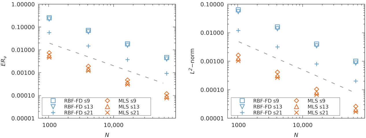
3.1.1. Spatial Errors on Scattered and Cartesian Point Clouds

We evaluate the spatial convergence on scattered (S) and Cartesian (C) point clouds for three stencil sizes (9, 13, and 21). Details of the approximations, along with their abbreviations, are provided in Table 1. For the RBF-FD stencils we use polyharmonic splines (PHS) augmented with polynomials (also known as PHS + poly). The MLS-based stencils use a polynomial basis and a Gaussian weight function. The scattered point clouds (see Figure 2b) were generated according to the procedure described in Section 2.4. Due to the irregular packing the scattered node sets contain fewer nodes than the Cartesian ones for the same domain size.
The computational domain is set to 0 < x , y < L for the domain sizes L L 0 , 2 L 0 , 4 L 0 , 8 L 0 where L 0 = 32 . We consider only the case with unity aspect ratio k x = k y = 2 π / L . The kinematic viscosity is set to ν = 0.01 and the initial velocity on the coarsest grid is chosen as u 0 = 0.01 in order to limit the effect of compressibility errors. The simulations are run until t = ln ( 0.01 ) t c , when the initial wave amplitude has decayed by two orders of magnitude. Measurements of the error norms (see Equation (19)) and maximum velocity (wave amplitude) are performed every 100 ( L / L 0 ) 2 / CFL time steps for times t > ln ( 0.1 ) t c . The delay before starting measurements is to allow any remaining inconsistency in the initial condition that could lead to oscillatory behavior of the solution to die out. Following the procedure outlined in [22] (cf. Section 5.1, p. 518), we measure the viscosity of the fluid ν m by fitting a linear function to the logarithm of amplitude values, ln ( | u | max ) . The slope of the fit corresponds to the viscosity coefficient.
Using the set viscosity ν , we determine the relative error in viscosity, ER ν = | ν m ν | / ν , as a function of the number of nodes N. The results are plotted in Figure 3 and Figure 4 for the Cartesian and scattered node sets, respectively. Additionally, we show the L 2 -norm of velocity at the final time t = ln ( 0.01 ) t c calculated as:
L u 2 = x u ( x , t ) u a ( x , t ) 2 x u a ( x , t ) 2 .
For Cartesian node layouts, in Figure 3 we observe second order convergence behavior for both the MLS and RBF-FD discretizations. Interestingly, the viscosity and velocity errors of the MLS discretization are one order of magnitude lower than the RBF-FD ones. A modified equation analysis of the discrete Lax–Wendroff operators to identify the leading error terms could shed more light on this result. For the PHS + poly RBF-FD method, larger stencil sizes lead to smaller errors in agreement with previous findings [61,62]. At a fixed polynomial degree of the RBF-FD, the polynomial terms take over the initial terms in the Taylor expansion of the approximated function, while the additional RBF terms act on the remaining error, thereby slowly decreasing the error with an increase in stencil size. For the MLS approximation, the effect of stencil size is less dramatic, although a more definitive study would also need to consider the weight function influence [48].
For scattered point clouds the spatial convergence results are shown in Figure 4. Compared to the calculations on Cartesian grids, the results are here markedly different. The residual errors of the MLS and RBF-FD approximation now display similar magnitudes. With large N the residuals of RBF-FD decrease faster than the MLS ones, giving an advantage to the PHS + poly RBF-FD when used on irregular point clouds.

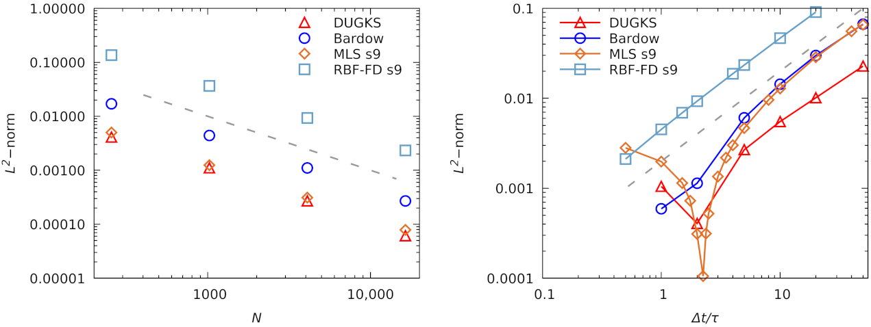
3.1.2. Comparison with Other Methods

In Figure 5, we compare the spatial and temporal accuracy of the SF-OLBM with other off-lattice approaches, including the general characteristic-based algorithm of Bardow [12] and the DUGKS method [63]. Values of the L 2 -norm (19) were extracted from [63] (see Table 1 and Figure 4 therein). The settings used in their Taylor–Green benchmark were Ma = 0.01 , Re = 100 , and k x = k y = 2 π / L . The error values were measured at the vortex half-life time t = ln ( 2 ) t c .
The spatial accuracy measurements were performed at four increasing grid sizes with a fixed time-step Δ t = 2 τ to keep the temporal errors small. For fair comparison, in Figure 5 (left) we have only included the measurements of MLS and RBF-FD with a stencil size of nine points, equal to the finite volume stencils used in the original source [63]. The MLS accuracy on the Cartesian node layout compares favorably with the DUGKS method, given that the latter is twice as expensive. As already found earlier, the RBF-FD set-up leads to poor results on regular grids.
For temporal accuracy, a grid of size 64 × 64 was used while the ratio Δ t / τ was varied at fixed τ . As can be seen from Figure 5 (right), the accuracy of MLS is close to that of the method of Bardow, while the errors of the RBF-FD stencil with nine nodes are again larger. For the highest measurement point Δ t = 50 τ the RBF-FD diverged (also for larger stencil sizes) indicating insufficient dissipation at large ratios of Δ t / τ . Interestingly, the MLS error shows non-monotone behavior with a local minimum appearing close to Δ t 2.2 τ . A cancellation of leading error terms (including those from the collision step) is a possible explanation. Similar minima might also occur for the DUGKS and Bardow methods but are missed by the coarse sampling used in [63].
As a rough performance estimate, we also give the computation times needed for 10,000 evolution steps measured on a single core of an Intel(R) Core(TM) i7-7700K CPU @ 4.20 GHz processor. All computations were performed using 64-bit double precision floating point numbers. The results for different mesh and stencil sizes are summarized in Table 2. We find the performance of the SF-OLBM to be comparable to or slightly better than other available reports [41,63]. Due to different hardware, amount of optimization effort, compiler flags, data structure memory layout and other computational issues, the timings should be approached with caution.

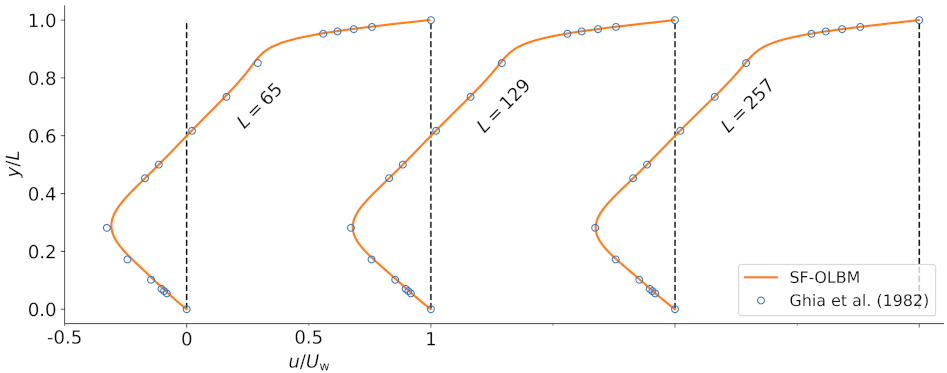
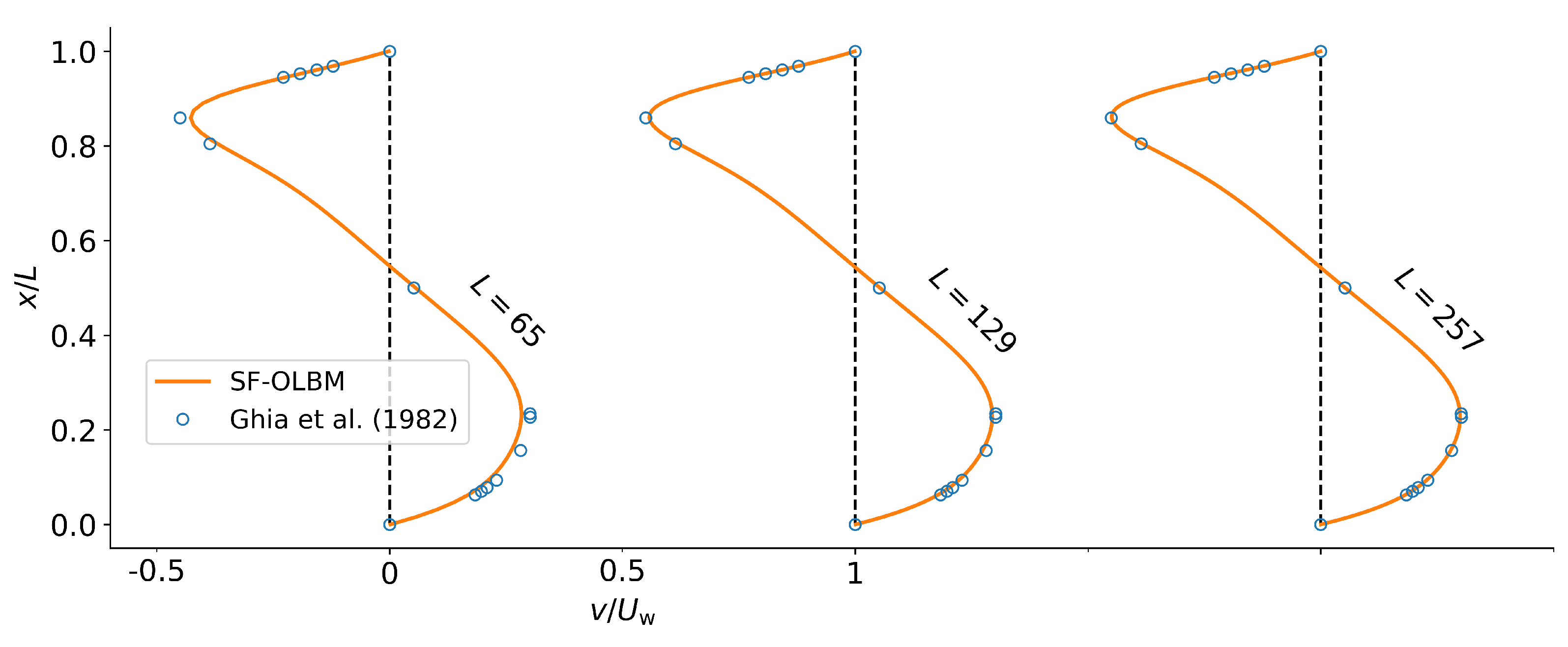
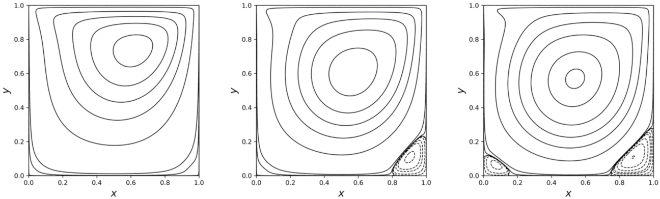
3.2. Lid-Driven Cavity Flow

The lid-driven cavity flow is a classic benchmark problem for numerical schemes in CFD. The popularity of this benchmark problem is due to its simple setup, consisting of a square cavity with side length L. The lid of the cavity moves with constant velocity U w , while the remaining walls are kept stationary. The Reynolds number of the flow is Re = U w L / ν with ν being the viscosity of the fluid. Although geometrically simple, the flow in the cavity is non-trivial, with the existence of thin boundary layers, and secondary vortices in the corners, that develop as the Reynolds number is increased. Moreover, a numerical singularity exists at the top corners of the cavity that can trigger the instability of the numerical scheme. Here, we use the lid-driven cavity flow to evaluate the spatial accuracy of the proposed OLBM at steady state and also to demonstrate the advantages of using irregular point clouds.

3.2.1. Spatial Accuracy on Regular Cartesian Grids

Here, we look at the spatial convergence of the SF-OLBM on a regular Cartesian grid. We use MLS including polynomials up to second order on 12-node nearest neighbor stencils. The settings are justified by the low error observed in the Taylor–Green benchmark (see Figure 4b). We fix the cavity length to L = 1 , CFL number to 0.1 and the ratio Δ t / τ = 5.1 . Calculations are performed for regular grids of size 65 × 65 , 129 × 129 , and 257 × 257 . The Reynolds number is set to Re = 400 , with the lid velocity fixed at U w = 1 , and viscosity ν = 0.025 . On the coarsest grid we set Ma = 0.05 and halve it with each increase in grid size by modifying the speed of sound c s . Although the Mach number varies, the set up corresponds to an acoustic scaling M a Δ t / Δ x .
Figure 6 shows the steady-state horizontal velocity profile along the vertical line through the center of the cavity for different grid sizes. The results are compared to the benchmark solutions of Ghia et al. [64] obtained by solving the Navier–Stokes equations. The OLBM results from the 129 × 129 grid are already in close agreement with the benchmark solutions. Analogously, the vertical velocity profiles along the horizontal center line are shown in Figure 7. Again, we observe good agreement with the benchmark results as the grid size is increased.
The flow pattern in the cavity can be visualized with the help of streamlines, that is, contours of the stream-function ψ . These can be obtained as the solution to the Poisson problem:
Δ ψ = ω ,
where Δ is the Laplace operator and ω = × u is the vorticity. The stream-function must also satisfy the homogeneous boundary conditions ψ = 0 at the four walls. Upon reaching steady-state, we use the pre-calculated derivative coefficients to set up a linear system of equations for the unknown stream-function values at the nodes, and calculate the vorticity values appearing on the right-hand side. The sparse system of equations is solved using the BiCGSTAB method available in the Eigen library.
The calculated stream functions for three different Reynolds number are displayed in Figure 8 and agree visually with previous results [28,63,64,65]. The calculations are performed using MLS approximation with second order polynomials on a 80 × 80 grid and a fixed CFL value of 0.8 (for Re = 1000 we use a CFL value of 0.4 ).

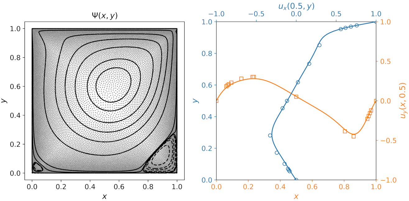
3.2.2. Irregular Point Cloud Calculation

One of the main benefits of the proposed OLBM is the opportunity to vary the density of the nodes in space. This means nodes can be placed in areas where they are needed, for example, boundary or internal layers. In standard LBM the grid spacing is constant, and determined by the smallest existing flow structures, meaning that the calculations are often over-resolved elsewhere. By varying the node density, we can achieve similar global accuracy with a smaller number of nodes. Unlike the multi-scale LBM, which uses a hierarchy of successively refined grids that demand specialized data structures, in the mesh-free setting we are able to use smoothly-varying nodes with practically no changes to the computational algorithm.
The actual point generation is performed using the fast point cloud generator of Slak and Kosec [60], followed by 100 steps of a relaxation procedure. The resulting point cloud with N = 16,298 nodes is shown in Figure 9. Each edge was discretized with 200 nodes; if a regular grid were used this would give a total of over 40,000 nodes, meaning a more than two-fold reduction was achieved. The RBF-FD stencil used the 21 nearest neighbors, quintic polyharmonic splines ( r 5 ) and polynomials up to second order. Calculations were performed for Re = 400 . The remaining parameters are chosen as Ma 0.04 and C F L = 0.1 .
The remaining mismatch between velocity cross-sections and benchmark results in Figure 9 (right) being attributed to the higher dissipation of irregular grids. This is obvious when compared with the Cartesian results from the N = 129 2 = 16,641 grid (see Figure 6 and Figure 7). A reduction in the amount of dissipation could be achieved with tuning of the RBF-FD (or MLS) approximations by including higher-order polynomials or changing the RBF (or weight function in MLS).

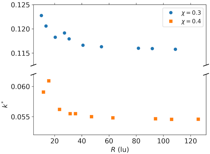
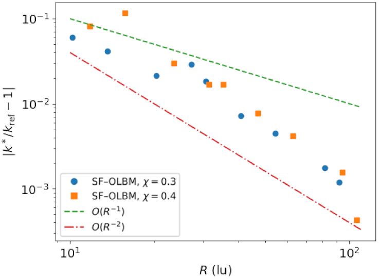
3.3. Flow over a Periodic Square Array of Cylinders

In this section, we study the boundary condition convergence behavior for Stokes flow through a periodic square array of cylinders. Similar benchmark computations have been used previously in [30,66,67] on lattice Boltzmann boundary conditions and the behavior of numerical error with bounce-back methods.
The set-up for this benchmark follows the descriptions in Refs. [67,68] and consists of a single cylinder of radius R in a square unit cell of length L. For the case of linear flow, analytic expressions are available for the dimensionless permeability k , defined such that the force per unit length of cylinder in the flowing medium is:
F = 4 π μ U ¯ k ,
where U ¯ is the average flow rate through the unit cell, and μ is the dynamic viscosity of the fluid. The dimensionless permeability k = k ( χ ) depends on the solid volume fraction χ = π R 2 / L 2 . Note that, at intermediate values of χ (e.g., between 0.2 and 0.5) away from the dilute ( χ 1 ) and lubrication-type ( χ χ max = π / 4 ) regimes, a small change in χ (or equivalently the radius of the cylinder) can lead to a ten-fold increase in hydrodynamic force, making this a sensitive test for the correctness of the implementation.
For simplicity, the average flow rate in Equation (21) is calculated as the volume average of velocity values in x-direction, that is,
U ¯ = 1 L 2 x u x ( x ) .
Note that the sum above is only a crude integration rule; better results can likely be obtained with more purposefully placed integration points. The force in Equation (21) contains contributions from a pure frictional force F D and a buoyancy force F B due to a pressure gradient. In the computations, the flow is driven instead by an external force b = ( b x , 0 ) and the buoyancy force is given by F B = π R 2 b x [30,69]. The drag and lift forces are obtainable from the the surface integral of traction along the cylinder boundary,
F D , F L = 0 2 π σ ( θ ) · n d θ ,
where σ ( θ ) is the stress tensor and n = ( cos θ , sin θ ) is the unit normal vector pointing from the surface into the fluid.
The stress tensor is a combination of the viscous stresses and an isotropic pressure part,
σ = σ + I ρ c s 2 .
In LBM, the viscous part of stress tensor σ = σ α β can be recovered from the non-equilibrium part of the distribution functions (up to third order) according to:
σ α β = 1 1 + Δ t / 2 τ i f ˜ i f i ( 0 ) c i α c i β .
Alternatively, the differentiation stencils can be used to compute σ = ν ρ 0 ( u + ( u ) T ) from the macroscopic velocity field. However, the use of Equation (25) is preferred due to the locality of the expression [70]. Together, Equations (21)–(24) can be reorganized to compute the dimensionless permeability explicitly as:
k = 4 π μ U ¯ F D + F B .
Unlike in regular LBM methods, where periodicity is enforced by simply reintroducing values exiting the domain on the opposite side, in the off-lattice method we enforce periodicity already during the construction of the derivative stencils and the calculation of weight coefficients. The point clouds are generated according to the method described in Section 2.4, starting from an initial set of nodes placed equidistantly on the cylinder’s surface. We use the TRT collision model [20] with τ = 4 / 5 and Λ = 1 / 4 . The body force is set to b x = 7.7 × 10 7 and lowered if necessary to assure creeping flow. Upon reaching steady state, the Reynolds number based upon the average velocity in x-direction, that is, Re = 2 R u x / ν and u x = x u x ( x ) / N , is checked to satisfy Re < 0.005 .
First, we increase the resolution of the cylinder at fixed values of the solid fraction χ { 0.3 , 0.4 } and measure the convergence of the dimensionless permeability k in terms of the relative error:
E ( k ) = k k ref 1 ,
with respect to a reference value k ref . The convergence of the dimensionless permeability with respect to the cylinder’s radius is displayed in Figure 10 and can be seen to approach a terminal value. Figure 11. shows the relative error (with respect to the value on the finest point cloud) as a function of the cylinder’s radius with logarithmic axes. The convergence rate is slightly below second order. The results for unit cells of size 33 2 , 99 2 , 297 2 , and 352 2 lattice units are given in Table 3. From these results we can see that, while the dimensionless permeability values are converged to the accuracy of three significant digits, a small error remains in comparison to the reference semi-analytical solution [68]. Part of this error is likely attributable to the integration errors when calculating the mean flow rate using the point sum over the irregularly distributed points. By interpolating the results onto a Cartesian grid akin to a standard LBM one we have calculated a second set of voxelized error values, where this effect is expected to be reduced. A cubic interpolation method was used in order to prevent interpolation errors from interfering with the LBM ones. The permeability values measured from the voxelized solution are in close agreement with the reference values obtained with standard LBM and the bounce-back boundary condition (see Table 3).
Further work is necessary to evaluate the other families of LBM boundary conditions in the off-lattice setting including least-squares and moment based approaches that are also applicable to higher order lattices. Advanced nodal integration methods should be sought to reduce the errors in averaged quantities such as permeability.

4. Conclusions

In this work, we have introduced a strong-form off-lattice Boltzmann method (SF-OLBM) based upon the Lax–Wendroff discretization in time and an RBF-FD or MLS discretization of the spatial terms. For static grids, the discretization weights only need to be computed once at the beginning of the calculation and stored as a sparse matrix for use in time-stepping. The second order accuracy of this approach when using PHS + poly RBF-FD on various stencils has been shown for the Taylor–Green vortex flow. Higher accuracy can be achieved by increasing the polynomial order of the approximations with a related increase in stencil size. The moving least squares approximations delivered good accuracy on Cartesian grids. For irregular points, the existence of a turn-over point was found where RBF-FD was able to perform better.
The ability to employ local point cloud refinement was demonstrated for the lid-driven cavity flow and could increase the global accuracy with little extra computational effort. For coarse grids in the presence of boundaries we found some errors in mass conservation, which however, disappear with increasing node density and high order approximations. The flow around a periodic square array of cylinders was used to probe the accuracy of the method in the presence of curved boundaries and raised the issue of computing accurate averaged quantities.
A downside of the proposed SF-OLBM, shared with other Eulerian lattice Boltzmann methods, is the loss of locality and large computational cost associated with the derivation evaluation in the streaming step. This decrease in efficiency can, however, be off-set using higher order approximations and local point cloud refinement. The opportunity to employ a high-level coordinate-free programming style is an additional benefit that saves on development time. A comparison of the current Lax–Wendroff streaming versus other streaming methods, including the semi-Lagrangian LBM [71] and the popular DUGKS scheme [29], remains a topic of future interest.

Author Contributions

Conceptualization: I.P.; methodology, I.P., T.B. and E.F.; coding, I.P. and E.F.; validation, I.P., T.B. and E.F.; formal analysis, I.P. and E.F.; investigation, I.P., T.B. and E.F.; data curation, I.P. and E.F.; writing–review and editing, I.P., T.B. and E.F.; visualization, I.P. and E.F. All authors have read and agreed to the published version of the manuscript.

Funding

Funded by the Deutsche Forschungsgemeinschaft (DFG, German Research Foundation)—Project number: BE 2245/15-1.

Institutional Review Board Statement

Not applicable.

Informed Consent Statement

Not applicable.

Data Availability Statement

Not applicable.

Conflicts of Interest

The authors declare no conflict of interest.

Abbreviations

The following abbreviations are used in this manuscript:
BGKBhatnagar-Gross-Krook
CFLCourant-Friedrichs-Lewy number
CPUcentral processing unit
DVBEdiscrete velocity Boltzmann equation
DVBMdiscrete velocity Boltzmann model
DUGKSdiscrete unified gas-kinetic method
FDMfinite difference method
FEMfinite element method
FVMfinite volume method
LBMlattice Boltzmann method
MLSmoving least squares
MRTmultiple-relaxation-time
OLBMoff-lattice Boltzmann method
PHSpolyharmonic spline
PDFparticle distribution function
RBF-FDradial basis function-generated finite differences
SF-OLBMstrong-form off-lattice Boltzmann method
TRTtwo-relaxation-time

References

  1. Qian, Y.H.; Succi, S.; Orszag, S. Recent advances in lattice Boltzmann computing. In Annual Reviews of Computational Physics III; World Scientific: Singapore, 1995; pp. 195–242. [Google Scholar]
  2. Chen, S.; Doolen, G.D. Lattice Boltzmann method for fluid flows. Annu. Rev. Fluid Mech. 1998, 30, 329–364. [Google Scholar] [CrossRef] [Green Version]
  3. Fattahi, E.; Waluga, C.; Wohlmuth, B.; Rüde, U. Large scale lattice Boltzmann simulation for the coupling of free and porous media flow. In Proceedings of the International Conference on High Performance Computing in Science and Engineering, Soláň, Czech Republic, 25–28 May 2015; pp. 1–18. [Google Scholar]
  4. Liu, H.; Kang, Q.; Leonardi, C.R.; Schmieschek, S.; Narváez, A.; Jones, B.D.; Williams, J.R.; Valocchi, A.J.; Harting, J. Multiphase lattice Boltzmann simulations for porous media applications. Comput. Geosci. 2016, 20, 777–805. [Google Scholar] [CrossRef] [Green Version]
  5. Fattahi, E.; Farhadi, M.; Sedighi, K. Lattice Boltzmann simulation of natural convection heat transfer in eccentric annulus. Int. J. Therm. Sci. 2010, 49, 2353–2362. [Google Scholar] [CrossRef]
  6. Fattahi, E.; Farhadi, M.; Sedighi, K.; Nemati, H. Lattice Boltzmann simulation of natural convection heat transfer in nanofluids. Int. J. Therm. Sci. 2012, 52, 137–144. [Google Scholar] [CrossRef]
  7. Sullivan, S.; Sani, F.; Johns, M.; Gladden, L. Simulation of packed bed reactors using lattice Boltzmann methods. Chem. Eng. Sci. 2005, 60, 3405–3418. [Google Scholar] [CrossRef]
  8. Aidun, C.K.; Clausen, J.R. Lattice-Boltzmann method for complex flows. Annu. Rev. Fluid Mech. 2010, 42, 439–472. [Google Scholar] [CrossRef]
  9. Succi, S.; Succi, S. The Lattice Boltzmann Equation: For Complex States of Flowing Matter; Oxford University Press: Oxford, UK, 2018. [Google Scholar]
  10. Godenschwager, C.; Schornbaum, F.; Bauer, M.; Köstler, H.; Rüde, U. A framework for hybrid parallel flow simulations with a trillion cells in complex geometries. In Proceedings of the International Conference on High Performance Computing, Networking, Storage and Analysis, Denver, CO, USA, 17–21 November 2013; pp. 1–12. [Google Scholar]
  11. Krüger, T.; Kusumaatmaja, H.; Kuzmin, A.; Shardt, O.; Silva, G.; Viggen, E.M. The Lattice Boltzmann Method; Springer International Publishing: Cham, Switzerland, 2017. [Google Scholar] [CrossRef]
  12. Bardow, A.; Karlin, I.V.; Gusev, A.A. General characteristic-based algorithm for off-lattice Boltzmann simulations. Europhys. Lett. 2006, 75, 434–440. [Google Scholar] [CrossRef]
  13. Körner, C.; Pohl, T.; Rüde, U.; Thürey, N.; Zeiser, T. Parallel lattice Boltzmann methods for CFD applications. In Numerical Solution of Partial Differential Equations on Parallel Computers; Springer: Berlin/Heidelberg, Germany, 2006; pp. 439–466. [Google Scholar]
  14. Dellar, P.J. Lattice Boltzmann algorithms without cubic defects in Galilean invariance on standard lattices. J. Comput. Phys. 2014, 259, 270–283. [Google Scholar] [CrossRef]
  15. Coreixas, C.; Wissocq, G.; Puigt, G.; Boussuge, J.F.; Sagaut, P. Recursive regularization step for high-order lattice Boltzmann methods. Phys. Rev. E 2017, 96, 033306. [Google Scholar] [CrossRef] [PubMed] [Green Version]
  16. Pavol, P.; Vahala, G.; Vahala, L. Higher Order Isotropic Velocity Grids in Lattice Methods. Phys. Rev. Lett. 1998, 80, 3960. [Google Scholar] [CrossRef] [Green Version]
  17. Malaspinas, O.; Chopard, B.; Latt, J. General regularized boundary condition for multi-speed lattice Boltzmann models. Comput. Fluids 2011, 49, 29–35. [Google Scholar] [CrossRef]
  18. Silva, G.; Semiao, V. Truncation errors and the rotational invariance of three-dimensional lattice models in the lattice Boltzmann method. J. Comput. Phys. 2014, 269, 259–279. [Google Scholar] [CrossRef]
  19. Wissocq, G.; Sagaut, P.; Boussuge, J.F. An extended spectral analysis of the lattice Boltzmann method: Modal interactions and stability issues. J. Comput. Phys. 2019, 380, 311–333. [Google Scholar] [CrossRef]
  20. Ginzburg, I.; Verhaeghe, F.; d’Humieres, D. Study of simple hydrodynamic solutions with the two-relaxation-times lattice Boltzmann scheme. Commun. Comput. Phys. 2008, 3, 519–581. [Google Scholar]
  21. Lallemand, P.; Luo, L.S. Theory of the lattice Boltzmann method: Dispersion, dissipation, isotropy, Galilean invariance, and stability. Phys. Rev. E 2000, 61, 6546. [Google Scholar] [CrossRef] [PubMed] [Green Version]
  22. Geier, M.; Schönherr, M.; Pasquali, A.; Krafczyk, M. The cumulant lattice Boltzmann equation in three dimensions: Theory and validation. Comput. Math. Appl. 2015, 70, 507–547. [Google Scholar] [CrossRef] [Green Version]
  23. Filippova, O.; Hänel, D. Grid refinement for lattice-BGK models. J. Comput. Phys. 1998, 147, 219–228. [Google Scholar] [CrossRef]
  24. Filippova, O.; Hänel, D. Acceleration of lattice-BGK schemes with grid refinement. J. Comput. Phys. 2000, 165, 407–427. [Google Scholar] [CrossRef]
  25. Lagrava, D.; Malaspinas, O.; Latt, J.; Chopard, B. Advances in multi-domain lattice Boltzmann grid refinement. J. Comput. Phys. 2012, 231, 4808–4822. [Google Scholar] [CrossRef] [Green Version]
  26. Eitel-Amor, G.; Meinke, M.; Schröder, W. A lattice-Boltzmann method with hierarchically refined meshes. Comput. Fluids 2013, 75, 127–139. [Google Scholar] [CrossRef]
  27. Reider, M.B.; Sterling, J.D. Accuracy of discrete-velocity BGK models for the simulation of the incompressible Navier-Stokes equations. Comput. Fluids 1995, 24, 459–467. [Google Scholar] [CrossRef] [Green Version]
  28. Lee, T.; Lin, C.L. A Characteristic Galerkin Method for Discrete Boltzmann Equation. J. Comput. Phys. 2001, 171, 336–356. [Google Scholar] [CrossRef]
  29. Guo, Z.; Xu, K.; Wang, R. Discrete unified gas kinetic scheme for all Knudsen number flows: Low-speed isothermal case. Phys. Rev. E 2013, 88, 033305. [Google Scholar] [CrossRef] [PubMed] [Green Version]
  30. Fattahi, E.; Waluga, C.; Wohlmuth, B.; Rüde, U.; Manhart, M.; Helmig, R. Lattice Boltzmann methods in porous media simulations: From laminar to turbulent flow. Comput. Fluids 2016, 140, 247–259. [Google Scholar] [CrossRef]
  31. Coreixas, C.; Chopard, B.; Latt, J. Comprehensive comparison of collision models in the lattice Boltzmann framework: Theoretical investigations. Phys. Rev. E 2019, 100, 033305. [Google Scholar] [CrossRef] [PubMed] [Green Version]
  32. Bauer, M.; Silva, G.; Rüde, U. Letter to the Editor: Truncation errors of the D3Q19 lattice model for the lattice Boltzmann method. J. Comput. Phys. 2019, 405, 109111. [Google Scholar] [CrossRef]
  33. Schornbaum, F.; Rüde, U. Extreme-Scale Block-Structured Adaptive Mesh Refinement. SIAM J. Sci. Comput. 2018, 40, C358–C387. [Google Scholar] [CrossRef] [Green Version]
  34. Bardow, A.; Karlin, I.V.; Gusev, A.A. Multispeed models in off-lattice Boltzmann simulations. Phys. Rev. E 2008, 77, 025701. [Google Scholar] [CrossRef] [Green Version]
  35. Chen, H.; Goldhirsch, I.; Orszag, S.A. Discrete rotational symmetry, moment isotropy, and higher order lattice Boltzmann models. J. Sci. Comput. 2008, 34, 87–112. [Google Scholar] [CrossRef]
  36. McCracken, M.E.; Abraham, J. Lattice Boltzmann methods for binary mixtures with different molecular weights. Phys. Rev. E 2005, 71, 046704. [Google Scholar] [CrossRef]
  37. Lin, C.; Luo, K.H.; Fei, L.; Succi, S. A multi-component discrete Boltzmann model for nonequilibrium reactive flows. Sci. Rep. 2017, 7, 14580. [Google Scholar] [CrossRef] [PubMed]
  38. Horstmann, J.T.; Le Garrec, T.; Mincu, D.C.; Lévêque, E. Hybrid simulation combining two space–time discretization of the discrete-velocity Boltzmann equation. J. Comput. Phys. 2017, 349, 399–414. [Google Scholar] [CrossRef]
  39. Krämer, A.; Küllmer, K.; Reith, D.; Joppich, W.; Foysi, H. Semi-Lagrangian off-lattice Boltzmann method for weakly compressible flows. Phys. Rev. E 2017, 95, 023305. [Google Scholar] [CrossRef] [PubMed]
  40. Wu, C.; Shi, B.; Shu, C.; Chen, Z. Third-order discrete unified gas kinetic scheme for continuum and rarefied flows: Low-speed isothermal case. Phys. Rev. E 2018, 97, 023306. [Google Scholar] [CrossRef] [Green Version]
  41. Krämer, A.; Wilde, D.; Küllmer, K.; Reith, D.; Foysi, H.; Joppich, W. Lattice Boltzmann simulations on irregular grids: Introduction of the NATriuM library. Comput. Math. Appl. 2020, 79, 34–54. [Google Scholar] [CrossRef]
  42. Succi, S.; Nannelli, F. The finite volume formulation of the Lattice Boltzmann equation. Transp. Theory Stat. Phys. 1994, 23, 163–171. [Google Scholar] [CrossRef]
  43. Guo, Z.; Zhao, T.S. Explicit finite-difference lattice Boltzmann method for curvilinear coordinates. Phys. Rev. E 2003, 67, 066709. [Google Scholar] [CrossRef]
  44. Li, Y.; LeBoeuf, E.J.; Basu, P.K. Least-squares finite-element lattice Boltzmann method. Phys. Rev. E 2004, 69, 065701. [Google Scholar] [CrossRef] [Green Version]
  45. He, X.; Chen, S.; Doolen, G.D. A novel thermal model for the lattice Boltzmann method in incompressible limit. J. Comput. Phys. 1998, 146, 282–300. [Google Scholar] [CrossRef]
  46. Dellar, P.J. An interpretation and derivation of the lattice Boltzmann method using Strang splitting. Comput. Math. Appl. 2013, 65, 129–141. [Google Scholar] [CrossRef]
  47. Shu, C.; Niu, X.D.; Chew, Y.T. Taylor-series expansion and least-squares-based lattice Boltzmann method: Two-dimensional formulation and its applications. Phys. Rev. E 2002, 65, 036708. [Google Scholar] [CrossRef] [Green Version]
  48. Bayona, V. Comparison of moving least squares and RBF+poly for interpolation and derivative approximation. J. Sci. Comput. 2019, 81, 486–512. [Google Scholar] [CrossRef]
  49. Musavi, S.H.; Ashrafizaadeh, M. Meshless lattice Boltzmann method for the simulation of fluid flows. Phys. Rev. E 2015, 91, 023310. [Google Scholar] [CrossRef]
  50. Musavi, H.S.; Ashrafizaadeh, M. A mesh-free lattice Boltzmann solver for flows in complex geometries. Int. J. Heat Fluid Flow 2016, 59, 10–19. [Google Scholar] [CrossRef]
  51. Tanwar, S. A Meshfree-Based Lattice Boltzmann Approach for Simulation of Fluid Flows Within Complex Geometries: Application of Meshfree Methods for LBM Simulations. In Analysis and Applications of Lattice Boltzmann Simulations; IGI Global: Hershey, PA, USA, 2018. [Google Scholar] [CrossRef]
  52. Dellar, P.J. Incompressible limits of lattice Boltzmann equations using multiple relaxation times. J. Comput. Phys. 2003, 190, 351–370. [Google Scholar] [CrossRef] [Green Version]
  53. Gorakifard, M.; Salueña, C.; Cuesta, I.; Far, E.K. Analysis of Aeroacoustic Properties of the Local Radial Point Interpolation Cumulant Lattice Boltzmann Method. Energies 2021, 14, 1443. [Google Scholar] [CrossRef]
  54. Trobec, R.; Kosec, G. Parallel Scientific Computing: Theory, Algorithms, and Applications of Mesh Based and Meshless Methods; Springer: Berlin/Heidelberg, Germany, 2015. [Google Scholar]
  55. Fornberg, B.; Flyer, N. A Primer on Radial Basis Functions with Applications to the Geosciences; Society for Industrial and Applied Mathematics: Philadelphia, PA, USA, 2015. [Google Scholar]
  56. Slak, J.; Kosec, G. Medusa: A C++ Library for Solving PDEs Using Strong Form Mesh-Free Methods. ACM Trans. Math. Softw. 2021, 47, 1–25. [Google Scholar] [CrossRef]
  57. Malaspinas, O. Increasing stability and accuracy of the lattice Boltzmann scheme: Recursivity and regularization. arXiv 2015. [Google Scholar]
  58. Fornberg, B.; Flyer, N. Fast generation of 2-D node distributions for mesh-free PDE discretizations. Comput. Math. Appl. 2015, 69, 531–544. [Google Scholar] [CrossRef]
  59. Zamolo, R.; Nobile, E. Two algorithms for fast 2D node generation: Application to RBF meshless discretization of diffusion problems and image halftoning. Comput. Math. Appl. 2018, 75, 4305–4321. [Google Scholar] [CrossRef]
  60. Slak, J.; Kosec, G. On generation of node distributions for meshless PDE discretizations. SIAM J. Sci. Comput. 2019, 41, A3202–A3229. [Google Scholar] [CrossRef] [Green Version]
  61. Bayona, V.; Flyer, N.; Fornberg, B.; Barnett, G.A. On the role of polynomials in RBF-FD approximations: II. Numerical solution of elliptic PDEs. J. Comput. Phys. 2017, 332, 257–273. [Google Scholar] [CrossRef] [Green Version]
  62. Flyer, N.; Fornberg, B.; Bayona, V.; Barnett, G.A. On the role of polynomials in RBF-FD approximations: I. Interpolation and accuracy. J. Comput. Phys. 2016, 321, 21–38. [Google Scholar] [CrossRef] [Green Version]
  63. Zhu, L.; Wang, P.; Guo, Z. Performance evaluation of the general characteristics based off-lattice Boltzmann scheme and DUGKS for low speed continuum flows. J. Comput. Phys. 2017, 333, 227–246. [Google Scholar] [CrossRef] [Green Version]
  64. Ghia, U.; Ghia, K.N.; Shin, C. High-Re solutions for incompressible flow using the Navier-Stokes equations and a multigrid method. J. Comput. Phys. 1982, 48, 387–411. [Google Scholar] [CrossRef]
  65. Hou, S.; Zou, Q.; Chen, S.; Doolen, G.; Cogley, A.C. Simulation of cavity flow by the lattice Boltzmann method. J. Comput. Phys. 1995, 118, 329–347. [Google Scholar] [CrossRef] [Green Version]
  66. Bouzidi, M.; Firdaouss, M.; Lallemand, P. Momentum transfer of a Boltzmann-lattice fluid with boundaries. Phys. Fluids 2001, 13, 3452–3459. [Google Scholar] [CrossRef]
  67. Ginzburg, I.; d’Humières, D. Multireflection boundary conditions for lattice Boltzmann models. Phys. Rev. E 2003, 68, 066614. [Google Scholar] [CrossRef] [PubMed] [Green Version]
  68. Sangani, A.S.; Acrivos, A. Slow flow past periodic arrays of cylinders with application to heat transfer. Int. J. Multiph. Flow 1982, 8, 193–206. [Google Scholar] [CrossRef]
  69. Bogner, S. Direkte Numerische Simulation von Flüssig-Gas-Feststoff-Strömungen Basierend auf der Lattice Boltzmann-Methode. Ph.D. Thesis, University of Erlangen-Nuremberg, Erlangen, Germany, 2017. [Google Scholar]
  70. Di Ilio, G.; Chiappini, D.; Ubertini, S.; Bella, G.; Succi, S. Hybrid lattice Boltzmann method on overlapping grids. Phys. Rev. E 2017, 95, 013309. [Google Scholar] [CrossRef]
  71. Krämer, A. Lattice-Boltzmann-Methoden zur Simulation Inkompressibler Wirbelströmungen. Ph.D. Thesis, Universität Siegen, Siegen, Germany, 2017. [Google Scholar]
Figure 1. Scattered point set produced by Poisson disk sampling followed by an annealing process.
Symmetry 13 01802 g001
Figure 2. Cartesian (a) and scattered (b) node distributions ( L = L 0 = 32 ) used in the spatial convergence studies of the Taylor–Green vortex flow benchmark. The (target) inter-nodal spacing is h = 1 . Example stencils of the 21 nearest neighbors (including the point itself) are marked with orange circles. (For colors please see online publication).
Symmetry 13 01802 g002
Figure 3. Error with respect to N for Cartesian point cloud (C), (left) viscosity error, (right) velocity error. Dashed line indicates slope proportional to 1 / N .
Symmetry 13 01802 g003
Figure 4. Error with respect to N for scattered point cloud (S), (left) viscosity error, (right) velocity error. Dashed line indicates slope proportional to 1 / N .
Symmetry 13 01802 g004
Figure 5. Comparison of SF-OLBM with the methods of Bardow and DUGKS. (left) Spatial accuracy for grids of size 16 2 , 32 2 , 64 2 , and 128 2 ; dashed line indicates slope proportional to 1 / N . (right) Temporal accuracy for varying Δ t / τ ; dashed line indicates slope proportional to Δ t . Due to error incurred during extraction from the original figure, the Bardow and DUGKS values near the abscissae Δ t / τ = 1 and Δ t / τ = 2 should be taken with caution.
Symmetry 13 01802 g005
Figure 6. Horizontal velocity profiles along the vertical center line of the cavity at Re = 400 .
Symmetry 13 01802 g006
Figure 7. Vertical velocity profiles along the horizontal center line of the cavity at Re = 400 .
Symmetry 13 01802 g007
Figure 8. Streamlines of the lid-driven cavity flow at Reynolds numbers. From left to right are Re = 100, 400, and 1000. The contour values of the stream function ψ are the same as those in [64].
Symmetry 13 01802 g008
Figure 9. Lid-driven cavity flow with irregular point cloud at Re = 400 . (left) Streamlines and underlying point cloud; (right) vertical (orange) and horizontal (blue) velocity along the mid-axes and their comparison to the benchmark results of Ghia et al. [64]. (For reference to color, please see online publication).
Symmetry 13 01802 g009
Figure 10. Convergence of the dimensionless permeability with respect to the cylinder radius for domains of size 33 2 , 44 2 , 66 2 , 88 2 , 99 2 , 132 9 , 176 2 , 264 2 , 297 2 , and 352 2 .
Symmetry 13 01802 g010
Figure 11. Convergence of the relative error in dimensionless permeability with respect to the cylinder radius for domains of size 33 2 , 44 2 , 66 2 , 88 2 , 99 2 , 132 9 , 176 2 , 264 2 , and 297 2 . The reference value k ref was as the value from obtained on the finest point cloud (domain size 352 2 ).
Symmetry 13 01802 g011
Table 1. Details of the approximations functions used for the spatial convergence evaluation. For the MLS approximants, the weight functions were scaled to the nearest neighbor.
AbbreviationWeightRBFMonomialsStencil Size
RBF-FD s9 r 3 1 , x , y , x 2 , x y , y 2 9
RBF-FD s13 r 3 1 , x , y , x 2 , x y , y 2 13
RBF-FD s21 r 3 1 , x , y , x 2 , x y , y 2 21
MLS s9Gaussian 1 , x , y , x 2 , x y , y 2 9
MLS s13Gaussian 1 , x , y , x 2 , x y , y 2 13
MLS s21Gaussian 1 , x , y , x 2 , x y , y 2 21
Table 2. Computation time in seconds for 10,000 time steps. Each value represents the average of five runs.
Grid Size\Stencil Size91321
64 × 64 2.93.55.0
128 × 128 13.817.024.9
Table 3. Comparison of dimensionless permeability values for a square array of cylinders and the proposed OLBM on 33 2 , 99 2 , 297 2 , and 352 2 sized domains discretized with scattered points. The results are compared to the solution in Ref. [68] (Table 1, p. 196) and values from Ref. [67] (Table VI, p. 13) obtained with standard LBM and half-way bounceback boundary conditions on a 99 2 grid.
332 Grid992 Grid2972 Grid3522 GridSemi-Analytic [68]LBM [67]
χ U ¯ x k U ¯ x k U ¯ x k U ¯ x k k k
Nodal average
0.35.1561 (−8)0.122774.8166 (−7)0.117934.3671 (−6)0.115936.1393 (−6)0.11579
0.42.8141 (−8)0.059072.6303 (−7)0.055502.4004 (−6)0.054563.3797 (−6)0.05458
Voxelized
0.33.8299 (−8)0.122613.4311 (−7)0.121153.0800 (−6)0.120804.3259 (−6)0.120790.122100.12121
0.41.8533 (−8)0.059301.6220 (−7)0.057321.4544 (−6)0.056862.0427 (−6)0.056760.057670.05684
Publisher’s Note: MDPI stays neutral with regard to jurisdictional claims in published maps and institutional affiliations.

