Closed-Form Solution of Adiabatic Particle Trajectories in Axis-Symmetric Magnetic Fields

Abstract

The dynamics of a low-energy charged particle in an axis-symmetric magnetic field is known to be a regular superposition of periodic—although possibly incommensurate—motions. The projection of the particle orbit along the two non-ignorable coordinates $(x,y)$ may be expressed in terms of each other: $y=y\left(x\right)$, yet—to our knowledge—such a functional relation has never been directly produced in literature, but only by way of a detour: first, equations of motion are solved, yielding $x=x\left(t\right),y=y\left(t\right)$, and then one of the two relations is inverted, $x\left(t\right)\to t\left(x\right)$. In this paper, we present a closed-form functional relation which allows us to express coordinates of the particle’s orbit without the need to pass through the hourly law of motion.

1. Introduction

In magnetized plasma research, it is fundamental to have knowledge of the particles’ trajectories moving within the magnetic fields; both in natural systems, and even more in laboratory systems. In nuclear fusion devices, confinement of the plasma is a critical issue, and it is crucial to design magnetic geometries which do not lead to particle losses to the walls of the device.

A charged particle moving in a given magnetic field, as long as we may neglect Coulomb collisions, is an instance of a Hamiltonian system, with Hamiltonian

$$H=\sum _i\frac{{(p_i-Q{A}_i\left(\mathbf{q}\right))}^2}{2M}$$

(1)

where $A_i$ are the components of the vector potential, $q_i$ the coordinate, $p_i$ the momenta, and $Q,M$ the particle’ charge and mass. Accordingly, one may exploit the vast knowledge accumulated in the theory of Hamiltonian systems in order to gain information about the particle behaviour. In particular, the existence of any symmetry in the system (1) is equivalent to a conservation law, and any conserved quantity constrains the flow within a restricted region of the whole phase-space $(q_i,p_i)$. In a three-dimensional system, the existence of three independent conserved quantities is sufficient to ensure that the trajectories are regular.

Laboratory devices for the study of magnetized plasma usually have the geometry of tori in the real space. Quite often, they are endowed with some sort of symmetry, too: either axis-symmetric, i.e., invariant with respect to rotations along the major circumference of the torus; or helically symmetrical, i.e., the system depends only upon the helical angle $\xi$, linear combination of the azimuthal and toroidal angles $\theta ,\varphi$, rather than from the two angles separately. In this work, we will consider the first case. In the following, for clarity, we will use the toroidal set of coordinates $(R,Z,\varphi )$, where $\varphi$ is the angle along the major circumference and the direction of symmetry, R the major radius, and Z the vertical axis. The axis-symmetry along $\varphi$ translates into the conservation of the conjugate momentum $p_{\varphi }$. In stationary magnetic fields, the total energy K is another conserved quantity, too.

This is as far as we can go with exact results. However, adiabatic invariants are to be considered, as well. Adiabatic invariants in a Hamiltonian system are phase space quantities, closely related to perturbed KAM tori, that stay constant while the system parameters are changed slowly. They were first introduced in the old quantum theory in order to decide which dynamical variables should be quantized. Later on, they appeared in purely classical settings: geophysics, astrophysics and the physics of strongly magnetized plasmas, in particular in connection with nuclear fusion. See the reviews [1,2] for an overview on the subject.

Each adiabatic invariant I is associated to a periodic motion in the phase space: $I=\oint pdq$, where $q,p$ are the usual coordinate and momentum. By introducing a slow perturbation to the Hamiltonian, the motion is no longer exactly periodic, yet I remains unchanged. For a charged particle in a magnetic field, the most intuitive and generic periodic motion is associated to the Larmor gyration around a magnetic field line, and the corresponding adiabatic invariant is the magnetic moment $\mu$ which, to leading order, writes $\mu =m{v}_{\perp }^2/\left(2B\right)$, where $v_{\perp }$ is the particle velocity perpendicular to the magnetic field $\mathbf{B}$ (Rigorously, $\mu$ is constant, but for a tiny component which oscillates with the Larmor frequency, if B is not exactly constant, and which is dropped out by averaging over one Larmor period. We will return to it later).

Conservation of the magnetic moment relies upon the postulate of a wide separation between the length and frequency scales of the individual particle motion $\rho$ (Larmor radius), $\mathsf{\Omega }$ (cyclotron frequency) and the analogous typical scales referring to the equilibrium magnetic field, $L,\omega$:

$$\rho /L,\omega /\mathsf{\Omega }\ll 1.$$

(2)

In laboratory plasmas, and often in astrophysical contexts, where a strong guiding magnetic field exists, this scale separation is generally satisfied by a wide margin.

In conclusion, endowed with the three conserved quantities $K,P_{\varphi },\mu$, we may claim that a charged particle in stationary axis-symmetric magnetic fields does follow regular orbits. Yet, one still has to actually produce the orbits. This is accomplished by integrating the equations of motion: either the exact Hamilton equations of motion derived from (1), or the guiding-center equations [3]. In the first case, the existence of conserved quantities does not explicitly enter the equations: it is a constraint which needs to be checked a posteriori in order to ensure the accuracy of the numerical solutions. Guiding centre equations, conversely, include in their structure from the outset the information about conserved quantities. In either case, one is eventually left with solutions in the form $R,Z,\varphi =R,Z,\varphi (\mathcal{C},t)$, where $\mathcal{C}$ collectively labels all the conserved quantities, and t is the time. These functional relations yield the hourly law with which orbits are travelled. It may happen that one will be interested in just the geometrical shape of the orbit, not to the rate at which it is travelled by the particle; i.e., not to $R\left(t\right),Z\left(t\right)$ separately, but in the $Z\left(R\right)$ relation (we do not consider the $\varphi$ coordinate, since it is physically less relevant). This can obviously be achieved by inverting the functional relation $R=R\left(t\right)\to t=t\left(R\right)$, and using R in place of t in the other law of motion: $Z\left(t\right)\to Z\left(R\right)$. In doing so, we feel like we are performing an unnecessary step: we have produced all the information about the temporal behaviour of the system, but eventually we do not really use it. With present-day computers, integrating systems of differential equations even over long times is not a serious concern, but one could, all the same, wonder whether it is really a necessary task; that is, if it possible to arrive to the $Z=Z\left(R\right)$ relation without passing throughout the intermediate step of computing their time evolution. Using the language of Hamiltonian systems, we wish to find a part of the canonical transformation from coordinates to action-angle variables: not the whole six-dimensional map, rather just the part that involves both $R,Z$ and the actions. To the best of our knowledge, this question does not seem to have ever been addressed in literature. The purpose of this work is precisely to do that: we will show that it is possible to write down the functional relation $R=R\left(Z\right)$ in closed form as an implicit equation $f(K,p_{\varphi },\mu ,R,Z)=0$, without the need of passing through the time integration of the equations of motion.

2. Derivation of the Z(R) Functional Relation

We write the magnetic potential $\mathbf{A}=(A_R,A_Z,A_{\varphi })$ in the gauge where $A_R=0$: $A_Z,A_{\varphi }=A_Z(R,Z),A_{\varphi }(R,Z)$. The magnetic field is computed as: $\mathbf{B}=\nabla \times \mathbf{A}$. For the sake of simplicity, we will consider normalized units $Q=M=1$.

Accordingly, Hamiltonian (1) writes

$$H=\frac{p_R^2}{2}+\frac{{(p_Z-A_Z)}^2}{2}+\frac{{(p_{\varphi }-A_{\varphi })}^2}{2}$$

(3)

We recall that the physical velocity is related to the momentum by $v_i=p_i-A_i$. In particular, $v_{\varphi }=p_{\varphi }-A_{\varphi }$.

Let us split the total kinetic energy into the part due to the motion along $\varphi$ and that perpendicular to it;

$$K_{RZ}=K-\frac{v_{\varphi }^2}{2}=\frac{v_R^2}{2}+\frac{v_Z^2}{2}$$

(4)

and define $v_R,v_Z$ in terms of new parameters $(w,\theta )$:

$$v_R=wcos\left(\theta \right),v_Z=wsin\left(\theta \right),w^2=2K_{RZ}$$

(5)

The velocity parallel to the magnetic field is

$$v_{\Vert }=\frac{v_R{B}_R+v_Z{B}_Z+v_{\varphi }{B}_{\varphi }}{B},B=\sqrt{B_R^2+B_Z^2+B_{\varphi }^2}$$

(6)

The part of the kinetic energy perpendicular to the magnetic field is

$$K_{\perp }=K-\frac{v_{\Vert }^2}{2}$$

(7)

The instantaneous magnetic moment thus writes

$$\mu =\frac{K_{\perp }}{B}$$

(8)

By using (4)–(7) into (8) we finally arrive to

$$\mu =\frac{K}{B}-\frac{{\left[B_{\varphi }(p_{\varphi }-A_{\varphi })+\sqrt{2K-{(p_{\varphi }-A_{\varphi })}^2}(B_{R}cos\left(\theta \right)+B_{Z}sin\left(\theta \right))\right]}^2}{2B^3}$$

(9)

We remind that still a tiny component oscillating at the Larmor frequency has to be removed from $\mu$. We make it explicit by writing $\mu =\langle \mu \rangle +\delta \mu \left(t\right)$.

Let us inspect the right hand side of (9): all quantities therein are either constant $(K,p_{\varphi })$, or depend upon $R,Z$ coordinates ($A_{\varphi },B$), or depend upon the parameter $\theta$. In the course of a Larmor gyration, the particle suffers a maximum displacement of the order of the Larmor radius; since we posited the validity of Equation (2), i.e., ${\rho }_L/L\ll 1$, all quantities depending upon $(R,Z)$ remain almost constant throughout one Larmor radius. The only quantity which may, therefore, vary periodically is $\theta$. This fact may be easily appreciated if the magnetic field is aligned along axis $\varphi$: $\theta$ is just the phase of the Larmor rotation around the local line field, i.e., $\theta =\mathsf{\Omega }t$, with $\mathsf{\Omega }=B$ the cyclotron frequency: it is the angle conjugate to the $\mu$ action. When the field is no longer aligned with $\varphi$, the phase is changed by small corrections depending by $v_{\varphi }$ and the magnetic field itself, which may be neglected to leading order.

We thus get rid of $\theta$ in Equation (9) by averaging upon a Larmor rotation, i.e., over $\theta$ varying between 0 and $2\pi$. This makes the $\delta \mu$ term to drop out in its left hand side, and the final result is

$$\langle \mu \rangle =\frac{K}{B}-\frac{1}{4B^3}\left[2B_{\varphi }^2{(p_{\varphi }-A_{\varphi })}^2+(B_R^2+B_Z^2)(2K-{(p_{\varphi }-A_{\varphi })}^2)\right]$$

(10)

This equation represents the sought functional relation involving $R,Z$, as well as all the conserved quantities $K,p_{\varphi },\mu$.

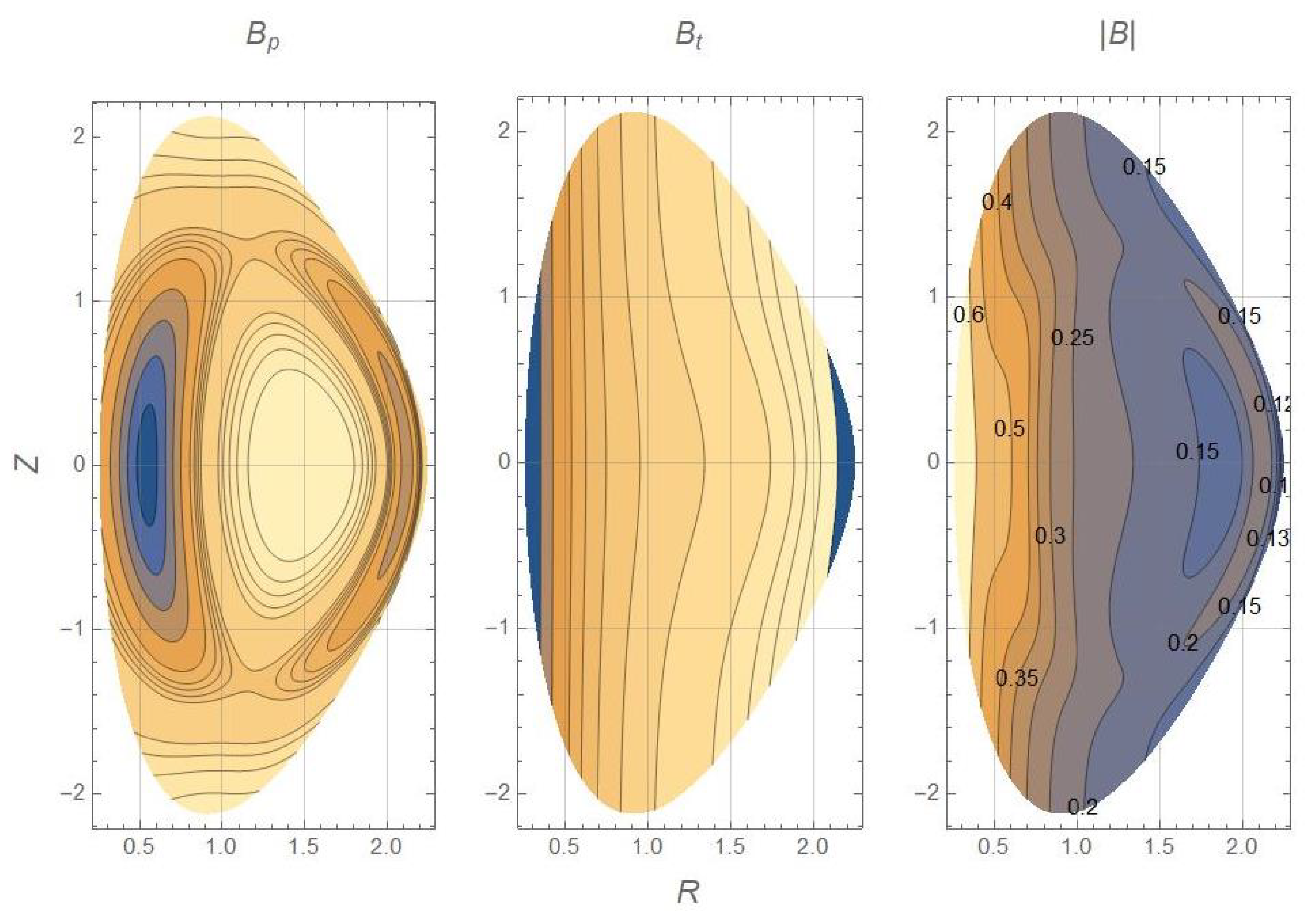
For didactical purposes, we shall apply Equation (10) to a realistic case: the map of the magnetic field produced in an axis-symmetric version of the NSTX spherical tokamak [4], as parameterized by [5] and implemented in [6]. We plot in Figure 1, for reference, the contour plots of the magnetic field. We point out, to this regard, a tricky issue: in actual cases, one usually works directly with the magnetic field, whereas Equation (10) involves the magnetic potential—as is natural since it has been derived within the framework of Hamiltonian dynamics, where the important quantities are the potentials, not the fields. Recovering the potential $\mathbf{A}$ from the field $\mathbf{B}$ may be not a simple exercise, and is the price to be paid for the simplicity of Equation (10); details about the procedure employed in this case have been described elsewhere [6] and shall not be repeated here.

The particles trajectories are computed by integrating Hamilton’s equations of motion with the symplectic partitioned Runge–Kutta algorithm of sixth order described in [7]. We initialized particles with a low kinetic energy; their Larmor radius turns out about $1\%$ of the minor radius. This does not ensure automatically that $\rho /L$ is small, since the analysis produced in [6] shows that there are regions where L is substantially smaller than the minor radius. However, for the specific trajectory that we are considering, we are confident that the motion is adiabatic. 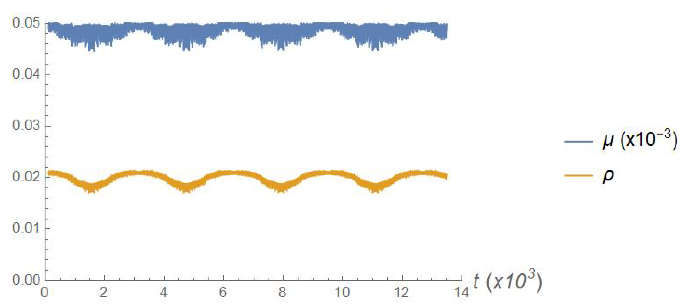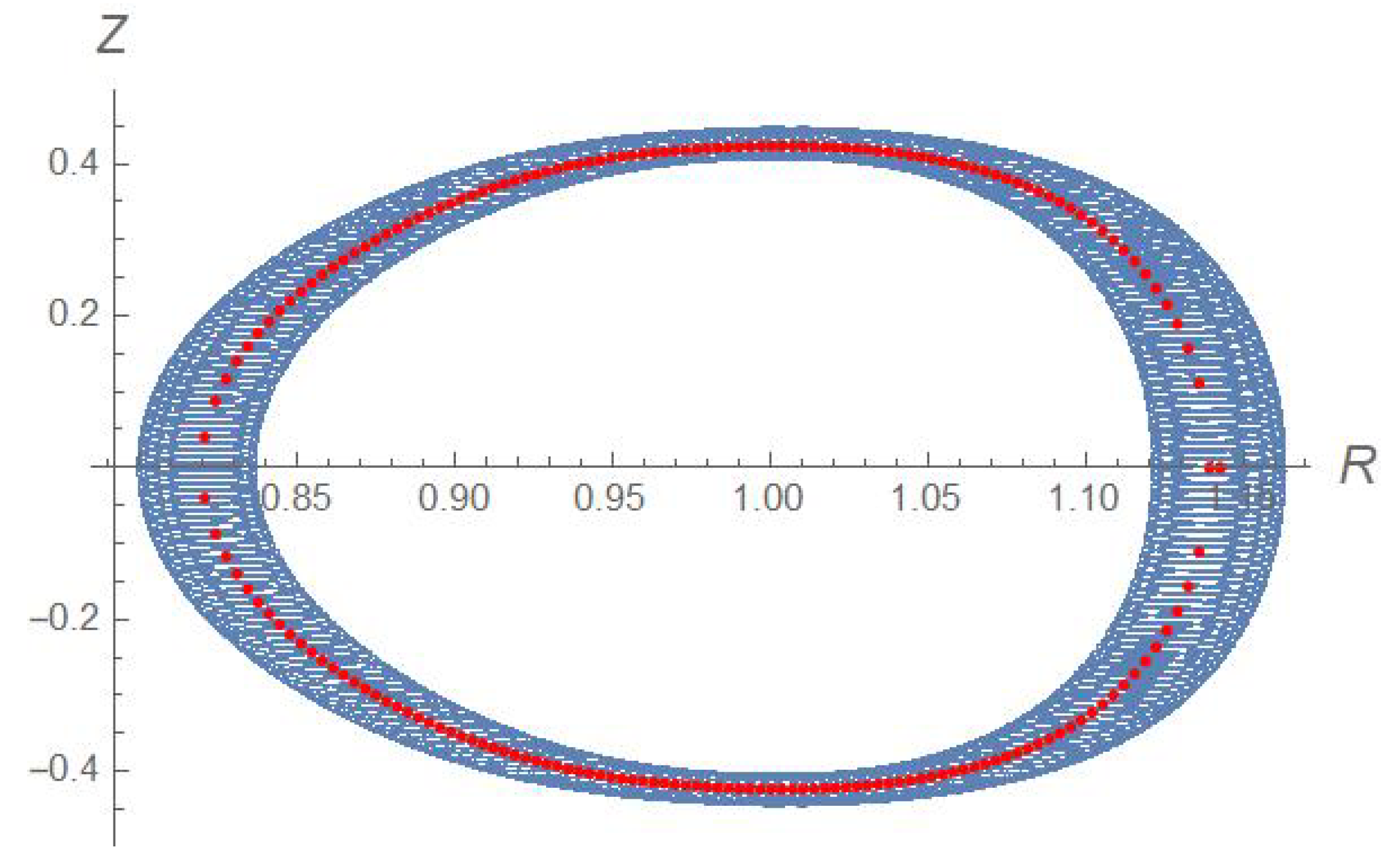Figure 2 shows a part of the time trace of the computed magnetic moment: it is clearly constant to a great degree. In Figure 3, finally we produce an example of the $(R,Z)$ projection of the trajectory. The blue dots are the numerically integrated full trajectory; the red dots are the solutions of Equation (10) which, by construction, coincide with the guiding centre coordinates. The two sets of points clearly overlap fairly well.

3. Summary

We have presented here a simple recipe for obtaining charged particle trajectories in axis-symmetric magnetic fields in closed form, provided that the adiabatic invariant magnetic moment is conserved, which is the case in most common scenarios, where the ratio (Larmor radius)/(length scale of the background field) is $\ll 1$.