US Dollar/Turkish Lira Exchange Rate Forecasting Model Based on Deep Learning Methodologies and Time Series Analysis

Abstract

Exchange rate forecasting has been an important topic for investors, researchers, and analysts. In this study, financial sentiment analysis (FSA) and time series analysis (TSA) are proposed to form a predicting model for US Dollar/Turkish Lira exchange rate. For this purpose, the proposed hybrid model is constructed in three stages: obtaining and modeling text data for FSA, obtaining and modeling numerical data for TSA, and blending two models like a symmetry. To our knowledge, this is the first study in the literature that uses social media platforms as a source for FSA and blends them with TSA methods. To perform FSA, word embedding methods Word2vec, GloVe, fastText, and deep learning models such as CNN, RNN, LSTM are used. To the best of our knowledge, this study is the first attempt in terms of performing the FSA by using the combinations of deep learning models with word embedding methods for both Turkish and English texts. For TSA, simple exponential smoothing, Holt–Winters, Holt’s linear, and ARIMA models are employed. Finally, with the usage of the proposed model, any user who wants to make a US Dollar/Turkish Lira exchange rate forecast will be able to make a more consistent and strong exchange rate forecast.

1. Introduction

Today, social networks have taken an important place in our daily lives. Users evaluate their free time using social platforms such as Twitter, Facebook, or Instagram. Although these habits are viewed negatively, the continued use of social media platforms by millions of people has become a research area and data source for researchers. The main reason for this is that the data are produced on these platforms in different types, such as pictures, text, and videos, in large volumes by millions of people at the same time very quickly. What distinguishes Twitter from other platforms is the size of its text-based data and the fact that it hosts more than 500 million observations of content daily. In addition, an average of 6000 content posts per second are published by users each day, and about 326 million users are active each month, making Twitter one of the most popular social media platforms worldwide. This ensures that Twitter remains fresh, large, and diverse at any moment. Moreover, Twitter is preferred as a true source of data not only by users’ own content but also by the variety of data generated by interacting with different users. Therefore, researchers or institutions who see Twitter as a data source and an advantage factor have looked for ways to analyze the data [1,2].

Exchange rates are considered one of the most important investment instruments not only for companies that are in close contact with the outside world, but also for any country. Countries and multinational firms use the exchange rate variable, one of the most important economic variables, to ensure their connection to the outside world. This makes the exchange rate and foreign exchange market one of the largest and most important financial markets in the world. Therefore, exchange rates can be quickly affected by many developments in the markets and the economy in a positive or negative way. Given external factors, it becomes almost impossible to control the future level of exchange rates and the market. This makes exchange rate forecasting a more attractive research area for researchers. Even though the predictability rate is low, it has become important for investors and businesses to make an accurate estimate of the currency. As mentioned earlier, exchange rates are very easily affected by various external factors to consider, making it difficult to obtain results with high accuracy in foreign exchange forecasting due to their often complex and variable nature. Despite its nonlinear structure, exchange rate forecasting remains an attractive and very active area of research. Although many time series analysis and machine learning methods produce different results, the models that are created become more complex over time and the fact that the main factors behind the exchange rates change cannot be analyzed correctly also brings about many false perceptions. During the interpretation of external factors that affect the exchange rate market, which is nonlinear and in rapid variability, many machine learning algorithms and sentiment analysis are utilized. In the scope of this study, we aimed to create a hybrid model that predicts exchange rate direction by using different methods such as time series analysis, deep learning methods, and word embedding models in addition to traditional financial methods and by using different sources.

Machine learning, which has grown in importance over the years, and different methods influenced by deep learning disciplines provide solutions to today’s needs, also pave the way for different research. Natural language processing methods are utilized in the research for the purpose of sentiment analysis, as well as machine learning, deep learning and various classification algorithms are utilized. In this research, the stages necessary for performing a sentiment analysis will be determined by using natural language processing methods such as parsing the source data, finding the correct states of words in the dictionary, finding the roots of words, normalization of words, and clearing unused characters and words in the preprocessing process. To get a more accurate classification result, documents will be used in Word2Vec, GloVe, and fastText, which have been highly preferred recently, to obtain contextual similarities of the words parsed after being separated into words and placed in a vector space. In addition, deep learning is a sub-field of machine learning related to artificial neural networks and methods that mimic the structure, function, and way of learning of the brain. Deep learning needs a large amount of tagged data as it has a structure in the form of learning with examples. The increase in hardware power combined with advancing technology has increased the popularity of deep learning models. Using GPU power as well as CPU power to achieve highly accurate models is a major influence on the popularization of the deep learning discipline. In addition to its hardware advantages as well as its easy scalability, another benefit of deep learning models is that they can perform automatic feature extraction from raw data, also called feature learning.

Popular deep learning models such as convolutional neural networks (CNNs), recurrent neural networks (RNNs), and long short-term memory networks (LSTMs) have been used in this research, taking advantage of these features of deep learning algorithms. We aimed to create models that can analyze sentiments with improved accuracy and performance by giving word vector spaces obtained from word embedding models as input to deep learning models on datasets collected from Twitter and then labeled as positive/negative. In the time series analysis section, a series of analyses were performed using opening and closing prices over a period of one year at a specific exchange rate. Between 1 January 2018 and 31 December 2018, a list of all opening and closing prices was listed in a time order, which was obtained using the central bank source. This is an annual daily closing and selling price time series for the exchange rate. Thus, historical data were used to estimate the price at the exchange rate using a specific period to conduct a financial analysis. Using simple exponential smoothing (SES), Holt–Winters (HW), Holt’s linear trend (HLT) and autoregressive moving average (ARIMA) models, we tried to understand the main factors leading to a trend in data points on the time series and to make a forward-looking exchange rate estimate. In other studies, each of the different methods we put together in our study were tried separately and different results were obtained. Although sentiment analysis was used in some places, it was not observed that a mixed model was created, as we did in this study.

The rest of this article is arranged as follows: Section 2 provides a summary of studies using time series analysis and sentiment analysis. Section 3 includes sentiment analysis presented under the proposed system, word embedding techniques, deep learning models, time series analysis methods, and the architecture of the proposed model. The experiment setup, the results of the experiment, discussion and conclusion parts are given in Section 4, Section 5 and Section 6, respectively.

2. Literature Review

This section provides a summary of the literature studies on sentiment analysis and time series analysis. It is seen in the literature survey that each of the subjects covered within the scope of this study are subject to different research within itself. The important statistics of the Twitter platform that cannot be ignored have an important place not only in the eyes of companies, but also in the eyes of researchers. Studies so far have shown that the need for large datasets, especially on sentiment analysis, is often provided from the Twitter environment. In [3], Stenqvist and Lönnö investigated whether there was a correlation in Twitter data with the volatility in Bitcoin prices, although there was no direct exchange rate forecasting model. No deep learning model or time series analysis was used in this study, and a software called valence aware dictionary and sentiment reasoner (VADER) was used to perform real-time emotion analysis on the Twitter dataset. In another study [4], the authors aimed to create a dataset using trending topics on Twitter and to create a sensitivity-based subject clustering model on it. In the study, the Dirichlet process was used to collect all the tweets in a single document and then a subject-based emotion score was created. After this stage, the estimate of the exchange rate vs. the baseline values for comparison purposes to obtain the auto-regression (AR) model built for the series was performed, and we created another tweet, a vector auto-regression (VAR) model; the two different models were used.

Another study [5], in which sentiment analysis was performed using the naïve Bayes algorithm from traditional machine learning methods, consisted only of steps such as collecting the dataset, creating a dictionary using this dataset, creating a model and performing emotion analysis. Using a dictionary created from training data, the data were divided into positive and negative. The results of the dataset then applied to the sentiment analysis showed whether the change of the Indonesian rupee against the US dollar was correlated with the sentiment analysis conducted with the Twitter dataset. In [6], Ozturk and Ciftci used Twitter data to analyze sentiment and, like our study, numerical values were collected from the Central Bank of the Republic of Turkey as exchange rates within a certain date range. However, in this study [6], return data were used instead of price data and the movement that determines the direction of the currency was attempted to be observed. At the same time, the data were labeled as buying and selling as part of the sentiment analysis. The study concluded that Twitter data could be used to predict the direction of exchange rate change. Yasir et al. [7] conducted a sentiment analysis using a Twitter dataset and investigated the impact of Twitter on the exchange rate. In this study, both exchange rates and oil and gold prices were examined as numerical data. In our study, exchange rate was used as numerical data and a deep learning model involving sensitivity of local and global events was combined not only with a sentiment analysis that calculated the overall effect but also by calculating the positive percentage of positive and negative tweets. When the results of the experiment were examined, it was observed that the hybrid model presented within the scope of our study had a noticeable advantage.

Although there are studies that used Twitter as a dataset source, there is no research that is quite like the model presented in our study. When viewed within the context of time series analysis, it was observed that only smoothing techniques or models such as ARIMA were used in the literature from time to time. In these studies, no word embedding methods or deep learning models were used, and only smoothing techniques or ARIMA models were applied on the time series [8,9]. In this type of work, where the Twitter dataset was not used, machine learning algorithms were used to estimate the exchange rate only by regression models and the performance of the generated model was modeled on the complex relationships between neural networks and input characteristics in order to increase prediction performance [10]. In another study [11], time series analysis was experimented with different time series analysis methods, but no hybrid model was intended or any word embedding methods or deep learning models utilized.

Our study combines the different methods that all other studies have used to analyze financial sentiment with the help of deep learning models using word embedding models, and time series analysis combines the result with financial emotion analysis. From this point of view, this study is the first study in the literature as far as we know.

3. Proposed System

In this section of our study, sentiment analysis methods are used throughout, alongside word embedding techniques and the implementation of deep learning models; deep learning methods are used in conjunction with word embedding techniques, time series analysis and the architecture of the proposed model.

3.1. Sentiment Analysis

Sentiment analysis, also known as opinion mining, is a part of data mining and is also called text analysis. Sentiment analysis is basically an understanding of the views and emotions that are hidden within texts, and aims to label these views as positive, negative, or neutral with appropriate methods. In our study, the naïve Bayes model was used to perform financial sentiment analysis on the entire dataset collected using the tags #usdtl, #usdtry, #usd/tl, #usd/try, #dolartl, #dolartry, #dolar/tl, #dolar/try, #dollartl, #dollartry, #dollar/tl, #dollar/try. Before the training of a naïve Bayes model on an entire dataset for the purpose of labelling, pre-processing techniques such as cleaning the punctuation marks, the escape character removal, cleaning the element of the website address and other links, removing of the face and other expression elements were applied in order to clean dataset and pass the training phase. The naïve Bayes algorithm is a classification model that uses Bayes theory to calculate probabilities and conditional probabilities, simple and fast to apply, especially in emotion analysis and similar classification problems [12].

$$p(A|B)=\frac{p\left(A\right) p(B|A)}{p\left(B\right)}$$

(1)

The naïve Bayes algorithm is a classifier model used to classify different objects based on specific properties. The naïve Bayes classifier assumes that the existence of a particular feature in a class is unrelated to the existence of any other feature. For this reason, forecasters are expected to be independent. In short, the naïve Bayesian classifier calculates the probability of each property for a class and finds the highest probability value and performs the classification using this result. Here, p(A│B) shows the probability of A when B occurs, p(A) shows the probability of A. P(B│A) indicates the probability of B when A occurs, and p(B) demonstrates the probability of B. Since naïve Bayes is a conditional probability model, it needs a set of labeled data to train the model.

In our study, the naïve Bayes model presented by the TextBlob library, which implements this algorithm and provides a pre-trained model for the English language, was used. The English dataset does not require a labeled English dataset to train the naïve Bayes model. However, since there is no pre-trained Turkish naïve Bayes classification model, a labeled Turkish dataset was obtained from Kaggle at the first stage. Afterwards, the dataset was trained using the natural language toolkit (NLTK) naïve Bayes classifier through the interface provided by the TextBlob library, and a Turkish classifier model was created. Turkish classifier model trained with nltk’s naïve Bayes classifier class had an accuracy rate of 81%, while the pre-trained naïve Bayes model used for English had an accuracy rate of 76%. In addition to the naive Bayes classifier, the support vector machine algorithm was also employed for the labelling process. Because of its classification success, simplicity and low computational complexity, the naive Bayes classifier was used for the purpose of labelling the tweets in the experiments. In

Table 1. The statistics of datasets after sentiment analysis.

	Turkish	English
Positive	75,947	4585
Negative	15,244	6968
Other	6	100
Total	91,197	11,653
Avg. of terms per doc.	1740	1425
Avg. term length	632	519

, the statistics of Turkish and English datasets are shown after performing sentiment analysis. In this result table, documents that fail to be tagged are specified as “other”. Moreover, the content of each dataset is given in detail in

Table 2. Content of the datasets.

Dataset	Content	Label
TwitterEN	Unfortunately your imprudent messages caused the dollar/tl hit almost 5!	negative
TwitterTR	dolar tl güne hızlı yükselişle başladı gram altın liranın üzerinde seyrediyor	positive
Exchange Rate Data	(date) 23022018, (opening price) 3.7789, (closing price) 3.7941	positive

.

3.2. Word Embedding Models

Word embedding is known as a feature learning and language modeling technique. Word vectors are created using word embedding models. For example, currencies such as “franc”, “yen” and “ruble” are placed close to their semantics, but the word “alligator” will be located far from these words in the word vector. In this work, Word2Vec, fastText and GloVe word embedding models were utilized.

Word2Vec: Word2Vec is accepted as a pioneer word embedding method that has started a new trend in natural language processing. Word2Vec tries to express words in a vector space and it is a prediction-based and unsupervised model [13]. Thanks to neural networks, the model can easily learn representation of words as dense vectors that encode patterns and many linguistic regularities among words. Thus, it makes it possible to display trained words as vectors, encoding multiple language models between words. There are 2 types of sub-methods, Skip-Gram, and continuous bag of words (CBOW). Although both methods are generally similar, they have different advantages compared to each other. The purpose of the skip-gram model is to predict the words surrounding a given word. On the other hand, the CBOW model predicts a target word w_t from the surrounding words by maximizing the log probabilities. The training complexity of the CBOW model is expressed as:

$$Q=N\times \left(D+D\times lo{g}_2\left(V\right)\right)$$

(2)

where Q is defined for each advanced model architecture, N represents the encoded preceding words in the input layer, D represents the size of the vector space, and V represents the dictionary-word size. The training complexity of the continuous skip-gram model is expressed as:

$$Q=C\times \left(D+D\times lo{g}_2\left(V\right)\right)$$

(3)

where Q is defined for each advanced model architecture, C denotes the maximum distance between each word, D denotes the size of the vector space, and V shows the dictionary-word size.

GloVe: Global Vectors is another popular word embedding algorithm which was introduced in [14]. Word2Vec models use surroundings of words for training and do not take advantage of the count-based statistics which includes word co-occurrences. For this purpose, the GloVe method consolidates the local content window and count-based matrix factorization techniques to achieve more effective representation. Matrix factorization allows for obtaining word to word statistical information from a corpus. In summary, it is a method that aims to create the ratio of the probability of words being simultaneous, rather than the probability of words forming together, the information it contains, and this information by calculating vector differences.

$$Xi={\Sigma }_k{X}_{ij}$$

(4)

where X_i shows the matrix of occurrence of a word together with another word, X_ij shows the number of occurrence of a word in a corpus, i shows the word and j shows the corpus. The probability that the word appears in corpus is calculated as follows:

$$P_{ij}=P(j|i)=\frac{X_{ij}}{x_i}$$

(5)

The rates of co-occurrence using vectors are estimated as follows:

$$F\left(w_i,w_j,\stackrel{\sim }{w_k}\right)=\frac{P_{ik}}{P_{jk}}$$

(6)

where F shows the function that uses the variables i, j, and k as an input, w shows the word embedding vector used as an input, w with ∼ shows the word embedding vector used as an output. To create a linear relationship, the inner product of the parameters is used:

$$F\left({\left(w_i-w_j\right)}^T\stackrel{\sim }{w_k}\right)=\frac{P_{ik}}{P_{jk}}$$

(7)

Then, the equation is then simplified as:

$$w_i^T{w}_k=log\left(P_{ik}\right)=log\left(X_{ik}\right)-log\left(X_i\right)$$

(8)

$$w_i^{T}wk+b_i+b{\stackrel{\sim }{b}}_k=log\left(X_{ik}\right)$$

(9)

FastText: FastText is an artificial neural network library developed for text classification. It converts text or words into continuous vectors that can be used in any language, such as a speech-related task. In this context, the detection of spam can be one of the most common examples. It is faster and more efficient than other text classification structures. Instead of using individual words as inputs, it divides the words into several letter-based “n-grams”. N is the n repetition degree in gram expression. The word is divided into characters with the expression n, which allows us to understand the length of a word [15,16]. FastText uses the skip-gram model with negative sampling proposed for Word2Vec with a modified skip-gram loss function. The FastText method is expressed as:

$$-\frac{1}{N}{\displaystyle \sum }_{n=1}^N{y}_{n}log\left(f\left(BA{x}_n\right)\right)$$

(10)

where f shows the process that calculates the probability distribution, N shows the number of documents, x_n shows the bag of words created for the n^th document, y_n indicates the classes, A and B show the weight of the matrix.

3.3. Deep Learning Models

In this part, long short-term memory networks (LSTMs), recurrent neural networks (RNNs), and convolutional neural networks (CNNs) are introduced.

Convolutional Neural Networks: CNNs are very successful in image processing, and in addition, during recent years, it has been observed that they are also successful in natural language processing (NLP) problems [17,18]. CNN is known as a feed forward neural network which includes pooling, convolution, and full connected layers. There can be many convolution layers performing a filter of convolution to data in order to acquire a feature, which are fed into pooling layers and followed by dense layers. The fundamental task of filters is to learn the context of problem throughout training procedure. In this way, dependencies located in the original data are represented with the utilization of feature maps, which is named the convolution process. Then, the pooling layer is used to decrease the parameters and the number of calculations in the network with the purpose of decreasing training time and reducing dimension and over-fitting. After that, the final decision is assigned by fully connected layers. The convolution layer uses a hyperparameter, depth, step, and zero fill to reduce and optimize the complexity of the data coming out of the layer.

$$\frac{W-K+2P}{S}+1$$

(11)

W shows the size of the output volume, K demonstrates the number of cores of neurons in the convolution layer, S denotes the jump factors and P indicates the amount of filling with zero. How many neurons there are in a certain volume is calculated by the following equation:

$$\frac{\left(W-K\right)}{S}+1$$

(12)

Recurrent Neural Networks: In RNNs, the output from the preceding step feeds the current step as input to remember words. RNN use a hidden layer to remember information which was calculated in the past. RNNs, as distinct from other neural networks, reduce the semantic difficulty of inputs to be set. RNNs apply the same operations on all inputs or covered layers to produce the result. Using the same data for each input decreases the semantic difficulty of the data [19,20]. When long-term dependencies are seen in the sequence data, RNN-based models cannot learn previous data properly. The reason for this problem is gradient descent operations performed in back-propagation process. As a result of continuous matrix multiplications, small weight values decrease exponentially and disappear. Moreover, when the weight values are large, these values reach “NaN” values because of the continuous matrix multiplication. To handle these kinds of issues, techniques such as the suitable activation functions gradient or clipping can be utilized. In summary, a simple recurrent network has activation feedback that includes short-term memory. The input layer is a set of weight matrices, state transition, and output functions that will enable automatic adaptation through learning for the hidden layer and the output layer. The state/hidden layer, t, is fed not only by an input layer, but also by activation, that is, t − 1, from forward propagation.

$$x\left(t\right)=w\left(t\right)+s\left(t-1\right)$$

(13)

$$s_j\left(t\right)=f\left({\displaystyle \sum }_i^{ }{x}_i\left(t\right)u_{ji}\right)$$

(14)

$$y_k\left(t\right)=g\left({\displaystyle \sum }_j^{ }{s}_j\left(t\right)v_{kj}\right)$$

(15)

$$f\left(z\right)=\frac{1}{1+e^{-z}}$$

(16)

$$g\left(z_m\right)=\frac{e^{z_m}}{{\Sigma }_k{e}^{z_k}}$$

(17)

where x shows the input layer, s shows a hidden layer or state layer, y shows the output layer. X(t) denotes the input sent to the network at the time of t, y(t) indicates the output data, w demonstrates the vector expressing words, and v shows the length of the dictionary. F(z) denotes that the activation layer is a sigmoid function, and g(z) indicates that the activation layer is a softmax function.

Long Short-Term Memory Networks: LSTMs are advanced enough to handle gradient-based problems of RNNs. They are sub-branches of RNNs which can maintain information in memory for long periods of time. Thus, long dependencies among data are stored and the contextual semantics are kept with the usage of LSTMs. The starting point is to ensure a solution to the exponential error growth problem using the back-propagation algorithm while deep neural networks are being trained. Errors are stored and used by LSTMs in the back-propagation process. Decisions can be made by LSTM, such as what to keep and when to authorize reads [21,22]. An LSTM network calculates network activations from the data array from the input layer to be transmitted to the data array of the output layer as follows:

$$i_t= \sigma \left(W_{ix}{x}_t+W_{im}{m}_{t-1}+W_{ic}{c}_{t-1}+b_i\right)$$

(18)

$$f_t=\sigma \left(W_{fx}{x}_t+W_{fm}{m}_{t-1}+W_{fc}{c}_{t-1}+b_f\right)$$

(19)

$$c_t=f_t\odot c_{t-1}+i_t\odot g\left(W_{cx}{x}_t+W_{cm}{m}_{t-1}+b_c\right)$$

(20)

$$o_t=\sigma \left(W_{ox}{x}_t+W_{om}{m}_{t-1}+W_{oc}{c}_t+b_o\right)$$

(21)

$$m_t=o_t\odot h\left(c_t\right)$$

(22)

$$y_t=\varphi \left(W_{ym}{m}_t+b_y\right)$$

(23)

where $W$ is the weight matrix, $W_{ix}$ is the weight matrix from the input gate to input state, $W_{ic}, W_{fc}, W_{oc}$ are the weighted diagonal matrix, B is bias, $b_i$ is gate bias input vector, $\sigma$ is sigmoid activation function, $i$ is the input gate, $f$ is the neglect gate, $o$ is the output gate, $c$ is the vector of activation cell, $m$ is the output vector of activation cell, $\odot$ is a dot product of vectors, $g$ is the cell entry, $h$ is the output of cell, and $\varphi$ is the the activation function, such as sigmoid or tahn.

3.4. Time Series Analysis

Time series analysis involves the application of a number of statistical analysis models in which the past is analyzed in order to make a meaningful inference from the regular data coming from the time order, and in order to have an idea of the future with predictive models. The data obtained in time order are called time series. In other words, time series data means that the data are collected at a specific period or interval.

$$\left\{Y_t\right\} \mathrm{or} \left\{Y_1, Y_2, \dots Y_t\right\}$$

(24)

Here, the time series collected by a continuous and discrete period is shown. The main goal of time series analysis is to understand whether time influences the change in the value of X, which occurs on the variable Y.

$$Y_t={\beta }_0+\beta X_t+u_t$$

(25)

Here, the two-variable regression model required for a time series is expressed, and a variable Y shows the unit of time t, and Y_t indicates the value that Y has taken at time t. Since most machine learning models are not suitable for working with incomplete values, the time series must be continuous for these models to be used effectively and appropriately. To avoid this problem, the missing values must be filled in with the appropriate data or the rows with the missing data must be deleted.

In this study, the Central Bank of the Republic of Turkey did not share data on weekends and public holidays, instead of deleting the lines that contained the lost data, provided that appropriate data were available. Filling in lost data using one of the forward-fill or back-fill methods results in bias and the model makes assumptions. For this reason, the dates of the lost data were compared with the exchange rate information that was shared from the documents collected via Twitter and it was observed that the most appropriate model was the quadratic decal calculation model. If orientation, seasonality, and long-term cycles can be estimated for a time series analysis, it is relatively easy to calculate an unknown value between two known values [23]. Therefore, for the quadratic intermediate value calculation model (x₀, y₀), (x₁, y₁), (x₂, y₂) (x₀, y₀), (x₁, y₁), (x₂, y₂), there should be a model that satisfies the equation at the given three different data points.

$$P_2\left(x_i\right)=y_i$$

(26)

$$i=0, 1, 2$$

(27)

The equation to be calculated is then shown as:

$$P_2\left(x\right)=a_0+a_{1}x+a_2{x}^2$$

(28)

Then, the equation is made as follows by replacing the points:

$$P_2\left(x\right)=y_0{L}_0\left(x\right)+y_1{L}_1\left(x\right)+y_2{L}_2\left(x\right)$$

(29)

Each point is calculated to be the first, second and third point, respectively.

$$L_0\left(x\right)=\frac{\left(x-x_1\right)\left(x-x_2\right)}{\left(x_0-x_1\right)\left(x_0-x_2\right)}$$

(30)

$$L_1\left(x\right)=\frac{\left(x-x_0\right)\left(x-x_2\right)}{\left(x_1-x_0\right)\left(x_1-x_2\right)}$$

(31)

$$L_2\left(x\right)=\frac{\left(x-x_0\right)\left(x-x_1\right)}{\left(x_2-x_0\right)\left(x_2-x_1\right)}$$

(32)

As part of our study, the lost data in the dataset that will be used for time series analysis was filled with a quadratic intermediate value calculation model and made ready for analysis.

Simple exponential smoothing is a method of exponential smoothing that assigns exponentially decreasing weights based on the latest and oldest observations from these data, used to estimate data that have no definite tendency or seasonality [24]. Since simple exponential smoothing uses a weighted moving average with exponentially decreasing weights, it is favorable for short-term estimates, and long-term estimates using this technique can be highly unreliable.

$$S_t=\alpha y_{t-1}+\left(1-\alpha \right)S_{t-1}$$

(33)

where t refers to the time interval, and α refers to the smoothing constant, which takes a value between 0 and 1.

Holt’s linear trend model is an extended version of the simple exponential smoothing model, which assumes that the trend is constant, continuously increasing or decreasing in the future. It can be applied on data that are not seasonality but trend [25].

$${\widehat{y}}_{t+h|t}={\ell }_t+h{b}_t$$

(34)

$${\ell }_t={\alpha }_{y_t}+\left(1-\alpha \right)\left({\ell }_{t-1}+b_{t-1}\right)$$

(35)

$$b_t={\beta }^{*}\left({\ell }_t-{\ell }_{t-1}\right)+\left(1-{\beta }^{*}\right)b_{t-1}$$

(36)

where ${\ell }_t$ refers to the level, b_t refers to the trend and α, β* signify smoothing parameters.

The Holt–Winters seasonal model, also known as triple exponential smoothing, is obtained by applying exponential smoothing three times. In fact, the Holt–Winters model is an extended version of Holt’s linear trend model because it adds a seasonal component [26]. Different types of seasonality of this model apply two different methods, multiplicative and additive. The multiplicative model is preferred if the seasonal changes are constant during the time series, and if the seasonal changes change proportionally during the time series. The additive method is expressed as follows:

$${\widehat{y}}_{t+h|t}={\ell }_t+h{b}_t+s_{t+h-m\left(k+1\right)}$$

(37)

$${\ell }_t=\alpha \left(y_t-s_{t-m}\right)+\left(1-\alpha \right)\left({\ell }_{t-1}+b_{t-1}\right)$$

(38)

$$b_t={\beta }^{*}\left({\ell }_t-{\ell }_{t-1}\right)+\left(1-{\beta }^{*}\right)b_{t-1}$$

(39)

$$s_t=\gamma \left(y_t-{\ell }_{t-1}-b_{t-1}\right)+\left(1-\gamma \right)s_{t-m}$$

(40)

The multiplicative method is expressed below:

$${\widehat{y}}_{t+h|t}=\left({\ell }_t+h{b}_t\right)s_{t+h-m\left(k+1\right)}$$

(41)

$${\ell }_t=\alpha \frac{y_t}{s_{t-m}}+\left(1-\alpha \right)\left({\ell }_{t-1}+b_{t-1}\right)$$

(42)

$$b_t={\beta }^{*}\left({\ell }_t-{\ell }_{t-1}\right)+\left(1-{\beta }^{*}\right)b_{t-1}$$

(43)

$$s_t=\gamma \frac{y_t}{\left({\ell }_{t-1}-b_{t-1}\right)}+\left(1-\gamma \right)s_{t-m}$$

(44)

where ${\ell }_t$ refers to the level, b_t refers to the trend, α and β* denote smoothing parameters, and m refers to the frequency of seasonality.

The most used method in time series analysis and forecasting is the autoregressive moving average (ARMA) model, along with the generalized autoregressive integrated moving average (ARIMA) model. Both of these models are used to better understand time series or to predict future points in time series. The ARIMA model combines the autoregressive (AR) and the moving average (MA) models to make the time series stationary with a new pre-processing phase called integration [27]. In the autoregressive integrated moving average model, it is accepted that the future value of a variable is a linear function of past observations and random errors [28]. The ARIMA model consists of three different stages. The first is the value p (AR), the second is q (MA), and the third is d (I), which is shown as the weighted sum of delayed predicted errors of the time series.

$$ARIMA\left(p, d, q\right)$$

(45)

$$X_t=c+{\displaystyle \sum }_{i=1}^p{\phi }_i{X}_{t-i}+{\epsilon }_t$$

(46)

$$X_t=\mu +{\epsilon }_t+{\displaystyle \sum }_{i=1}^q{\theta }_i{\epsilon }_{t-i}$$

(47)

where c shows the interrupt parameter predicted by the model. Φ and θ denote the coefficient of delayed times predicted by the model. μ is the expected value of X_t, X is the delay value, and ε denotes the randomly defined error parameters.

3.5. Architecture of the Proposed Model

Within the scope of the proposed study, we aimed to create a hybrid model that predicts exchange rate direction by conducting financial sentiment analysis and time series analysis. As shown in Figure 1, the proposed model is constructed in three stages in the form of obtaining and modeling text data for financial sentiment analysis, obtaining and modeling numerical data for time series analysis, and blending the two models like a symmetry. Our study is the first in the literature to use social media platforms as a source for financial sentiment analysis and to blend it with time series analysis methods using numerical data. Moreover, in this study, word embedding models are used as input in order to feed into deep learning models for the estimation of US Dollar/Turkish lira exchange rate direction.

Within the scope of sentiment analysis, on Twitter, environment tags in the range of English and Turkish content were collected between 1 January 2018 and 31 December 2018. Tags are specified as #usdtl, #usdtry, #usd/tl, #usd/try, #dolartl, #dolartry, #dolar/tl, #dolar/try, #dollartl, #dollartry, #dollar/tl and #dollar/try. In the next phase, the entire dataset is cleaned and ready to be tagged through the pre-processing stages, such as quoting and hashtag cleaning, punctuation cleaning, cleaning escape characters, cleaning links and other website addresses, cleaning HTML elements, cleaning faces and other expression elements. Turkish and English datasets have been used for sentiment analysis and the entire dataset has been labeled positive-negative with the naïve Bayes models obtained for each language. The dataset that was ready for modeling was sent as an input to word embedding models at the first stage, and the word vectors derived from these models were sent as input to deep learning algorithms. Thus, 9 different deep learning models were created, CNN + Word2Vec, CNN + GloVe, CNN + fastText, RNN + Word2Vec, RNN + GloVe, RNN + fastText, LSTM + Word2Vec, LSTM + GloVe, LSTM + fastText, where each word embedding model is used as input. As a result of all these stages, the model with the best classification performance was selected to be sent to the hybrid model for both Turkish and English datasets.

In the context of time series analysis, the data were collected using the interface in which the Central Bank of the Republic of Turkey archives the deciduous exchange rates. All exchange rate data were collected in the date range between 1 January 2018 and 31 December 2018 like text data via a Python application from the current intermediate. From 1 January 2018 to 31 December 2018, the application first visited the exchange rate page of the Central Bank and compiled the content and records all the shared values of the US dollar in the MongoDB document database as of 15:30 that day. The Central Bank of the Republic of Turkey does not share data on weekends or public holidays. Filling in lost data using one of the forward-fill or back-fill methods results in bias and the model makes assumptions. Instead of deleting lines containing lost data resulting from the failure of the Central Bank of the Republic of Turkey to share data on weekends and public holidays, appropriate data were provided. The dates of the missing data were compared with the exchange rate information that was shared from the documents collected via Twitter and it was observed that the most appropriate model was the quadratic decal calculation model. After this stage, the dataset was modelled with the simple exponential smoothing (SES), Holt’s linear trend (HLT), Holt–Winters multiplicative (HWC), Holt–Winters additive (HWT) and autoregressive integrated moving average (ARIMA) methods. As a result, Holt’s linear trend model, which has the best performance, was chosen to be another entry for the hybrid model, as it had the best-performing results obtained separately from sentiment and time series analyses sides.

With the symmetric proposed model created, any user, investor or analyst who wants to make a US Dollar/Turkish Lira exchange rate forecast will be able to make a more consistent and strong exchange rate forecast by blending sentiment analysis from the Twitter environment that holds the pulse of society with inference from real exchange rate data. Rather than just estimating the exchange rate direction with time series analysis, considering individuals ‘ predictions about the exchange rate direction also strengthens the exchange rate prediction model. Furthermore, the proposed hybrid model has a flexible structure as it can be used to predict any exchange rate or the direction of the stock.

4. Experiment Setup

Between 1 January 2018 and 31 December 2018, both Twitter data used for financial sentiment analysis and real-time data used for time series analysis cover the range of experiments carried out under our study. English and Turkish contents submitted to #usdtl, #usdtry, #usd/tl, #usd/try, #dolartl, #dolartry, #dolar/tl, #dolar/try, #dollartl, #dollartry, #dollar/tl and #dollar/try tags were collected from the Twitter media during this time period. Overall, 11,653 documents for English, 91,197 documents for Turkish and 8666 documents for which the language cannot be determined, altogether making a total of 111,516 documents, were collected. Collecting data in the programming language Python as 3.6.8, an application that scans the content explorer for the creation of roof Scrapy, Beautiful Soup library and the processing of content obtained for the MongoDB document database for fast storage of processed data was preferred.

In this study, one of the necessary stages for performing sentiment analysis was the pre-processing process. In the pre-processing process of the data, methods such as parsing the source data, finding the correct states of words in the dictionary, finding the roots of words, normalization of words, clearing unused characters and words were used. The documents are also free of hashtags and mention tokens that are exclusive to the Twitter platform. Zemberek for Turkish data and TextBlob library’s pre-processing capabilities for English documents were utilized. The pre-trained text classification model provided by the TextBlob library is in English, so the user comments given to the system can be tagged smoothly. Since there is no pre-trained text classification model for Turkish, user comments collected from the Hepsiburada site rated between 1 and 5 were used. These interpretations were trained and labeled with the naïve Bayes model using TextBlob. In the model we created, the contents were labeled as positive or negative, so 1 and 2 points in the Hepsiburada data were marked as negative, and 4 and 5 points were marked as positive. After the labeling process, 75,947 documents for Turkish language were obtained as positive, 15,244 documents as negative and 6 other documents. For the English language, 4585 documents were positive, 6968 documents negative and 100 other documents were obtained.

In experiments, the data used in the application of word embedding models, deep learning methods, and emotion analysis were divided into 80% training and 20% test data. For the GloVe and Word2vec models, the library created after the feature extraction process was tested using test data via a neural network. To measure the accuracy of the model, the metric plug-in of the sklearn library was utilized. For FastText, training and test data were vectorized with Tokenizer, sequence and np utils extensions provided by Keras and measurement calculations were made using word vectors created in the previous section for each language in an artificial neural network model as input. Vectors produced by GloVe, Word2Vec and fastText models have been sent as inputs to RNN, CNN and LSTM deep learning models with 300-unit output vector space dimensionality. The number of properties was set to 200 and the array size was filled to 200. The softmax function in the activation layer of the LSTM model, the relu and sigmoid functions in the activation layer of the CNN model, the linear function for fastText in the activation layer of the RNN model, and the relu and softmax functions for the other word embedding models were used. The data for time series analysis were collected using the interface in which the Central Bank of the Republic of Turkey archives the deciduous exchange rates. All exchange rates for the date between 01-01-2018 and 31-12-2018 were visited by a Python application through the existing interface [29]. From 1 January 2018 to 31 December 2018, the application first visits the exchange rate page of the Central Bank and compiles the content and records all the shared values of the US dollar in the MongoDB document database as of 15:30 that day. The Central Bank of the Republic of Turkey does not share data on weekends or public holidays. For this reason, a quadratic decal value calculation model was applied to complete the lost data after all rates were taken and recorded in the database.

5. Experiment Results

Turkish and English Twitter documents in this section of our study first applied to the performance of word embedding methods, as shown in

Table 3. Experiment results of word embedding models in Turkish and English datasets.

Model	Accuracy	F-Measure	Precision	Sensitivity	CV	MCC
Word2VecTR	84.59	91.04	88.24	94.03	83.40	0.35
Word2VecEN	73.65	68.30	64.44	72.65	73.09	0.55
GloVeTR	85.10	91.35	88.32	94.59	85.24	0.41
GloVeEN	78.36	73.71	70.17	77.63	79.59	0.58
fastTextTR	83.69	90.15	90.82	89.49	84.34	0.67
fastTextEN	85.29	80.98	81.81	80.18	85.75	0.63

. In the table, the results from word embedding methods are presented with accuracy, F1 measure, precision, cross-validation, sensitivity and Matthews correlation coefficient evaluation metrics. We also present the receiver operating characteristic (ROC) curves of the combined classification model for both Turkish and English. The CV column in the tables shows the average of the cross-validation results. MCC is the abbreviation of Matthews correlation coefficient that is used as an evaluation metric. In Table 3, the abbreviation TR represents the success of the relevant model on the Turkish dataset, and EN demonstrates the performance of the related method on the English dataset. In the tables, evaluation metrics for models with high performance are shown in bold letters. The number of documents formed the expectation of obtaining a better performance than Turkish, although the Turkish labeling of documents and pre-labeled documents located during the processing phase is very low and the quality of Turkish Twitter data was very poor, thus the performance of the method for Turkish word embedding had a negative impact.

The number of documents formed the expectation of obtaining a better performance than Turkish. For this reason, the scope of the words according to word similarities to better model the placement of the GloVe that can learn Turkish while giving better performance for a result fastText the words n-gram vectors as the approach that separates the English has provided a good performance for the dataset. It is obviously seen that from Table 3, fastText_EN outperforms others with 85.75% accuracy when the cross-validation results are evaluated. The classification performance of each model is ordered in descending order as: fastText_EN, GloVe_TR, fastText_TR, Word2Vec_TR, GloVe_EN, Word2Vec_EN.

Turkish and English datasets for the results of financial sentiment analysis in which vectors derived from word embedding methods are used as input to deep learning methods are shown in

Table 4. Experimental results obtained by combining deep learning methods and word embedding models in the Turkish dataset.

Model	Accuracy	F-Measure	Precision	Sensitivity	CV	MCC
RNNGloVe	85.31	91.42	89.12	93.85	85.33	0.41
RNNWord2Vec	84.45	91.21	86.27	96.75	84.44	0.32
RNNfastText	84.05	91.23	84.27	99.44	83.84	0.35
CNNGloVe	84.88	91.17	88.91	93.54	85.00	0.38
CNNWord2Vec	84.60	91.23	86.87	96.06	83.94	0.31
CNNfastText	84.54	91.45	84.89	99.11	84.48	0.43
LSTMGloVe	86.03	91.85	89.45	94.39	85.97	0.41
LSTMWord2Vec	83.80	90.49	88.63	92.43	83.43	0.36
LSTMfastText	83.75	90.61	87.50	93.94	83.42	0.65

and

Table 5. Experimental results obtained by combining deep learning methods and word embedding models in the English dataset.

Model	Accuracy	F-Measure	Precision	Sensitivity	CV	MCC
RNNGloVe	76.68	64.04	80.54	53.16	77.65	0.54
RNNWord2Vec	75.34	68.65	68.20	69.10	75.50	0.46
RNNfastText	68.71	48.47	68.00	37.65	67.69	0.41
CNNGloVe	77.85	70.08	73.87	66.67	76.01	0.52
CNNWord2Vec	70.99	56.46	68.18	48.17	71.47	0.43
CNNfastText	77.91	72.10	71.24	72.98	76.50	0.66
LSTMGloVe	79.01	72.83	73.70	71.98	78.46	0.55
LSTMWord2Vec	74.34	58.73	79.03	46.73	76.11	0.44
LSTMfastText	76.11	67.98	71.38	64.89	75.00	0.72

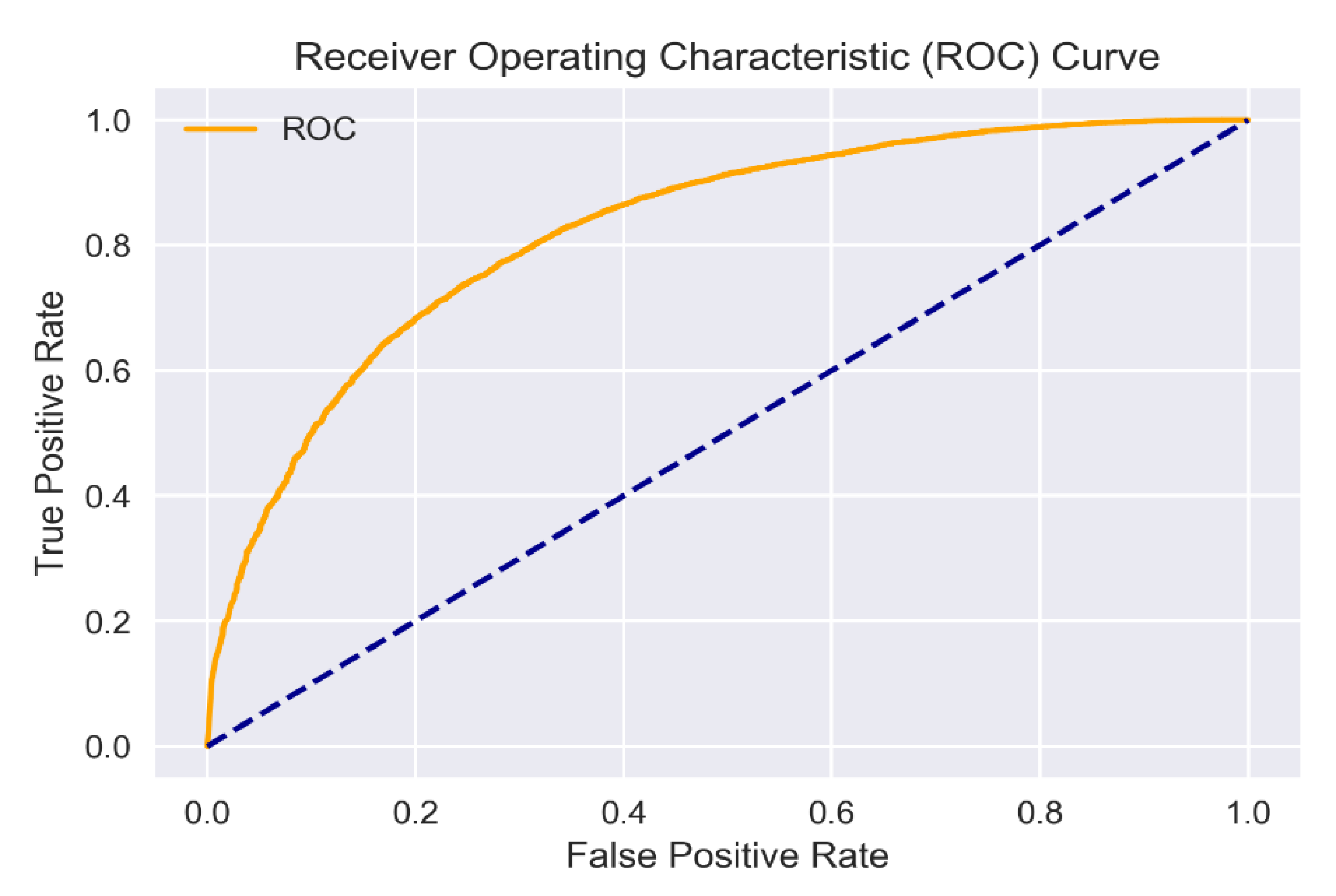
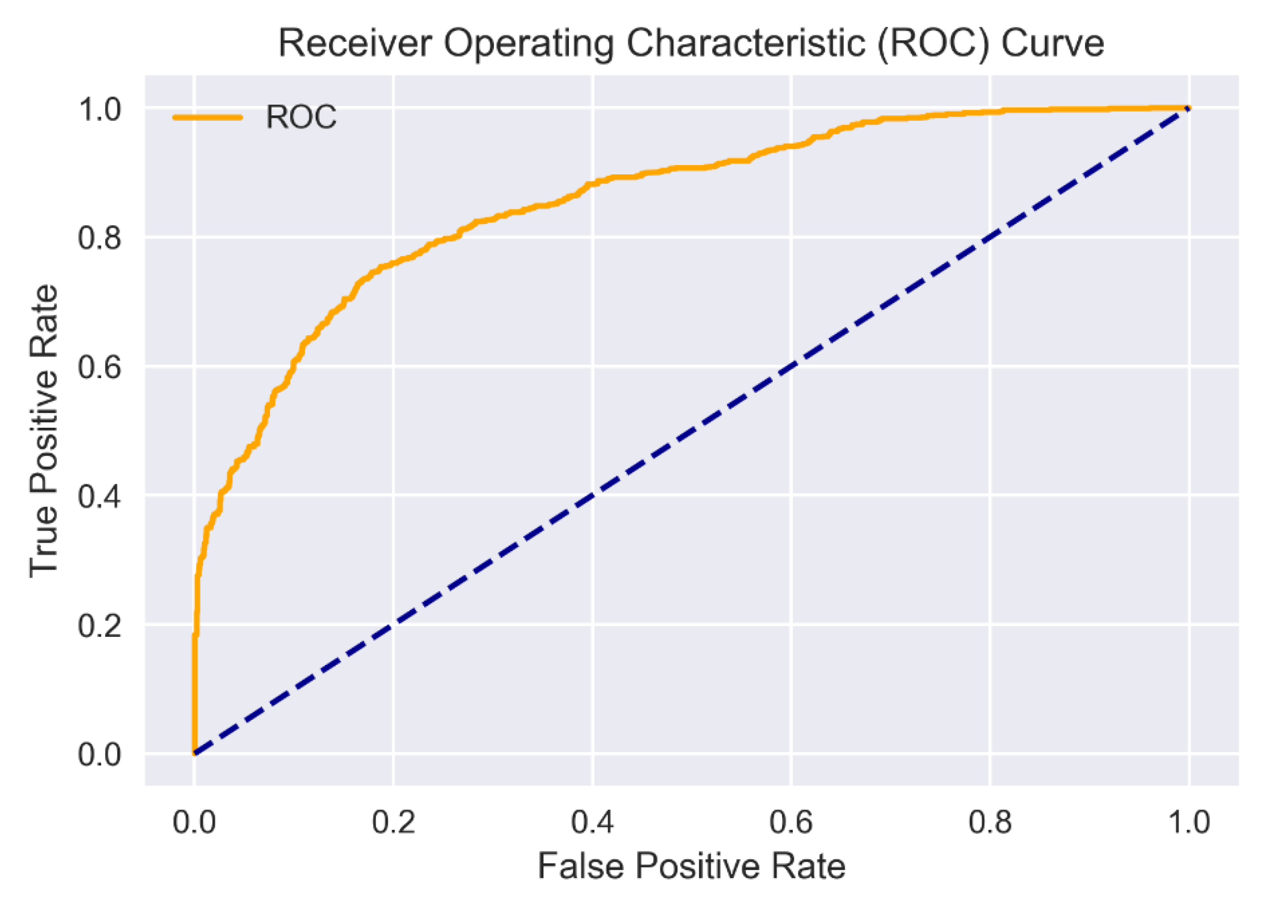
. Figure 2 and Figure 3 demonstrate the ROC curves of final classification results of LSTM + GloVe consolidation model for Turkish and English datasets, respectively. Deep learning methods are abbreviated as RNN: recurrent neural network, CNN: convolutional neural network, LSTM: long short-term memory network. In Table 4 and Table 5, among the results produced by each combination of deep learning models created using word embedding methods, the best ones are shown in bold letters. For both English and Turkish datasets, the combination of LSTM and GloVe generally offers the best classification results when the results of the experiment are evaluated.

For the Turkish dataset, an accuracy of 85.97% was obtained, while for the English dataset, an accuracy of 78.46% was achieved when cross validation results are considered. The combination of LSTM and GloVe was observed to be close to the other experiment results according to the results of the experiment produced by word embedding models and deep learning methods in terms of accuracy results. As seen in Table 4 and Table 5, the combination of LSTM and GloVe is a more suitable classification model for both languages on the sentiment analysis side. The dense structure of the LSTM model requires more computational power and time. Given the results and the duration of the experiment, although the combination of LSTM and GloVe is close to the others, as mentioned earlier, it is expected that the performance will increase further once sufficient computational capacity is achieved.

In order to perform the time series analysis, 249 days of data were collected from the exchange rate data which had to be obtained from the Central Bank of the Republic of Turkey for 365 days retrospectively, and 116 days of data were lost. It was observed that the optimal model for lost data was a quadratic decal calculation model, and the values were compared and verified with the Twitter exchange rate data shared on the relevant day.

Table 6. Experimental results obtained with time series analysis models.

Evaluation Metric	SES	HLT	HWC	HWT	ARIMA
MAPE	2.6432	2.4576	2.6325	2.6273	2.7144
MAE	0.0442	0.0412	0.0440	0.0439	0.0472
MSE	0.0024	0.0026	0.0024	0.0023	0.0020
Accuracy	95.58	95.87	95.59	95.60	92.99

presents the results of the experiments obtained by time series analysis methods. The abbreviations in the table are as follows: SES: simple exponential smoothing, HLT: Holt’s linear trend, HWC: Holt–Winters multiplicative, HWT: Holt–Winters additive, ARIMA: auto-regressive integrated moving average, MAPE: mean absolute percentage error, MAE: mean absolute error and MSE: mean squared error. Smoothing levels of 0.2, 0.4, 0.6, 0.8 were applied on each model. The results presented in the tables are at the smoothing level, where each model achieves the highest values. The most successful results on the SES and HLT models were at 0.8 smoothing levels, while the other models had the most performance results at 0.2 smoothing levels. It is clearly observed that the usage of the HLT model exhibits remarkable experiment results, with 95.87% accuracy, compared to the others.

Holt’s linear trend model was achieved by applying four different smoothing slopes to the exchange rate dataset, and the best one was chosen. Holt’s linear trend method consists of a trend component such as one level and one change in the trend. The level, i.e., the smoothing parameter, was considered as an alpha value. Three different levels are carried out as the smoothing parameter. At the same time, a slope value was used to predict the trend. In Holt’s linear implementation, alpha is a smoothing parameter between 0 and 1, while beta is the smoothing parameter used for the trend. When the results of the experiment were evaluated, it was observed that the worst prediction model with an accuracy of 71.11% was achieved with a smoothing value of 0.6. On the other hand, it is observed that the best rate estimate is achieved with an accuracy value of 95.87 when the smoothing parameter is set to 0.8 and the best tracking pattern for currency movements is achieved with a smoothing level of 0.8.

As a last step, the user can direct the investment by consolidating decisions of LSTM + GloVe and Holt’s linear trend model for both the Turkish and English datasets to get the final decision of the proposed system.

6. Discussion and Conclusions

Our goal is to produce a more consistent model by analyzing not only a method based on time series analysis, but also individuals on social media platforms such as Twitter that hold the pulse of society’s opinions about the direction of exchange rate. In this study, we propose a hybrid model that predicts the direction of US Dollar/Turkish Lira exchange rate by blending different approaches. For this purpose, deep learning-based financial sentiment analysis and time series analysis-based exchange rate prediction models are evaluated. Because there are many investors directing their investments according to comments made by experts on social media platforms, we concentrate on the sentiment analysis of people who share opinion on US Dollar/Turkish Lira exchange rate. For this purpose, financial sentiment analysis was carried out through Twitter, along with natural language processing techniques and word embedding methods applied to the data informing users of the daily economic developments and the exchange rate views that reflect this.

Daily exchange rates were collected within a certain date, and time series analysis methods were applied through the interface presented by the Central Bank of the Republic of Turkey and which is open to all. Turkish and English datasets collected from the Twitter social media platform were collected in the same date range as the numerical data in order to show consistency with time series analysis and to improve the performance of the model to be created. In order to obtain reliable results, methods such as parsing the source data, finding the correct states of words in the dictionary, finding the roots of words, normalization of words, clearing unused characters and words were applied to the dataset within the scope of pre-processing. Word vectors derived from word placement methods such as Word2Vec, GloVe, and fastText are given as the input to deep learning models such as LSTM, RNN, and CNN. During the training of each model, the dataset is divided into 80% training and 20% test datasets. The results of the experiment were examined and the model with the highest accuracy was selected. Turkish and English datasets with the highest performance of 86.03% and 79.01% regarding accuracy, respectively, were obtained from the combination of LSTM + GloVe. The advantage of both count-based statistics of word co-occurrences of GloVe model and long-short term dependencies of the LSTM model have a significant role in terms of classification success for text based in the sentiment analysis side.

In the side of time series analysis, the Central Bank of the Republic of Turkey shares official exchange rate data. They are collected to cover the period of one year, since the missing data for holidays and weekends are filled from reliable resources shared on Twitter. This ensures continuity and consistency of analysis over numerical data analysis. For time series analysis, simple exponential smoothing, Holt’s linear trend, Holt–Winters multiplicative, Holt–Winters additive and ARIMA models were applied and the best performance among them was selected. Regarding time series analysis when the results of the experiment were examined, it was observed that the best performance belonged to Holt’s linear trend method with 95.87% accuracy. Because it models the trend and level of a time series, Holt’s linear trend model provides competitive results compared to the other models in terms of predicting the exchange rate of US Dollar/Turkish Lira. Moreover, flexibility in the level and trend by smoothing with different weights and expecting less data also offer an advantage. Because the exchange rate of US Dollar/Turkish Lira does not require a seasonality for forecasting, Holt’s linear trend is more convenient for the proposed system. The fact that Twitter data, which hold the pulse of society and sometimes lead to events, are incorporated into the model by analyzing emotions, rather than making predictions in the determination of exchange rate direction, makes analysts and investors a more consistent investment tool.

As a further study, we aim to design the proposed hybrid model in such a way that it returns instantaneously, as well as create hybrid models separate from sentiment analysis and time series analysis and create a stronger exchange rate prediction model than the combination of emerging hybrid models.