Data Analysis of Beach Sands’ Chemical Analysis Using Multivariate Statistical Methods and Heavy Metal Distribution Maps: The Case of Moonlight Beach Sands, Kemer, Antalya, Turkey


Abstract
1. Introduction
2. Materials and Methods
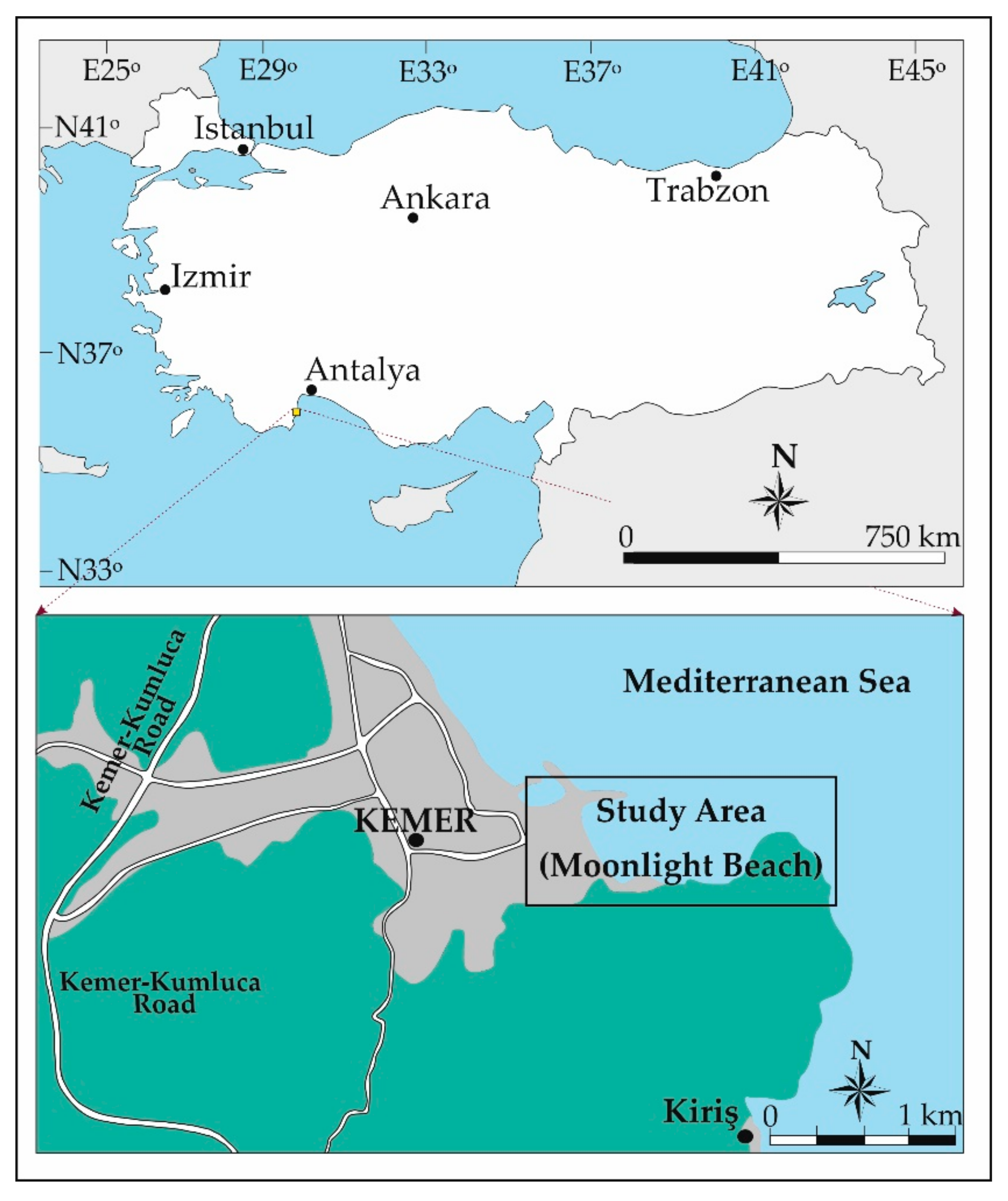
2.1. Study Site, Sampling, Experimental Analysis, Statistical Methods
2.2. Correlation Analysis
2.3. Factor Analysis
2.4. Regression Analysis
2.5. Calculation of Contamination Indices
3. Results and Discussion
3.1. Concentration and Descriptive Statistics in Sediment
3.2. Correlation Analysis
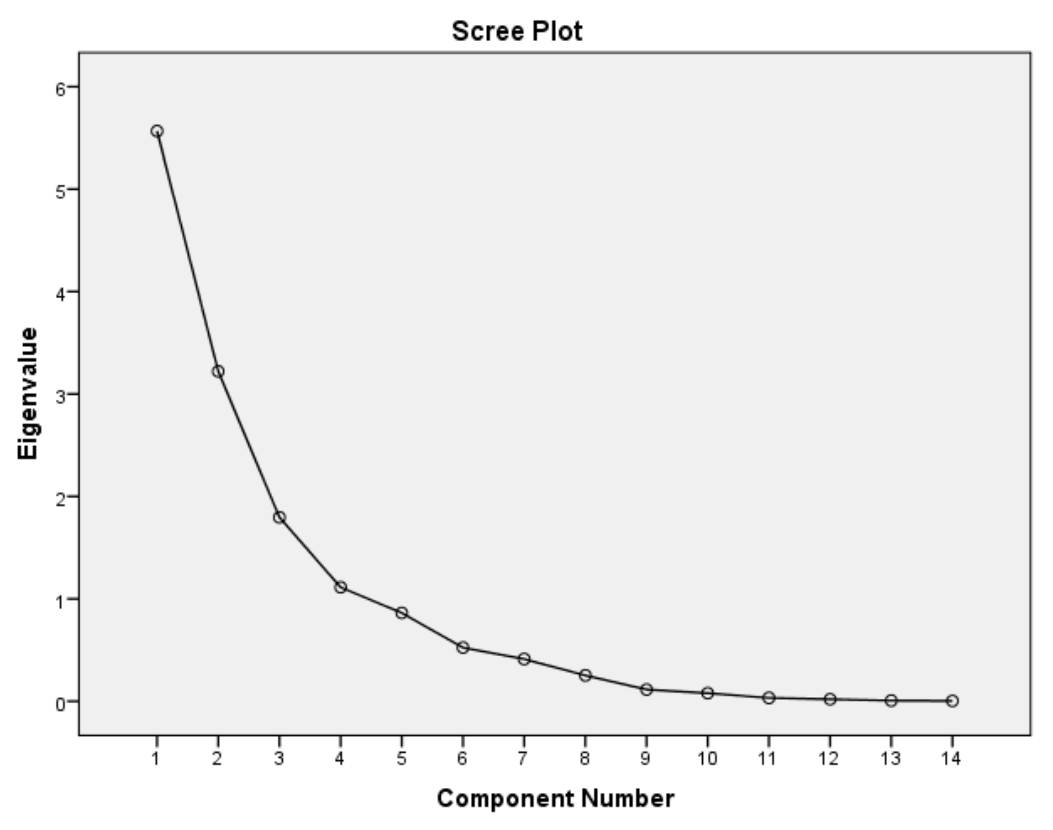
3.3. Factor Analysis
3.4. Regression Analysis
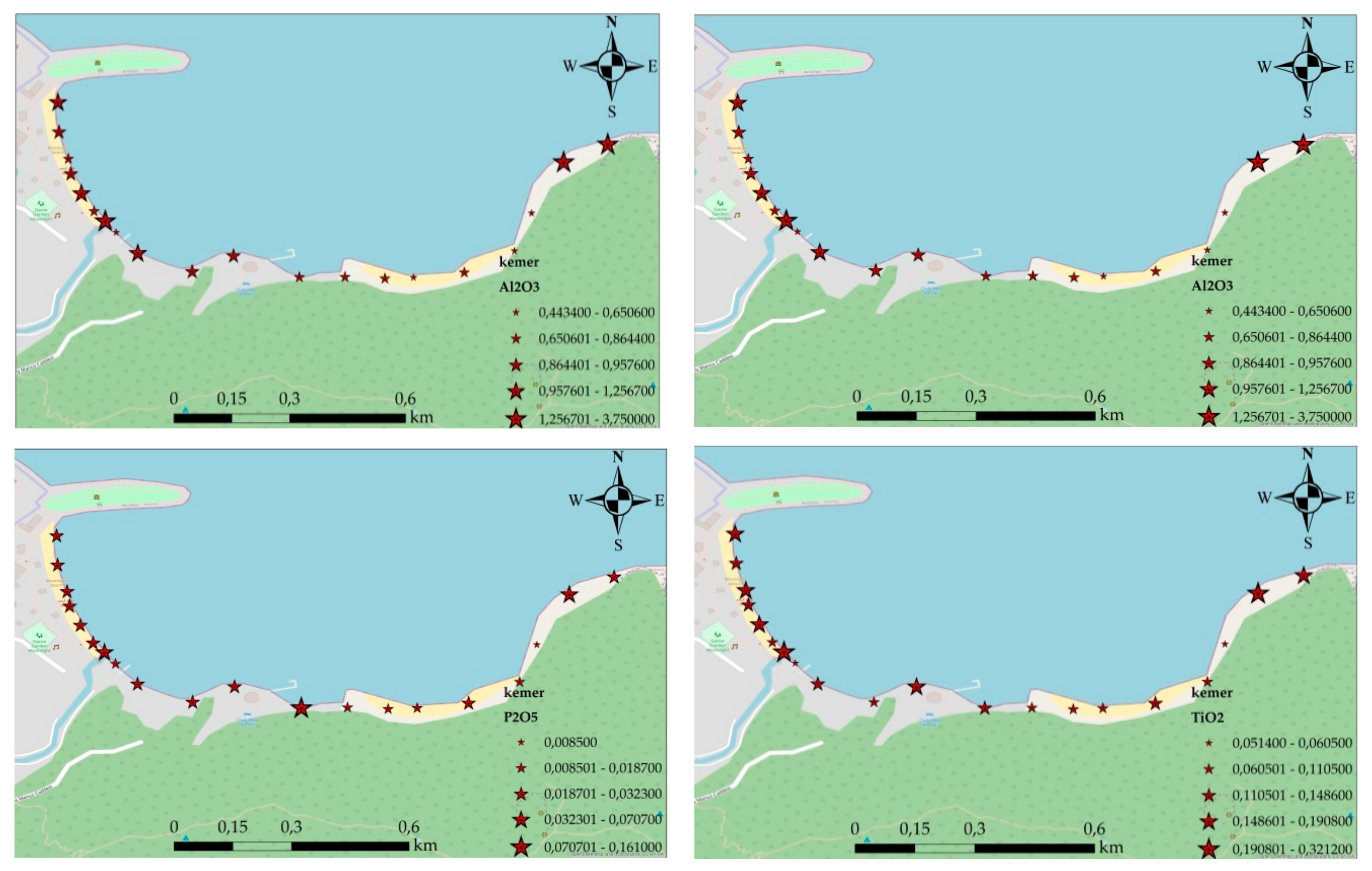
3.5. Metal Concentrations and Distribution in Baech
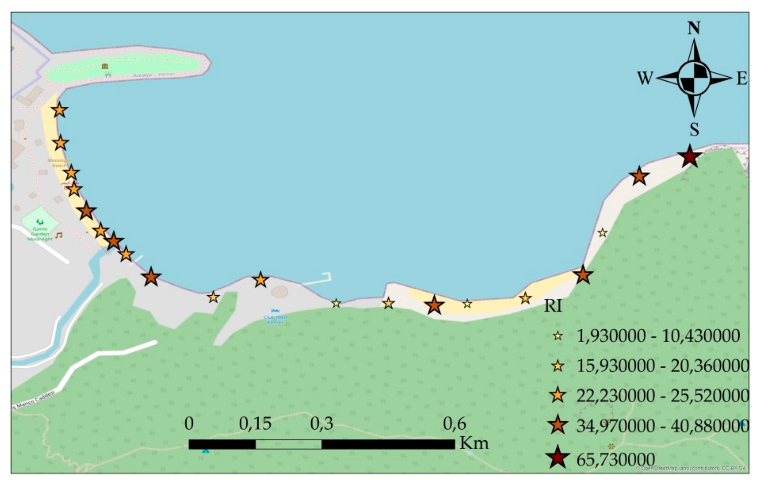
3.6. Results of Index
4. Conclusions
Funding
Acknowledgments
Conflicts of Interest
References
- Alshahri, F. Heavy metal contamination in sand and sediments near to disposal site of reject brine from desalination plant, Arabian Gulf: Assessment of environmental pollution. Environ. Sci. Pollut. Res. 2017, 24, 1821–1831. [Google Scholar] [CrossRef]
- Armstrong-Altrin, J.S.; Botello, A.V.; Villanueva, S.F.; Soto, L.A. Geochemistry of surface sediments from the northwestern Gulf of Mexico: Implications for provenance and heavy metal contamination. Geol. Q. 2019, 63, 522–538. [Google Scholar] [CrossRef]
- Barakat, A.; El Baghdadi, M.; Rais, J.; Nadem, S. Assessment of heavy metal in surface sediments of Day River at Beni-Mellal region, Morocco. Res. J. Environ. Earth Sci. 2012, 4, 797–806. [Google Scholar]
- Bramha, S.N.; Mohanty, A.K.; Satpathy, K.K.; Kanagasabapathy, K.V.; Panigrahi, S.; Samantara, M.K.; Prasad, M.V.R. Heavy metal content in the beach sediment with respect to contamination levels and sediment quality guidelines: A study at Kalpakkam coast, southeast coast of India. Environ. Earth Sci. 2014, 72, 4463–4472. [Google Scholar] [CrossRef]
- Bryant, F.B.; Yarnold, P.R. Principal-components analysis and exploratory and confirmatory factor analysis In Reading and Understanding Multivariate Statistics; Grimm, L.G., Yarnold, P.R., Eds.; American Psychological Association: Washington, DC, USA, 1995. [Google Scholar]
- Buzzi, N.S.; Marcovecchio, J.E. Heavy metal concentrations in sediments and in mussels from Argentinean coastal environments, South America. Environ. Earth Sci. 2018, 77, 321. [Google Scholar] [CrossRef]
- Carvalho, S.; Cunha, M.R.; Pereira, F.; Pousão-Ferreira, P.; Santos, M.N.; Gaspar, M.B. The effect of depth and sediment type on the spatial distribution of shallow soft-bottom amphipods along the southern Portuguese coast. Helgol. Mar. Res. 2012, 66, 489. [Google Scholar] [CrossRef]
- Chandramohan, J.; Chandrasekaran, A.; Jebakumar, J.P.P.; Elango, G.; Ravisankar, R. Assessment of Contamination by Metals in Coastal Sediments from South East Coast of Tamil Nadu, India with Statistical Approach. Iran. J. Sci. Technol. Trans. A Sci. 2018, 42, 1989–2004. [Google Scholar] [CrossRef]
- Chen, P.Y.; Popovich, P.M. Correlation: Parametric and Nonparametric Measures; Sage Publications: Thousand Oaks, CA, USA, 2002. [Google Scholar]
- Elias, M.S.; Ibrahim, S.; Samuding, K.; Ab Rahman, S.; Hashim, A. The sources and ecological risk assessment of elemental pollution in sediment of Linggi estuary, Malaysia. Mar. Pollut. Bull. 2018, 137, 646–655. [Google Scholar] [CrossRef]
- Francke, A.; Wennrich, V.; Sauerbrey, M.A.; Juschus, O.; Melles, M.; Brigham-Grette, J. Multivariate Statistic and Time Series Analyses of Grain-Size Data in Quaternary Sediments of Lake El’gygytgyn, NE Russia; University of Wollongong Australia: Wollongong, Australia, 2013. [Google Scholar]
- Fujita, M.; Ide, Y.; Sato, D.; Kench, P.S.; Kuwahara, Y.; Yokoki, H.; Kayanne, H. Heavy metal contamination of coastal lagoon sediments: Fongafale Islet, Funafuti Atoll, Tuvalu. Chemosphere 2014, 95, 628–634. [Google Scholar] [CrossRef]
- Gargouri, D.; Gzam, M.; Kharroubi, A.; Jedoui, Y. Use of sediment quality indicators for heavy metals contamination and ecological risk assessment in urbanized coastal zones. Environ. Earth Sci. 2018, 77, 381. [Google Scholar] [CrossRef]
- Gunst, R.F.; Mason, R.L. Regression Analysis and Its Application: A Data-Oriented Approach; CRC Press: New York, NY, USA, 1980. [Google Scholar]
- Hakanson, L. An ecological risk index for aquatic pollution control. A sedimentological approach. Water Res. 1980, 14, 975–1001. [Google Scholar] [CrossRef]
- Huang, F.; Xu, Y.; Tan, Z.; Wu, Z.; Xu, H.; Shen, L.; Hu, Z. Assessment of pollutions and identification of sources of heavy metals in sediments from west coast of Shenzhen, China. Environ. Sci. Pollut. Res. 2018, 25, 3647–3656. [Google Scholar] [CrossRef]
- Jha, D.K.; Ratnam, K.; Rajaguru, S.; Dharani, G.; Devi, M.P.; Kirubagaran, R. Evaluation of trace metals in seawater, sediments, and bivalves of Nellore, southeast coast of India, by using multivariate and ecological tool. Mar. Pollut. Bull. 2019, 146, 1–10. [Google Scholar] [CrossRef]
- Joksimović, D.; Perošević, A.; Castelli, A.; Pestorić, B.; Šuković, D.; Đurović, D. Assessment of heavy metal pollution in surface sediments of the Montenegrin coast: A 10-year review. J. Soils Sediments 2020, 20, 2598–2607. [Google Scholar] [CrossRef]
- Kang, T.; Oh, J.H.; Hong, J.S.; Kim, D. Response of intertidal meiofaunal communities to heavy metal contamination in laboratory microcosm experiments. J. Coast. Res. 2018, 85, 361–365. [Google Scholar] [CrossRef]
- Keshavarzi, A.; Kumar, V. Spatial distribution and potential ecological risk assessment of heavy metals in agricultural soils of Northeastern Iran. Geol. Ecol. Landsc. 2020, 4, 87–103. [Google Scholar] [CrossRef]
- Khan, R.; Rouf, M.A.; Das, S.; Tamim, U.; Naher, K.; Podder, J.; Hossain, S.M. Spatial and multi-layered assessment of heavy metals in the sand of Cox’s-Bazar beach of Bangladesh. Reg. Stud. Mar. Sci. 2017, 16, 171–180. [Google Scholar] [CrossRef]
- Kim, S.M.; Choi, Y. Mapping Heavy Metal Concentrations in Beach Sands Using GIS and Portable XRF Data. J. Mar. Sci. Eng. 2019, 7, 42. [Google Scholar] [CrossRef]
- Joe, H. Multivariate Models and Multivariate Dependence Concepts; Chapman and Hall/CRC: New York, NY, USA, 1997. [Google Scholar]
- Nelsen, R.B.A. Introduction to Copulas; Springer Science & Business Media: Berlin, Germany, 2007. [Google Scholar]
- Salvadori, G.; De Michele, C. On the use of copulas in hydrology: Theory and practice. J. Hydrol. Eng. 2007, 12, 369–380. [Google Scholar] [CrossRef]
- Salvadori, G.; Tomasicchio, G.R.; D’Alessandro, F. Practical guidelines for multivariate analysis and design in coastal and off-shore engineering. Coast. Eng. 2014, 88, 1–14. [Google Scholar] [CrossRef]
- Kline, P. A General Description of Factor Analysis. An Easy Guide to Factor Analysis; Taylor & Francis: Abingdon, UK, 1994. [Google Scholar]
- Lv, J.; Xia, Q.; Yan, T.; Zhang, M.; Wang, Z.; Zhu, L. Identifying the sources, spatial distributions, and pollution status of heavy metals in soils from the southern coast of Laizhou Bay, eastern China. Hum. Ecol. Risk Assess. Int. J. 2019, 25, 1953–1967. [Google Scholar] [CrossRef]
- Marinho, B.; Coelho, C.; Larson, M.; Hanson, H. Monitoring the evolution of nearshore nourishments along Barra-Vagueira coastal stretch, Portugal. Ocean Coast Manag. 2018, 157, 23–39. [Google Scholar] [CrossRef]
- Marrugo-Negrete, J.; Pinedo-Hernández, J.; Díez, S. Assessment of heavy metal pollution, spatial distribution and origin in agricultural soils along the Sinú River Basin, Colombia. Environ. Res. 2017, 154, 380–388. [Google Scholar] [CrossRef] [PubMed]
- Mohanty, B.; Nayak, A.; Dash, B.; Rout, S.S.; Kumar, B.C.; Patnaik, L.; Raut, D. Biodiversity and ecological considerations of brachyuran crabs (Crustacea: Decapoda) from Devi estuary–mangrove region on the east coast of India. Reg. Stud. Mar. Sci. 2019, 32, 100865. [Google Scholar] [CrossRef]
- Myrzabaeva, M.; Insepov, Z.; Boguspaev, K.K.; Faleev, D.G.; Nazhipkyzy, M.; Lesbayev, B.T.; Mansurov, Z.A. Investigation of nanohydrophobic sand as an insulating layer for cultivation of plants in soils contaminated with heavy metals. Eurasian Chem. Technol. J. 2017, 19, 91–98. [Google Scholar] [CrossRef]
- Nobi, E.P.; Dilipan, E.; Thangaradjou, T.; Sivakumar, K.; Kannan, L. Geochemical and geo-statistical assessment of heavy metal concentration in the sediments of different coastal ecosystems of Andaman Islands, India. Estuar. Coast. Shelf Sci. 2010, 87, 253–264. [Google Scholar] [CrossRef]
- Nour, H.E.; El-Sorogy, A.S.; Abdel-Wahab, M.; Almadani, S.; Alfaifi, H.; Youssef, M. Assessment of sediment quality using different pollution indicators and statistical analyses, Hurghada area, Red Sea coast, Egypt. Mar. Pollut. Bull. 2018, 133, 808–813. [Google Scholar] [CrossRef]
- Nour, H.E.S. Distribution, ecological risk, and source analysis of heavy metals in recent beach sediments of Sharm El-Sheikh, Egypt. Environ. Monit. Assess. 2019, 191, 546. [Google Scholar] [CrossRef]
- Rajkumar, H.; Naik, P.K.; Rishi, M.S. Evaluation of heavy metal contamination in soil using geochemical indexing approaches and chemometric techniques. Int. J. Environ. Sci. Technol. 2019, 16, 7467–7486. [Google Scholar] [CrossRef]
- Ramasamy, V.; Sundarrajan, M.; Suresh, G.; Paramasivam, K.; Meenakshisundaram, V. Role of light and heavy minerals on natural radioactivity level of high background radiation area, Kerala, India. Appl. Radiat. Isot. 2014, 85, 1–10. [Google Scholar] [CrossRef]
- Sahoo, P.K.; Dall’Agnol, R.; Salomão, G.N.; Junior, J.D.S.F.; da Silva, M.S.; Martins, G.C.; da Costa, M.F. Source and background threshold values of potentially toxic elements in soils by multivariate statistics and GIS-based mapping: A high density sampling survey in the Parauapebas basin, Brazilian Amazon. Environ. Geochem. Health 2020, 42, 255–282. [Google Scholar] [CrossRef] [PubMed]
- Sampaio, L.; Mamede, R.; Ricardo, F.; Magalhaes, L.; Rocha, H.; Martins, R.; Quintino, V. Soft-sediment crustacean diversity and distribution along the Portuguese continental shelf. J. Mar. Syst. 2016, 163, 43–60. [Google Scholar] [CrossRef]
- Sany, S.B.T.; Salleh, A.; Rezayi, M.; Saadati, N.; Narimany, L.; Tehrani, G.M. Distribution and contamination of heavy metal in the coastal sediments of Port Klang, Selangor, Malaysia. Water Air Soil Pollut. 2013, 224, 1476. [Google Scholar] [CrossRef]
- Satheeswaran, T.; Yuvaraj, P.; Damotharan, P.; Karthikeyan, V.; Jha, D.K.; Dharani, G.; Kirubagaran, R. Assessment of trace metal contamination in the marine sediment, seawater, and bivalves of Parangipettai, southeast coast of India. Mar. Pollut. Bull. 2019, 149, 110499. [Google Scholar] [CrossRef] [PubMed]
- Shabankareh, M.G.; Amanipoor, H.; Battaleb-Looie, S.; Khatooni, J.D. Statistical modeling the effect of sediment physicochemical properties on the concentration of heavy metal (case study: Musa Creek, SW Iran). Environ. Earth Sci. 2018, 77, 101. [Google Scholar] [CrossRef]
- Shakir, E.; Al Mashhady, A.A.; Al-Janabi, Z.Z.; Al-Obaidy, A.H.M. Geochemical and geo-statistical assessment of heavy metals concentration in sediment of Shatt Al-Basrah, Iraq. J. Basic Appl. Res. Int. 2016, 233–239. [Google Scholar]
- Suresh, G.; Ramasamy, V.; Sundarrajan, M.; Paramasivam, K. Spatial and vertical distributions of heavy metals and their potential toxicity levels in various beach sediments from high-background-radiation area, Kerala, India. Mar. Pollut. Bull. 2015, 91, 389–400. [Google Scholar] [CrossRef]
- Stamatis, N.; Kamidis, N.; Pigada, P.; Sylaios, G.; Koutrakis, E. Quality indicators and possible ecological risks of heavy metals in the sediments of three semi-closed East Mediterranean Gulfs. Toxics 2019, 7, 30. [Google Scholar] [CrossRef]
- Tomlinson, D.L.; Wilson, J.G.; Harris, C.R.; Jeffrey, D.W. Problems in the assessment of heavy-metal levels in estuaries and the formation of a pollution index. Helgoländer Meeresunters. 1980, 33, 566–575. [Google Scholar] [CrossRef]
- Ugolini, A.; Borghini, F.; Focardi, S.; Chelazzi, G. Heavy metals accumulation in two syntopic sandhopper species: Talitrus saltator (Montagu) and Talorchestia ugolinii Bellan Santini and Ruffo. Mar. Pollut. Bull. 2005, 50, 1328–1334. [Google Scholar] [CrossRef]
- Ustaoglu, F.; Tepe, Y.; Aydin, H. Heavy metals in sediments of two nearby streams from Southeastern Black Sea coast: Contamination and ecological risk assessment. Environ. Forensics 2020, 21, 145–156. [Google Scholar] [CrossRef]
- Veerasingam, S.; Venkatachalapathy, R.; Ramkumar, T. Distribution of clay minerals in marine sediments off Chennai, Bay of Bengal, India: Indicators of sediment sources and transport processes. Int. J. Sediment. Res. 2014, 29, 11–23. [Google Scholar] [CrossRef]
- Vieira, L.R.; Morgado, F.; Nogueira, A.J.; Soares, A.M.; Guilhermino, L. Integrated multivariate approach of ecological and ecotoxicological parameters in coastal environmental monitoring studies. Ecol. Indic. 2018, 95, 1128–1142. [Google Scholar] [CrossRef]
- Williams, J.A.; Antoine, J. Evaluation of the elemental pollution status of Jamaican surface sediments using enrichment factor, geoaccumulation index, ecological risk and potential ecological risk index. Mar. Pollut. Bull. 2020, 157, 111288. [Google Scholar] [CrossRef] [PubMed]
- Yalcin, M.G.; Ilhan, S. Multivariate analyses to determine the origin of potentially harmful heavy metals in beach and dune sediments from Kizkalesi coast (Mersin), Turkey. Bull. Environ. Contam. Toxicol. 2008, 81, 57–68. [Google Scholar] [CrossRef]
- Yalcin, M.G. Heavy mineral distribution as related to environmental conditions for modern beach sediments from the Susanoglu (Atakent, Mersin, Turkey). Environ. Geol. 2009, 58, 119–129. [Google Scholar] [CrossRef]
- Yalcin, M.G.; Setti, M.; Karakaya, F.; Sacchi, E.; Ilbeyli, N. Geochemical and mineralogical characteristics of beach sediments along the coast between Alanya and Silifke (Southern Turkey). Clay Miner. 2015, 50, 233–248. [Google Scholar] [CrossRef]
- Yalcin, F.; Nyamsari, D.G.; Paksu, E.; Yalcin, M.G. Statistical Assessment of Heavy Metal Distribution and Contamination of Beach Sands of Antalya-Turkey: An Approach to the Multivariate Analysis Techniques. Filomat 2016, 30, 945–952. [Google Scholar] [CrossRef]
- Yalcin, M.G.; Simsek, G.; Ocak, S.B.; Yalcin, F.; Kalayci, Y.; Karaman, M.E. Multivariate statistics and heavy metals contamination in beach sediments from The Sakarya Canyon, Turkey. Asian J. Chem. 2013, 25, 2059–2066. [Google Scholar] [CrossRef]
- Yalcin, M.G.; Cevik, O.; Karaman, M.E. Use of multivariate statistics methods to determine grain size, heavy metal distribution and origins of heavy metals in Mersin Bay (Eastern Mediterranean) coastal sediments. Asian J. Chem. 2013, 25, 5. [Google Scholar] [CrossRef]
- Yalcin, M.G.; Coskun, B.; Nyamsari, D.G.; Yalcin, F. Geomedical, ecological risk, and statistical assessment of hazardous elements in shore sediments of the Iskenderun Gulf, Eastern Mediterranean, Turkey. Environ. Earth Sci. 2019, 78, 438. [Google Scholar] [CrossRef]
- Zhang, Y.; Hu, X.; Yu, T. Distribution and risk assessment of metals in sediments from Taihu Lake, China using multivariate statistics and multiple tools. Bull. Environ. Contam. Toxicol. 2012, 89, 1009–1015. [Google Scholar] [CrossRef]
- Yalcin, F.; Kilic, S.; Nyamsari, D.G.; Yalcin, M.G.; Kilic, M. Principal Component Analysis of Integ rated Metal Concentrations of Bogacayi Riverbank Sediments in Turkey. Pol. J. Environ. Stud. 2016, 25, 471–485. [Google Scholar] [CrossRef]
- Official Newspaper, Soil Pollution Control Regulation, 31 May 2005 and Numbered 25831. Available online: https://www.resmigazete.gov.tr/eskiler/2005/05/20050531.htm. (accessed on 17 September 2020).
- Yalcin, F.; Ilbeyli, N.; Demirbilek, M.; Yalcin, M.G.; Gunes, A.; Kaygusuz, A.; Ozmen, S.F. Estimation of natural radionuclides’ concentration of the plutonic rocks in the Sakarya Zone, Turkey using multivariate statistical methods. Symmetry 2020, 12, 1048. [Google Scholar] [CrossRef]
- Yalcin, F.; Unal, S.; Yalcin, M.G.; Akturk, O.; Ocak, S.B.; Ozmen, S.F. Investigation of the effect of hydrothermal waters on radionuclide activity concentrations in natural marble with multivariate statistical analysis. Symmetry 2020, 12, 1219. [Google Scholar] [CrossRef]


| Indices | Equation | Description | Reference |
|---|---|---|---|
| Contamination Factor (CF) | : Low contamination : Moderate contamination : High contamination : Very high contamination | [48,49] | |
| Pollution load index (PLI) | : No polluted : Only baseline levels of pollutans are present : Polluted | [50,51] | |
| Enrichment Factor (EF) | : No enrichment : Minor enrichment : Moderate enrichment : Moderately enrichment : High enrichment : Very high enrichment : Exceptionally high enrichment | [52,53] | |
| Potential Ecological Risk Index (RI) | : Low ecological risk : Moderate ecological risk Ecological risk : Very high ecological risk | [49] |
| Coordinate | Elements (%) | ||||||||||||||||||||||
|---|---|---|---|---|---|---|---|---|---|---|---|---|---|---|---|---|---|---|---|---|---|---|---|
| Sample Location | Latitude | Longitude | Ca | Si | Mg | Fe | Cl | Al | Na | S | K | Ti | Mn | Cr | Ni | P | Sr | Br | Zr | Rb | Ba | Zn | Cu |
| K1 | 36.598623 | 30.58785532 | 24.945 | 3.472 | 2.422 | 2.309 | 3.054 | 1.183 | 1.129 | 0.142 | 0.205 | 0.114 | 0.060 | 0.039 | 0.024 | 0.009 | 0.017 | 0.014 | 0.005 | 0 | 0 | 0 | 0 |
| K2 | 36.598224 | 30.58682825 | 29.023 | 5.104 | 2.908 | 1.931 | 0.054 | 1.375 | 0.206 | 0.040 | 0.273 | 0.183 | 0.057 | 0.017 | 0.013 | 0.029 | 0.030 | 0 | 0.006 | 0 | 0 | 0.004 | 0 |
| K3 | 36.597064 | 30.58608198 | 34.298 | 0.750 | 2.388 | 0.527 | 0.286 | 0.235 | 0.267 | 0.041 | 0.039 | 0.031 | 0.017 | 0 | 0 | 0.004 | 0.028 | 0 | 0 | 0 | 0 | 0 | 0 |
| K4 | 36.596218 | 30.58568363 | 34.094 | 1.786 | 2.041 | 0.837 | 0.615 | 0.344 | 0.519 | 0.067 | 0.084 | 0.054 | 0.029 | 0.010 | 0.017 | 0.007 | 0.045 | 0 | 0 | 0 | 0.036 | 0 | 0 |
| K5 | 36.595734 | 30.58451393 | 33.827 | 3.071 | 2.070 | 0.979 | 0.482 | 0.431 | 0.423 | 0.053 | 0.115 | 0.073 | 0.025 | 0.023 | 0 | 0.009 | 0.032 | 0.003 | 0 | 0 | 0 | 0 | 0 |
| K6 | 36.59562 | 30.58333271 | 34.479 | 2.059 | 1.950 | 0.663 | 0.245 | 0.310 | 0.218 | 0.042 | 0.074 | 0.056 | 0.023 | 0.008 | 0 | 0.005 | 0.038 | 0 | 0 | 0 | 0 | 0 | 0 |
| K7 | 36.595598 | 30.58266279 | 33.149 | 3.255 | 1.961 | 0.884 | 0.938 | 0.457 | 0.771 | 0.082 | 0.123 | 0.059 | 0.033 | 0.025 | 0.014 | 0.008 | 0.047 | 0.004 | 0 | 0 | 0 | 0 | 0 |
| K8 | 36.595633 | 30.581734 | 34.440 | 3.334 | 2.151 | 0.883 | 0.514 | 0.413 | 0.441 | 0.052 | 0.100 | 0.066 | 0.033 | 0.029 | 0 | 0.007 | 0.034 | 0 | 0 | 0 | 0 | 0 | 0 |
| K9 | 36.595629 | 30.58067228 | 28.498 | 1.996 | 1.705 | 0.936 | 0.411 | 0.391 | 0.376 | 0.049 | 0.084 | 0.071 | 0.027 | 0.013 | 0 | 0.070 | 0.034 | 0 | 0 | 0 | 0.037 | 0 | 0 |
| K10 | 36.596112 | 30.57913712 | 34.953 | 4.403 | 1.687 | 1.054 | 0.088 | 0.499 | 0.156 | 0.043 | 0.131 | 0.095 | 0.040 | 0.030 | 0 | 0.011 | 0.058 | 0 | 0 | 0 | 0 | 0.003 | 0 |
| K11 | 36.595759 | 30.57817575 | 33.919 | 4.777 | 1.919 | 0.989 | 0.266 | 0.507 | 0.343 | 0.054 | 0.114 | 0.065 | 0.012 | 0.025 | 0 | 0.010 | 0.055 | 0 | 0 | 0 | 0 | 0.005 | 0 |
| K12 | 36.596175 | 30.5769109 | 33.272 | 4.734 | 1.891 | 1.148 | 0.526 | 0.598 | 0.539 | 0.065 | 0.127 | 0.076 | 0.026 | 0.020 | 0.017 | 0.012 | 0.042 | 0 | 0 | 0 | 0.038 | 0 | 0 |
| K13 | 36.596633 | 30.57640476 | 34.059 | 2.556 | 2.282 | 0.644 | 0.454 | 0.324 | 0.426 | 0.051 | 0.075 | 0.036 | 0.012 | 0.020 | 0.007 | 0.006 | 0.031 | 0 | 0.005 | 0.003 | 0.000 | 0 | 0 |
| K14 | 36.596898 | 30.57615056 | 32.727 | 5.574 | 0.509 | 1.266 | 0 | 1.985 | 0.031 | 0.010 | 0.283 | 0.193 | 0.021 | 0.019 | 0.013 | 0.031 | 0.020 | 0 | 0 | 0.003 | 0.037 | 0.005 | 0 |
| K15 | 36.597109 | 30.57588688 | 30.329 | 3.784 | 2.086 | 0.730 | 0.361 | 0.457 | 0.382 | 0.044 | 0.107 | 0.061 | 0.019 | 0.022 | 0.006 | 0.009 | 0.028 | 0 | 0 | 0 | 0.037 | 0.003 | 0 |
| K16 | 36.597518 | 30.57559466 | 29.190 | 5.267 | 1.547 | 1.019 | 0.187 | 0.565 | 0.246 | 0.048 | 0.149 | 0.099 | 0.038 | 0.024 | 0.010 | 0.011 | 0.038 | 0 | 0 | 0.002 | 0.047 | 0.003 | 0 |
| K17 | 36.597955 | 30.57534626 | 33.679 | 3.554 | 2.179 | 0.872 | 0.351 | 0.507 | 0.348 | 0.060 | 0.108 | 0.076 | 0.030 | 0.019 | 0.007 | 0.010 | 0.048 | 0 | 0 | 0.002 | 0 | 0 | 0.010 |
| K18 | 36.598287 | 30.57529115 | 35.585 | 2.590 | 1.678 | 1.101 | 0.076 | 0.439 | 0.120 | 0.041 | 0.102 | 0.108 | 0.034 | 0.026 | 0 | 0.010 | 0.061 | 0 | 0 | 0 | 0.045 | 0.006 | 0 |
| K19 | 36.598895 | 30.5750709 | 34.509 | 2.792 | 1.995 | 1.054 | 0.141 | 0.477 | 0.184 | 0.051 | 0.115 | 0.089 | 0.055 | 0.028 | 0 | 0.013 | 0.051 | 0 | 0 | 0 | 0 | 0 | 0 |
| K20 | 36.599562 | 30.57505003 | 30.882 | 4.793 | 1.719 | 1.366 | 0.337 | 0.665 | 0.348 | 0.059 | 0.175 | 0.109 | 0.059 | 0.030 | 0 | 0.014 | 0.049 | 0 | 0 | 0 | 0.038 | 0.002 | 0 |
| Maxsimum | 35.585 | 5.574 | 2.908 | 2.309 | 3.054 | 1.985 | 1.129 | 0.142 | 0.283 | 0.193 | 0.060 | 0.039 | 0.024 | 0.070 | 0.061 | 0.014 | 0.006 | 0.003 | 0.047 | 0.006 | 0.010 | ||
| Minimum | 24.945 | 0.750 | 0.509 | 0.527 | 0 | 0.235 | 0.031 | 0.010 | 0.039 | 0.031 | 0.012 | 0 | 0 | 0.004 | 0.017 | 0 | 0 | 0 | 0 | 0 | 0 | ||
| Mean | 32.493 | 3.483 | 1.954 | 1.060 | 0.469 | 0.608 | 0.374 | 0.055 | 0.129 | 0.086 | 0.032 | 0.021 | 0.006 | 0.014 | 0.039 | 0.001 | 0.001 | 0 | 0.016 | 0.002 | 0 | ||
| Median | 33.753 | 3.403 | 1.978 | 0.984 | 0.344 | 0.467 | 0.348 | 0.051 | 0.115 | 0.074 | 0.029 | 0.023 | 0.003 | 0.010 | 0.038 | 0 | 0 | 0 | 0 | 0 | 0 | ||
| Standard Deviation | 2.764 | 1.319 | 0.463 | 0.421 | 0.648 | 0.425 | 0.244 | 0.025 | 0.062 | 0.042 | 0.015 | 0.009 | 0.008 | 0.015 | 0.012 | 0.003 | 0.002 | 0.001 | 0.020 | 0.002 | 0.002 | ||
| Kurtosis | 1.412 | −0.678 | 4.828 | 3.784 | 14.827 | 5.491 | 4.067 | 8.392 | 1.803 | 2.173 | −0.438 | 0.801 | −0.470 | 11.178 | −0.763 | 13.629 | 3.038 | 2.341 | −1.858 | −0.461 | 20.000 | ||
| Skewness | −1.375 | −0.181 | −1.204 | 1.805 | 3.652 | 2.348 | 1.671 | 2.248 | 1.406 | 1.444 | 0.704 | −0.583 | 0.830 | 3.179 | 0.053 | 3.585 | 2.160 | 1.914 | 0.499 | 0.976 | 4.472 | ||
| Kolmogorov-Smirnov | Shapiro-Wilk | |||
|---|---|---|---|---|
| Statistic | Sig. | Statistic | Sig. | |
| Ca | 0.244 | 0.003 | 0.834 | 0.003 |
| Si | 0.129 | 0.200 * | 0.969 | 0.724 ** |
| Mg | 0.176 | 0.108 * | 0.881 | 0.018 |
| Fe | 0.216 | 0.015 | 0.824 | 0.002 |
| Al | 0.310 | 0.000 | 0.678 | 0.000 |
| Na | 0.191 | 0.054 * | 0.867 | 0.011 |
| S | 0.224 | 0.010 | 0.752 | 0.000 |
| K | 0.239 | 0.004 | 0.850 | 0.005 |
| Ti | 0.187 | 0.064 * | 0.858 | 0.007 |
| Mn | 0.172 | 0.122 * | 0.906 | 0.054 * |
| Cr | 0.145 | 0.200 * | 0.966 | 0.677 * |
| Ni | 0.299 | 0.000 | 0.810 | 0.001 |
| P | 0.355 | 0.000 | 0.575 | 0.000 |
| Sr | 0.102 | 0.200 * | 0.975 | 0.857 * |
| Zr | 0.508 | 0.000 | 0.448 | 0.000 |
| Rb | 0.480 | 0.000 | 0.533 | 0.000 |
| Ba | 0.385 | 0.000 | 0.683 | 0.000 |
| Zn | 0.367 | 0.000 | 0.739 | 0.000 |
| Cu | 0.538 | 0.000 | 0.236 | 0.000 |
| Ca | Si | Mg | Fe | Al | Na | S | K | Ti | Mn | Cr | Ni | P | Sr | Zr | Rb | Ba | Zn | Cu | |
|---|---|---|---|---|---|---|---|---|---|---|---|---|---|---|---|---|---|---|---|
| Ca | 1.000 | ||||||||||||||||||
| Si | −0.445 * | 1.000 | |||||||||||||||||
| Mg | −0.101 | −0.295 | 1.000 | ||||||||||||||||
| Fe | −0.347 | 0.647 ** | −0.302 | 1.000 | |||||||||||||||
| Al | −0.529 * | 0.888 ** | −0.194 | 0.842 ** | 1.000 | ||||||||||||||
| Na | −0.337 | −0.226 | 0.432 | −0.203 | −0.159 | 1.000 | |||||||||||||
| S | −0.203 | −0.077 | 0.232 | 0.005 | 0.069 | 0.827 ** | 1.000 | ||||||||||||
| K | −0.481 * | 0.838 ** | −0.229 | 0.865 ** | 0.938 ** | −0.140 | 0.060 | 1.000 | |||||||||||
| Ti | −0.344 | 0.690 ** | −0.323 | 0.925 ** | 0.849 ** | −0.392 | −0.192 | 0.844 ** | 1.000 | ||||||||||
| Mn | −0.160 | 0.267 | −0.028 | 0.658 ** | 0.483 * | −0.057 | 0.157 | 0.566 ** | 0.663 ** | 1.000 | |||||||||
| Cr | 0.071 | 0.361 | −0.168 | 0.516 * | 0.384 | 0.071 | 0.289 | 0.468* | 0.441 | 0.553 * | 1.000 | ||||||||
| Ni | −0.522 * | 0.270 | 0.209 | 0.240 | 0.432 | 0.457 * | 0.380 | 0.422 | 0.168 | 0.128 | −0.133 | 1.000 | |||||||
| P | −0.435 | 0.596 ** | −0.482 * | 0.710 ** | 0.705 ** | −0.396 | −0.203 | 0.642 ** | 0.762 ** | 0.403 | 0.149 | 0.052 | 1.000 | ||||||
| Sr | 0.540 * | −0.026 | −0.466 * | 0.096 | −0.029 | −0.257 | 0.170 | −0.048 | 0.021 | 0.242 | 0.320 | −0.377 | 0.151 | 1.000 | |||||
| Zr | −0.375 | 0.092 | 0.600 ** | 0.271 | 0.244 | 0.181 | 0.015 | 0.244 | 0.223 | 0.234 | 0.051 | 0.460 * | −0.024 | −0.474 * | 1.000 | ||||
| Rb | −0.172 | 0.312 | −0.161 | −0.083 | 0.222 | −0.214 | −0.174 | 0.151 | 0.144 | −0.238 | −0.172 | 0.285 | 0.140 | −0.240 | 0.119 | 1.000 | |||
| Ba | −0.265 | 0.305 | −0.660 ** | 0.304 | 0.271 | −0.138 | −0.151 | 0.212 | 0.356 | 0.082 | −0.006 | 0.148 | 0.467 * | 0.084 | −0.328 | 0.188 | 1.000 | ||
| Zn | −0.033 | 0.619 ** | −0.480 * | 0.475 * | 0.487 * | −0.651 ** | −0.549 * | 0.447 * | 0.536 * | 0.083 | 0.240 | −0.113 | 0.452 * | 0.194 | −0.012 | 0.143 | 0.408 | 1.000 | |
| Cu | −0.020 | 0.060 | 0.219 | −0.179 | 0.139 | −0.020 | 0.219 | −0.060 | 0.020 | 0.020 | −0.179 | 0.064 | 0.060 | 0.179 | −0.096 | 0.370 | −0.180 | −0.180 | 1.000 |
| Kaiser-Meyer-Olkin Measure of Sampling Adequacy | 0.529 | |
| Bartlett’s Test of Sphericity | Approx. Chi-Square | 301.027 |
| Sig. | 0.000 | |
| Initial | Extraction | |
|---|---|---|
| Ca | 1.000 | 0.826 |
| Si | 1.000 | 0.770 |
| Mg | 1.000 | 0.540 |
| Fe | 1.000 | 0.931 |
| Al | 1.000 | 0.943 |
| Na | 1.000 | 0.907 |
| S | 1.000 | 0.936 |
| K | 1.000 | 0.965 |
| Ti | 1.000 | 0.943 |
| Mn | 1.000 | 0.830 |
| Cr | 1.000 | 0.767 |
| Ni | 1.000 | 0.800 |
| P | 1.000 | 0.752 |
| Sr | 1.000 | 0.786 |
| Component | Initial Eigenvalues | Extraction Sums of Squared Loadings | Rotation Sums of Squared Loadings | ||||||
|---|---|---|---|---|---|---|---|---|---|
| Total | % of Variance | Cumulative % | Total | % of Variance | Cumulative % | Total | % of Variance | Cumulative % | |
| 1 | 5.567 | 39.766 | 39.766 | 5.567 | 39.766 | 39.766 | 4.282 | 30.584 | 30.584 |
| 2 | 3.220 | 23.002 | 62.769 | 3.220 | 23.002 | 62.769 | 3.421 | 24.434 | 55.018 |
| 3 | 1.795 | 12.825 | 75.593 | 1.795 | 12.825 | 75.593 | 2.271 | 16.223 | 71.242 |
| 4 | 1.112 | 7.946 | 83.540 | 1.112 | 7.946 | 83.540 | 1.722 | 12.298 | 83.540 |
| Component | ||||
|---|---|---|---|---|
| 1 | 2 | 3 | 4 | |
| Al | 0.921 | 0.158 | −0.006 | 0.265 |
| K | 0.912 | 0.143 | 0.232 | 0.242 |
| Ti | 0.870 | −0.089 | 0.258 | 0.334 |
| Si | 0.818 | −0.082 | 0.278 | −0.131 |
| Mg | −0.512 | 0.460 | 0.224 | 0.121 |
| Na | −0.172 | 0.912 | 0.168 | −0.135 |
| S | −0.178 | 0.847 | 0.413 | −0.128 |
| Ni | 0.458 | 0.761 | −0.090 | −0.055 |
| Ca | −0.278 | −0.616 | −0.220 | −0.567 |
| Sr | −0.274 | −0.561 | 0.490 | −0.395 |
| Mn | 0.222 | 0.209 | 0.820 | 0.254 |
| Cr | 0.328 | 0.174 | 0.736 | −0.295 |
| Fe | 0.555 | 0.474 | 0.559 | 0.294 |
| P | 0.157 | −0.172 | −0.035 | 0.835 |
| Model Summary | R | R Square | Adjusted R Square | Std. Error of the Estimate | Change Statistics | Durbin-Watson | ||||||
| R Square Change | F Change | df1 | df2 | Sig. F Change | ||||||||
| 0.798 a | 0.636 | 0.468 | 0.961617579534837 | 0.636 | 3.790 | 6 | 13 | 0.021 | 1.597 | |||
| Model ANOVA | Sum of Squares | df | Mean Square | F | Sig. | |||||||
| Regression | 21.030 | 6 | 3.505 | 3.790 | 0.021 b | |||||||
| Residual | 12.021 | 13 | 0.925 | |||||||||
| Total | 33.051 | 19 | ||||||||||
| Coefficients a Model | Unstandardized Coefficients | Standardized Coefficients | t | Sig. | Correlations | Collinearity Statistics | ||||||
| B | Std. Error | Beta | Zero-order | Partial | Part | Tolerance | VIF | |||||
| (Constant) | 0.419 | 1.920 | 0.218 | 0.831 | ||||||||
| Mg | 0.073 | 0.619 | 0.026 | 0.118 | 0.908 | −0.340 | 0.033 | 0.020 | 0.592 | 1.689 | ||
| Na | 0.002 | 1.374 | 0 | 0.002 | 0.999 | −0.137 | 0 | 0 | 0.432 | 2.314 | ||
| Ti | 23.495 | 9.021 | 0.744 | 2.605 | 0.022 | 0.671 | 0.586 | 0.436 | 0.343 | 2.916 | ||
| Mn | −32.358 | 23.717 | −0.369 | −1.364 | 0.196 | 0.275 | −0.354 | −0.228 | 0.382 | 2.619 | ||
| Cr | 70.171 | 35.435 | 0.473 | 1.980 | 0.069 | 0.518 | 0.481 | 0.331 | 0.490 | 2.040 | ||
| Sr | 11.617 | 24.093 | 0.108 | 0.482 | 0.638 | 0.020 | 0.133 | 0.081 | 0.561 | 1.784 | ||
| Turkey’s MPC | Contamination Factor | Enrichment Factor | Potential Ecological Risk index | Risk | |||||||||
|---|---|---|---|---|---|---|---|---|---|---|---|---|---|
| Mean | Min | Max | Mean | Min | Max | Mean | Min | Max | Mean | Min | Max | ||
| Mn | - | - | - | - | 5.03 | 1.63 | 6.40 | 3.61 | 1.32 | 6.68 | |||
| Cr | 100 | 2.139 | 0 | 3.866 | 4.74 | 0 | 6.40 | 12.22 | 0 | 22.09 | |||
| Ni | 30-75 | 0.844 | 0 | 3.154 | 2.22 | 0 | 6.20 | 9.90 | 0 | 36.96 | |||
| Cu | 50–140 | 0.035 | 0 | 0.690 | 0.22 | 0 | 4.39 | - | - | - | |||
| Zn | 150–300 | 0.028 | 0 | 0.207 | 1.79 | 0 | 6.40 | 0.94 | 0 | 3.82 | |||
| RI | 26.67 | 1.93 | 65.73 | ||||||||||
| Sample | RI | PLI | Cr (CF) | Cr (EF) |
|---|---|---|---|---|
| K1 | 65.73 | 1.213 | 3.86573 | 4.98 |
| K2 | 39.69 | 0.892 | 1.717342 | 3.58 |
| K3 | 1.93 | 0.000 | 0 | 0.00 |
| K4 | 35.16 | 1.211 | 0.951038 | 6.20 |
| K5 | 15.93 | 1.232 | 2.305754 | 5.79 |
| K6 | 7.07 | 0.944 | 0.793672 | 5.46 |
| K7 | 38.84 | 1.453 | 2.469962 | 4.93 |
| K8 | 20.36 | 1.308 | 2.928376 | 5.45 |
| K9 | 10.43 | 1.069 | 1.306822 | 6.10 |
| K10 | 23.62 | 1.320 | 3.037848 | 5.38 |
| K11 | 18.74 | 1.262 | 2.538382 | 4.98 |
| K12 | 40.88 | 1.456 | 1.977338 | 4.90 |
| K13 | 23.50 | 0.750 | 2.032074 | 5.07 |
| K14 | 36.61 | 1.354 | 1.943128 | 1.63 |
| K15 | 25.52 | 1.146 | 2.196282 | 4.07 |
| K16 | 34.97 | 1.332 | 2.367332 | 4.61 |
| K17 | 24.41 | 1.034 | 1.902076 | 4.39 |
| K18 | 22.51 | 1.272 | 2.620486 | 6.40 |
| K19 | 22.23 | 1.295 | 2.812062 | 5.63 |
| K20 | 25.24 | 1.318 | 3.017322 | 5.24 |
© 2020 by the author. Licensee MDPI, Basel, Switzerland. This article is an open access article distributed under the terms and conditions of the Creative Commons Attribution (CC BY) license (http://creativecommons.org/licenses/by/4.0/).
Share and Cite
Yalcin, F. Data Analysis of Beach Sands’ Chemical Analysis Using Multivariate Statistical Methods and Heavy Metal Distribution Maps: The Case of Moonlight Beach Sands, Kemer, Antalya, Turkey. Symmetry 2020, 12, 1538. https://doi.org/10.3390/sym12091538
Yalcin F. Data Analysis of Beach Sands’ Chemical Analysis Using Multivariate Statistical Methods and Heavy Metal Distribution Maps: The Case of Moonlight Beach Sands, Kemer, Antalya, Turkey. Symmetry. 2020; 12(9):1538. https://doi.org/10.3390/sym12091538
Chicago/Turabian StyleYalcin, Fusun. 2020. "Data Analysis of Beach Sands’ Chemical Analysis Using Multivariate Statistical Methods and Heavy Metal Distribution Maps: The Case of Moonlight Beach Sands, Kemer, Antalya, Turkey" Symmetry 12, no. 9: 1538. https://doi.org/10.3390/sym12091538
APA StyleYalcin, F. (2020). Data Analysis of Beach Sands’ Chemical Analysis Using Multivariate Statistical Methods and Heavy Metal Distribution Maps: The Case of Moonlight Beach Sands, Kemer, Antalya, Turkey. Symmetry, 12(9), 1538. https://doi.org/10.3390/sym12091538