A Novel Information Theoretical Criterion for Climate Network Construction

Abstract

This paper presents a novel methodology for Climate Network (CN) construction based on the Kullback-Leibler divergence (KLD) among Membership Probability (MP) distributions, obtained from the Second Order Data-Coupled Clustering (SODCC) algorithm. The proposed method is able to obtain CNs with emergent behaviour adapted to the variables being analyzed, and with a low number of spurious or missing links. We evaluate the proposed method in a problem of CN construction to assess differences in wind speed prediction at different wind farms in Spain. The considered problem presents strong local and mesoscale relationships, but low synoptic scale relationships, which have a direct influence in the CN obtained. We carry out a comparison of the proposed approach with a classical correlation-based CN construction method. We show that the proposed approach based on the SODCC algorithm and the KLD constructs CNs with an emergent behaviour according to underlying wind speed prediction data physics, unlike the correlation-based method that produces spurious and missing links. Furthermore, it is shown that the climate network construction method facilitates the evaluation of symmetry properties in the resulting complex networks.

1. Introduction

Many social, biological or climate systems, among many others, can be naturally described by networks [1,2,3], where nodes represent a problem’s related features, and links denote relationships or interactions between nodes [4]. In some of these systems the position of nodes in the physical space plays no role at all [5], and the distance between two nodes is the minimum number of links that must be traveled to go from one node to the other (geodesic distance). However, there are other complex networks (such as transportation, infrastructure, etc. [5]) in which nodes and links are embedded in a geometric space. This particular kind of networks are usually called spatial networks, and are characterized by the fact that their nodes are located in a space associated with a metric, usually the Euclidean distance [6].

Spatial networks applied to the study of climate-related applications are known as Climate Networks (CNs). CNs have been the paradigm of spatial networks since their introduction by Tsonis and Roebber in [7]. This paradigm has been profusely used to model several phenomena and different inter-relationships in climate-related systems [8,9], including short-term and local or mesoscale spatial relationships [10,11], but also teleconnections in the climatic system or global patterns of behaviour [12,13,14].

CNs are traditionally constructed using correlation between nodes, i.e., in the model proposed in [7], a network contains an edge between two grid points if and only if the correlation between the time series at the two points exceeds a chosen threshold. This type of network is called correlation network, and it is one of the most popular type of complex network used in climate science and related problems [10,15,16]. Within this type of network, it is worth mentioning an interesting type of correlation network: the lagged cross-correlation networks, where also causal relationships can be established between variables at different locations [11,17]. While most CNs are defined as correlation networks, some other definitions have recently been proposed: for example, networks defined based on Information Theory [18,19], which use concepts such as Mutual Information to construct the network, in such a way that they are able to capture linear and nonlinear relationships between time series. Other CN construction mechanisms have been proposed, such as phase synchronization networks [20], which view the signals at each point as oscillation and seek to measure the coupling between those oscillations, event synchronization networks [21,22], which define connections based on whether extreme events at one point are regularly followed by extreme events at another point, clustering techniques [23] or causal networks (directed climate networks, which seek to identify potential cause-effect relationships [24,25,26]. Alternative complex network construction has been proposed in the time series forecasting framework. There is a large corpus of research in time series forecasting [27] and, specifically, time-series clustering [28]. Time-series clustering has been performed in generic datasets with a combination of community detection algorithms and various distance metrics [29].

One of the main drawbacks of many of the current methods for CN construction is that they produce missing links or false positives (spurious interactions), which distort the analysis of the phenomenon under study. There are different studies which try to analyze and prevent this drawback [30], which is especially important in correlation networks [31]. In this paper we propose a new type of CN construction mechanism that overcomes this issue. The proposed method is based on the Second Order Data-Coupled Clustering (SODCC) algorithm [32], the Kullback-Leibler divergence (KLD) metric [33] and, on the cluster size preference of a given node. Both previous and actual work show that the cluster size preference is determined by the Membership Probability (MP) distribution, and reveals the time dynamics per node. Moreover, differences between the MP of different nodes (measured with the KLD) are directly linked to the spatio-temporal dynamics of the physical processes under study. Details regarding the proposed CN construction method are presented in Section 2.

In the present work, wind speed data is used to construct the CN. However, rather than using the wind speed modulus in a series of geographical locations (wind farms), the mesoscale Weather Research and Forecasting (WRF) numerical method [34] is used to predict the wind speed in those locations within three different time-horizons. Afterwards, we subtract the prediction to the actual measurement of the wind speed modulus in those locations. Thus, we obtain the error of the prediction of the WRF. Thus, any physical mechanisms that are not captured by the WRF method are encapsulated into the prediction error. Seasonality is already explicitly taken into account by season dependent parameters in the WRF [34], therefore removing the need to preprocess the data to take seasons into account. Prediction error correlations among the different locations should arise in the structure of the derived CN. To check for self consistency in the resulting CN, the three time-horizon prediction error data are used to construct different CNs. Comparing the shared connection patterns in the resulting CNs gives a clear picture of the physical mechanisms at play that are not captured by the prediction method. The resulting CNs are able to relate wind farms in which the prediction error of the numerical model is similar, which can be in turn associated with the prevalent orography of some wind farms, or other geographical or physical causes. We show that the proposed CN mechanism promotes a natural emergent behaviour, where the existence of spurious and missing links is minimized. We also compare the proposed methodology with that of a classical correlation-based approach to construct CNs. Furthermore, by construction, the symmetry properties of the resulting complex networks, such as the network symmetry via the automorphism group of the underlying graph [35] or the stochastic graph symmetries [36,37].

Because of the specific problem tackled in this work, note that the CN obtained is a kind of mesoscale network, not a global nor a large CN. Thus, the networks constructed in this work are able to reveal local and mesoscale characteristics of the error in wind speed prediction, which is a local or mesoscale property, not affected by global characteristics of general CN such as teleconnections [13,14] or global atmospheric events such as Rossby waves [38] or the ENSO phenomenon [12,20,39,40,41], among others.

2. Methods

This section describes the CN construction method based on the SODCC algorithm proposed in this work. Additionally, as we will use it for comparison with the CN state-of-the-art, this section also includes a brief description of correlation networks.

2.1. Proposed CN Construction Algorithm

The core of the proposed CN construction is the SODCC algorithm, initially designed for Wireless Sensor Networks (WSNs) [32] and subsequently used in multiple works where different type of climate data were analyzed [42,43]. The output of this clustering algorithm is a set of clusters (groups of nodes) organized based on the possibility to resolve the correlation matrix of their respective time-series into a sensible signal subspace. In this case, the sensibility criterion is based on the Fast Subspace Decomposition (FSD) statistic [44]. This data correlation matrix (supposedly non-singular) undergoes a phase transition when the FSD algorithm is able to extract its main (signal) eigenvalue from the noise. This phase transition depends directly on the relationship between the number of neighbouring nodes and the length of the time-series [45]. The signal subspace extraction from the noise and the relationship between the number of neighbouring nodes and the length of the time series give way to a stable cluster: a cluster of nodes that are related by means of a signal subspace decomposition. For the WSN research field, this approach is useful as it facilitates the data compression that allows for efficient data transmission. For this work, this approach also reveals the inherent data statistics, which allows us to obtain a spatio-temporal analysis of the data. A more detailed description of SODCC can be found in [32] or in [42].

The CN construction algorithm proposed within this work is based on the SODCC algorithm. The idea behind this new procedure relies on the fact that there exists a direct relationship between the size of a stable cluster and the spatio-temporal dynamics of the physical processes under study: small clusters are related to fast evolving and transient processes, while large clusters are related to slower dynamics.

By means of multiple realizations with random initial conditions, the MP histogram can be calculated for each node i, i.e., the probability that the i-th node belongs to each of the possible cluster sizes. Figure 1a shows how the MP histogram is calculated and it also shows the relationship between the final cluster size and the underlying spatio-temporal dynamics. During the multiple and different realizations, the node under study (e.g., the black node) can belong to different stable clusters, each of a different size $N_1$, $N_2$ and, $N_3$, depending on the measured data and its spatio-temporal characteristics. In addition, Figure 1b shows three examples of MP histograms with very different node behaviour and note that the Y-axis shows an approximation of the probability, therefore the MP actually represents a probability mass function. For example, the upper box shows a specific node that with almost 70% of probability belongs to a cluster of a specific size, clearly indicating a preferred size. The middle box shows a node that exhibits a slightly different behaviour: it has quite high probabilities to belong to two different cluster sizes. Finally, the lower box shows a node with a completely opposite behavior: its probability to belong to a cluster of any size is very small, indicating that this node has absolutely no preference regarding the cluster size.

Note that the shape of the MP histograms depends on the SODCC algorithm output (the final set of clusters), which in turn depends on the underlying spatio-temporal dynamics of data. Moreover, it is expected that closely located nodes have similar data statistics, and thus similar MP histograms. On the other hand, similar MP histograms reveal similar data statistics. Therefore, the shape of the MP histograms reveals the existing connection between the nodes, even if there is a great distance between them.

By calculating the KLD between these distributions, we are able to construct a hierarchical CN: small KLD values between pairs of nodes create tight-bound links (high similarity), whereas larger KLD values represent loose edges (low similarity) between nodes. In this work, the KLD metric is used to quantitatively compare the MP histograms between all possible pairs of nodes. This calculation leads to a weighted adjacency matrix that represents the CN.

2.2. CN Construction as Correlation Networks

In this subsection we review the most important characteristics of correlation networks, one the most common methods for the CN construction [12,39]. The idea behind CN construction methods as correlation networks is to compute the cross-correlation function ($\gamma$) for each pair of nodes $(i,j)$ in the network, as follows:

$${\gamma }_{i,j}=\frac{1}{n}\sum _{t=1}^n(x_t^i-{\overline{x}}^i)(x_t^j-{\overline{x}}^j)$$

(1)

where $x_t^k$ stands for the variable under study (wind speed prediction error, in this case) at time t in node k, and n is the maximum length of the time series considered.

A link strength is then established as:

$$S_{i,j}=\frac{{\gamma }_{max}-\overline{\gamma }}{{\sigma }_{\gamma }}$$

(2)

where $\overline{\gamma }$ and ${\sigma }_{\gamma }$ stand for the mean and standard deviation of $\gamma$.

Once the link strengths between all nodes in the network have been calculated, a spatial and a statistical threshold are imposed. It is also assumed the fact that in CNs the dynamics involved in the system can be approximated by nonlinear interactions between their spatial neighbors, according to the locality principle of classical physics [46]. The spatial threshold $d^{th}$ is the preset parameter used as a mechanism to reduce the spurious links in the CN that can appear between distant locations. Its existence is justified by the fact that local correlations between physical fields usually decay within a length scale [46]. On the other hand, the statistical threshold $S^{th}$ is another parameter that determines the existence of a given link into the final CN. It is calculated as:

$$S^{th}=\overline{S}+u·{\sigma }_S$$

(3)

where $\overline{S}$ and ${\sigma }_S$ are the average value and standard deviation of the link strengths, and u is a preset parameter defined according to the analyzed problem.

Therefore, in a CN constructed as a correlation network, a link between to nodes i and j exists if:

$$S_{i,j}>S^{th}$$

(4)

$$d_{i,j}<d^{th}$$

(5)

where $d_{i,j}$ stands for the distance between the nodes.

In this work we will use this traditional method for CN construction for comparison.

3. Experiments and Results

In this section we evaluate the performance of the proposed CN construction method based on the SODCC algorithm and KLD. We also compare the obtained results to that to a classical or Tradicional Correlation-Based (TCB) construction algorithm described in Section 2.2. We first describe the dataset considered (prediction error at different wind farms in Spain), and then we show the results obtained in different experiments carried out over this dataset.

3.1. Data Description and Methodology

We consider wind speed prediction data provided by the WRF numerical method [34], at 171 wind farms in Spain. Figure 2 shows the locations of the wind farms in this study. The WRF is a mesoscale numerical weather prediction system that has been used in a wide range of meteorological [47] and renewable energy applications [48]. The dataset considered to construct the CN is the difference between the wind speed prediction by the WRF and the real wind speed measured in each wind farm, i.e., the wind speed prediction error. Three prediction time-horizons for the WRF method were considered, giving three different datasets: (i) MCP—2 h time-horizon, (ii) CP—8 h time-horizon and, (iii) MD—24 h time-horizon. The temporal length of the dataset is approximately six months (4300 h) with a temporal resolution of one hour for each wind farm and each considered time-horizon.

The reason behind the use of the wind speed prediction error is based on the assumption that any physical behavior which is not captured by the WRF model, remains as a physically meaningful random variable. This random variable will capture all the spatial and temporal mesoscale relations. However, note that if the wind speed prediction error is just random noise (with any given distribution), a random network would appear as a result. As we will show, it is not the case.

Regarding the performed computer simulations, in order to analyze the complete time span of the data, each SODCC simulation started in a random initial time. To obtain sufficient statistically representative results, a total of 75,000 simulations were performed for each considered dataset. Multiple CNs were constructed, based on different KLD values used as upper bound in order to analyze different spatial-scale relations. Obviously, obtained CN with a given KLD threshold includes all the links of a CN with lower threshold and possibly some more that indicate less significant relations between nodes.

Finally, regarding the correlation network method used for comparison purposes, the spatial threshold $d^{th}$ was established to 300 km and to 1000 km, two values useful to reveal the CN structure and to either limit or produce spurious links, in order to study their influence. The second preset parameter u was set to 2 throughout the entire study, it is a common value used in different correlation networks studies.

3.2. Results and Discussion

In this section we analyze the results obtained with the proposed SODCC based CN construction model, versus the correlation networks described in Section 2.2 and abbreviated as TCB in this work.

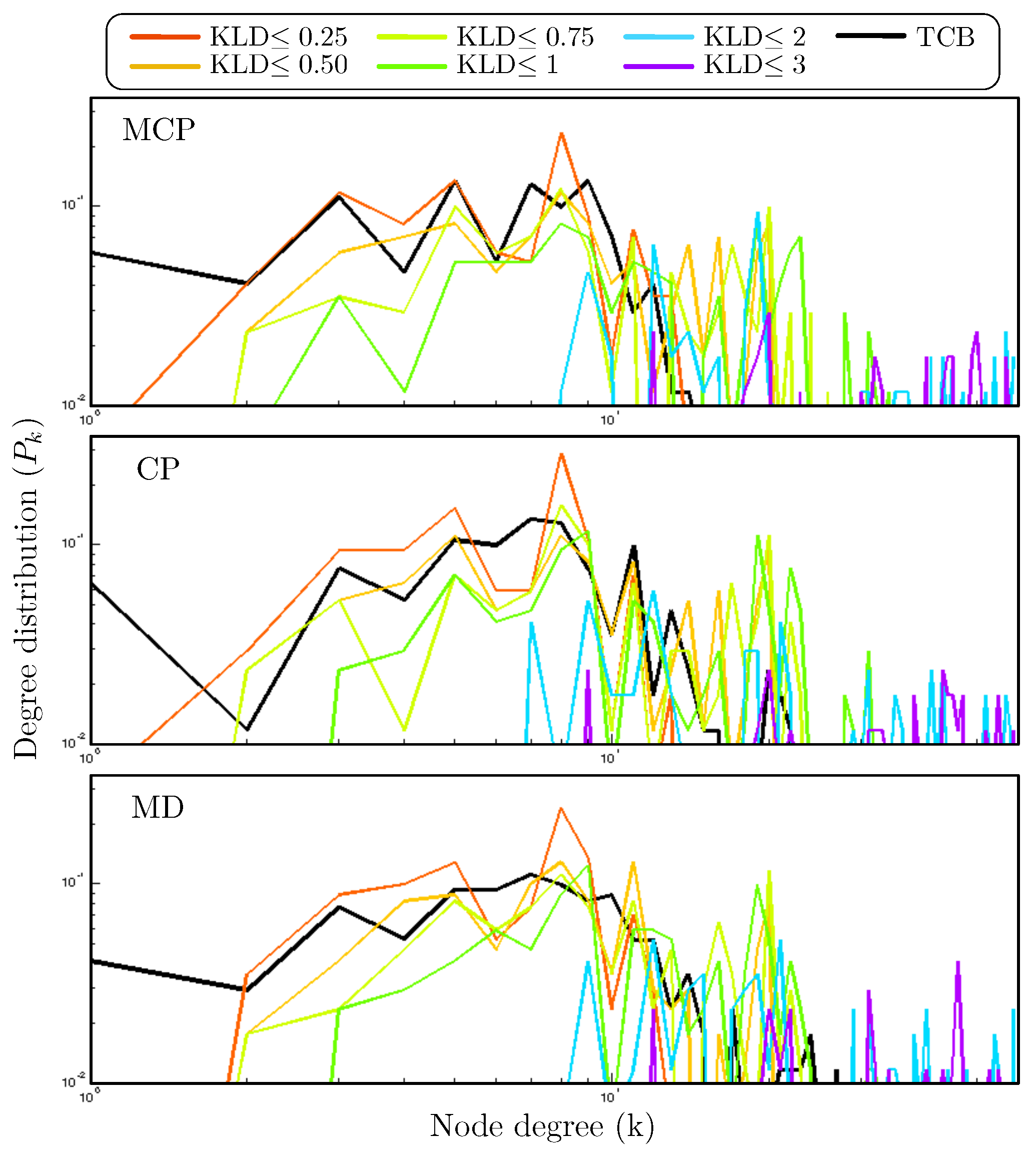
Figure 3 shows that the resulting degree distribution $P_k$ for both the proposed CN construction methodology and the TCB method are similar, mainly when low values for the KLD upper bound are considered. This fact suggests that the individual connectivity of the nodes is quite similar irrespective of the method used to construct the CN. Note that with the proposed method there are some nodes in the network with high degrees, especially for network constructed using large values for the KLD threshold. Thus, this detail reveals that CN constructed using low KLD values are related to the heterogeneous geographical distribution of the wind farms, which is something that the TCB method also does. However, large values of the KLD threshold are associated with connections between sub-networks, resulting in large networks with a high level of connections among nodes.

We continue studying the differences between the SODCC based and TCB construction methods by analyzing higher-order organization measures in the obtained networks. For this, it is interesting to analyze the appearance of nodes communities [49] in the considered CNs, fact that reveals geographical zones that are closely related. Different network’s measures detect these communities, such as the edge between centrality [50] or the edge clustering coefficient [51]. The latter is the generalization of the edges of the (vertex) clustering coefficient [52], a parameter widely used to measure the node tend to cluster together. In this work, we consider the local clustering coefficient distribution in order to obtain an indirect measure of the emergence and stability of clusters and communities using both SODCC based and the TCB based CN construction methods.

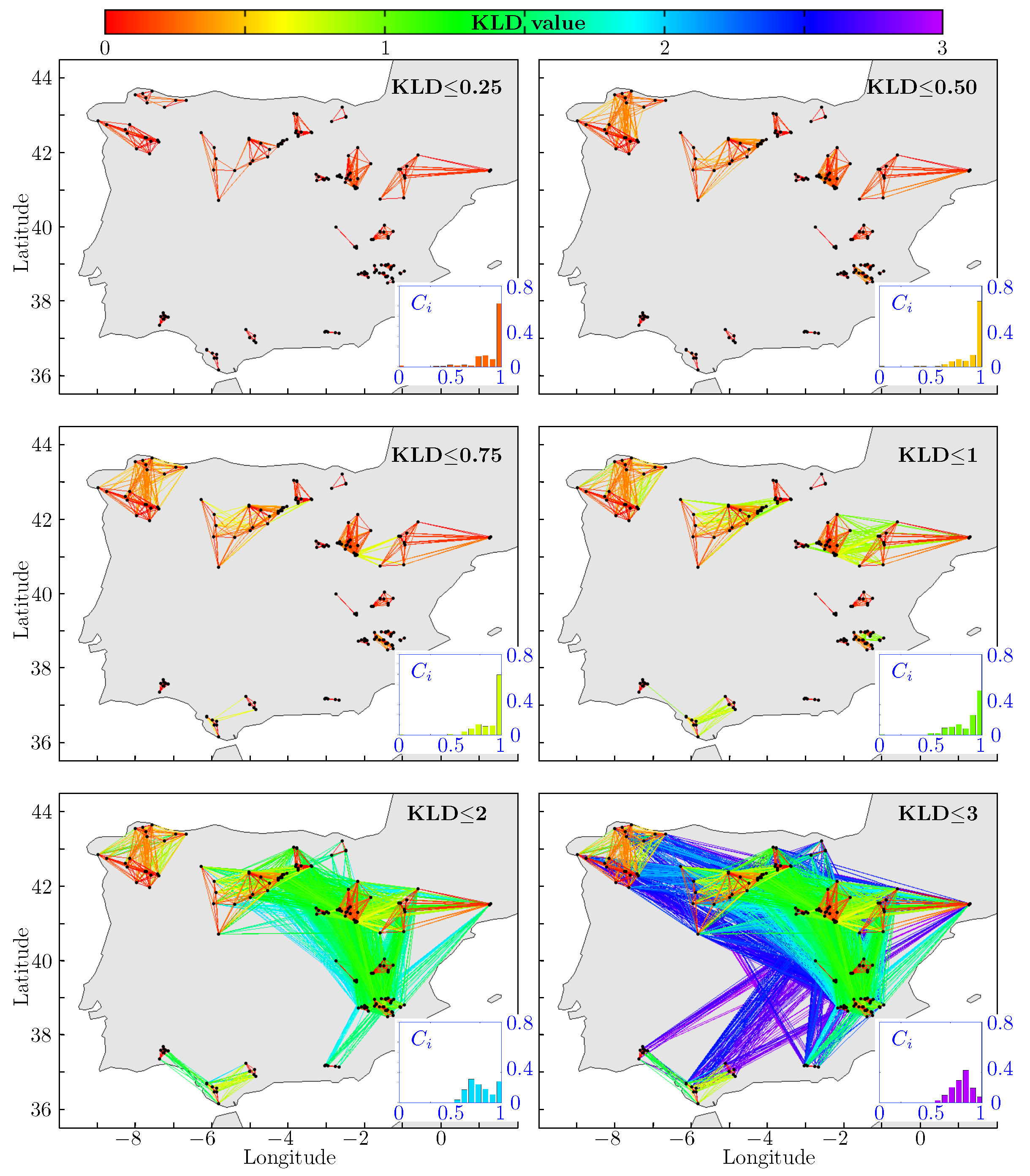
Figure 4, Figure 5 and Figure 6 show different CN obtained using the proposed methods and considering different KLD thresholds (KLD $\in \{0.25,0.50,0.75,1,2,3\}$) for the MCP, CP and MD time-horizons, respectively. These KLD thresholds are considered in order to clarify the relationship between the KLD value and both the connection inside the communities (lower values of KLD) and the connection among communities (higher values of KLD). The clustering coefficients ($C_i$) distributions for each CN are represented as an inset to each figure. Note that the color of the histogram is directly related to its corresponding KLD threshold.

These figures clearly show the hierarchical network structure ordering. For KLD $\le 0.25$, for all time-horizons, we can observe 20 disconnected sub-networks or communities, spatially localized. As the threshold in KLD is increased, the sub-networks connect among themselves. The $C_i$ clearly reflects this change in its distribution: it flattens as the KLD increases. However, a marked shape change does not occur up until a value of KLD $=2$ is reached. This is clearly related to the sparse connection among these sub-networks.

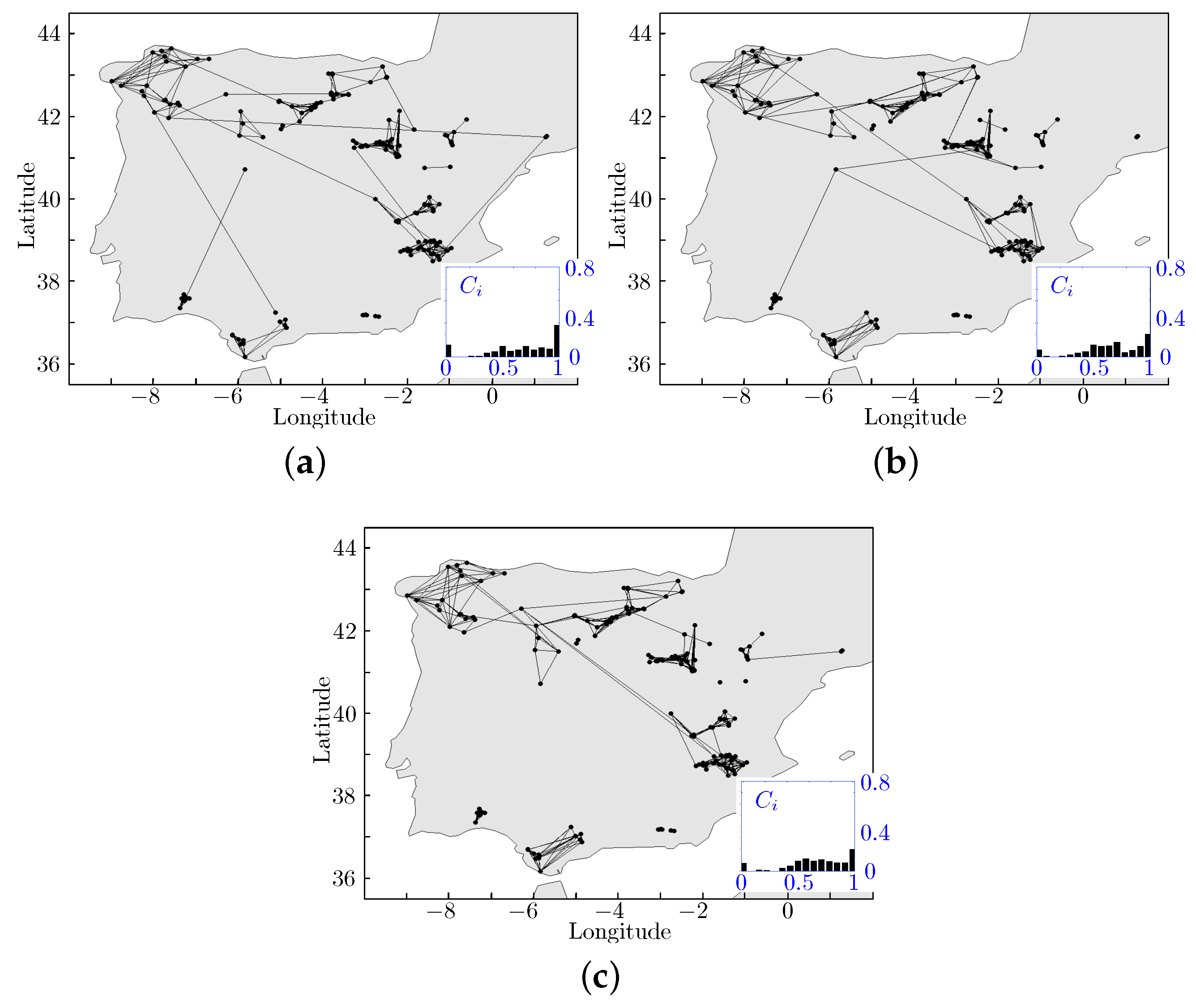
On the other hand, for comparison purposes, Figure 7 and Figure 8 show the obtained CNs using the TCB construction method with the parameter $u=2$ (which controls the statistical threshold $S^{th}$ of the link strength) and for two physically meaningful spatial thresholds $d^{th}=300$ km (mesoscale) and $d^{th}=1000$ km (synoptic scale). Also, the clustering coefficients $C_i$ for the corresponding CN are presented in the inset.

Regarding the consistency of the hierarchical CN obtained with the proposed method, we can see in Figure 4, Figure 5 and Figure 6 that the obtained communities for both the mesoscale (KLD $\le 1$) and synoptic scale (KLD $>1$) cases show approximately the same structure, regardless the considered time-horizon (MCP, CP or MD). Both the communities structure (red edges) and their interconnections (green, blue and violet edges) possess the same organization level. This finding is corroborated with the corresponding clustering coefficient distributions as they consistently show mono-modal distributions with maxima that evolve from $C_i\approx 1$ for low KLD thresholds to $C_i\approx 0.75$ for KLD $\in \{2,3\}$. Recall that this result seems to be independent of the considered prediction time-horizon.

On the other hand, for the CNs obtained with the TCB method and represented in Figure 7, closely located nodes show a consistent connectivity, but inter-community connectivity varies with the prediction time-horizon. It is worth noting that with this TCB method, the mesoscale relationship between the nodes is forced by means of the spatial threshold $d^{th}=300$ km in this case. If such a limitation is removed by increasing the spatial threshold (e.g., $d^{th}=1000$ km represented in Figure 8), the inter-community connectivity becomes much more erratic, thus pointing to the creation of spurious edges. This type of connections are not representative of actual data correlations. On top of the inconsistency of the inter-community connectivity, we can clearly see that the apparent similarity for the degree distribution $P_k$ previously analyzed (see Figure 3) is not preserved any more. The $C_i$s obtained for identical time-horizon obtained for both methodologies are noticeably different.

3.3. Physical Interpretation of the Obtained Results

As it can be observed in the proposed CN construction method based on the SODCC algorithm, it is self-consistent in space and time, i.e., the node communities and their respective interconnections are similar in shape and organization, irrespective of the considered prediction time-horizon.

Furthermore, with the selection of a given KLD threshold (KLD $<1$), analysis can be focused on the extraction of the mesoscale organization of the data from the nodes, thus revealing the mesoscale physics of the problem. For higher KLD values, the inter-community connectivity reveals the synoptic scale organization of the prediction error of the wind speed. In contrast, the CNs obtained with the TCB methodology reveal some local organization of the mesoscale, but it fails to extract the relationship between communities, giving way to the creation of spurious relations or the deletion of relevant ones, depending on the analyzed time-horizon.

Note that, in the specific problem of wind speed prediction error, the networks obtained give an idea of the relationships between wind farms with a similar structure in terms of prediction quality of the mesoscale numerical model, the WRF in this case. Thus, we can spot the nodes of the network (wind farms) in which the WRF works similar, and those in which the prediction is statistically different, due to orographic or other differences between wind farms. Note that we could use the WRF output in one wind farm to estimate the wind speed in the other one, since in both cases this prediction is similar according to the CN construction with the SODCC algorithm.

The mesoscale physics of the problem revealed by the CN obtained in this work can be further analyzed by comparing the results obtained (in terms of the constructed CN) with that of previous clustering approaches over wind speed data in the Iberian Peninsula (IP). Specifically, two recent works have obtained wind speed clusters over the IP [53,54]. In [53] the authors obtain a clustering approach with 20 wind clusters over the IP, extracted using a combination of hierarchical clustering and k-means methods, from the analysis of data from 868 automated weather stations distributed over the IP and Balearic Islands. The study on [54] uses reanalysis data (ERA-Interim) and a k-means algorithm to obtain a clustering of wind speed with 10 clusters over the IP.

Apart from the number of clusters considered, both studies obtain quite similar regions (clusters) for the wind speed in the IP (as expected), which, following [53], are produced by the complex orography of the IP, mainly valleys, delimited by mountain barriers, coastlines and plateaus. The idea is to compare the CNs of wind speed errors, obtained with the proposed method based on SODCC and KLD, with the clustering analysis of wind speed given by [53,54]. As it can be seen, the sub-networks formed for low values of thresholds in the KLD match with specific clusters given in [53,54].

For example, choosing the work [53] as a reference (see Figure 9), the sub-networks of wind speed error obtained with the KLD approach are fully consistent with [53] clusters R13 (Galicia), R8 and R16 (Huelva and Cádiz), R3 (Castilla-León), R6 (Basque Country), R4 and R7 (Southern Catalonia and Aragón) and R5 and R10 (South-East of Castilla la Mancha). In other words, these results show a clear relationship between the wind cluster in which the wind farm is located in the IP, and the wind speed error obtained with the mesoscale model considered in this study (WRF model). This can be associated with a different orography existing in each zone, which produces a different behaviour of the mesoscale model in each cluster area. As shown, the proposed CN construction method has been able to locate this specific zones with different performance of the mesoscale model for wind speed prediction. However, contrary to our approach, it cannot quantify the similarity among the obtained clusters.

Finally, it is to be remarked that the construction of the resulting climate networks facilitate the identification of their symmetry properties. It has been shown that the identification of the essential network symmetries and use these symmetries to derive natural direct product decomposition of the automorphism group into irreducible factors [35] are critical to extract the relationship between network symmetry and redundancy. The redundancy in climate networks can help identify similar behaviors in different parts of the networks and capture similarities. The hierarchy induced by the resulting communities for decreasing KLD make the identification of the irreducible factors very obvious and, thus, the redundancies are also clearly seen. Another kind of complex network symmetry, the so called stochastic graph symmetry [36,37], is a stochastic version of link reversal symmetry, which leads to an improved understanding of the reciprocity of directed networks. Because of the statistical nature of the links in the present complex networks, it makes quite easy to construct a version of a directed network. By examining the symmetry breaking process in those directed networks, underlying mechanisms can be identified. This will be the subject of future works.

4. Conclusions

The appearance of spurious and missing links are two important problems when constructing CNs as correlation networks. In this paper we have proposed a new methodology for CN construction using the SODCC algorithm and the KLD metric between MP distributions. The proposed method is able to construct CNs with fewer spurious links and more self-consistence in space and time compared to the TCB method. We have evaluated the performance of the proposed method using wind speed prediction error data from wind farms in Spain. We have shown that the proposed approach produces mesoscalar CNs with an emergent behaviour in terms of different network measures such as degree distribution and clustering coefficient, obtaining better performance than TCB approaches, which produce spurious and missing links.

We have shown that physical mesoscale relationships persist after the removal of the WRF model predictions from the measured wind speed (error calculation). Furthermore, by using of the KLD metric over the SODCC results, we are able to construct a continuous measure of similarity among the different regions that is consistent in time. This fact provides a methodology to consistently evaluate the error in wind speed prediction models, that classical CN construction by means of direct correlation between time series is not able to give.

In future works we will evaluate the proposed method for construction of global climate networks of atmospheric variables, affected by phenomena such as global patterns of teleconnections or atmospheric events such as Rossby waves or the ENSO phenomenon.