Article

Multi Body Dynamic Equations of Belt Conveyor and the Reasonable Starting Mode

School of Mechatronic Engineering, JiangSu Normal University, Xuzhou 221116, China
*
Author to whom correspondence should be addressed.
Symmetry 2020, 12(9), 1489; https://doi.org/10.3390/sym12091489
Submission received: 13 August 2020 / Revised: 1 September 2020 / Accepted: 8 September 2020 / Published: 10 September 2020

Abstract

:
Based on the rigid finite element method and multibody dynamics, a discrete model of a flexible conveyor belt considering the material viscoelasticity is established. RFE (rigid finite element) and SDE (spring damping element) are used to describe the rigidity and flexibility of a conveyor belt. The dynamic differential equations of the RFE are derived by using Lagrange’s equation of the second kind of the non-conservative system. The generalized elastic potential capacity and generalized dissipation force of the SDE are considered. The forward recursive formula is used to construct the conveyor belt model. The validity of dynamic equations of conveyor belt is verified by field test. The starting mode of the conveyor is simulated by the model.

1. Introduction

Belt conveyors are widely used in the field of transportation engineering due to their advantages of a strong conveying capacity, a long conveying distance, high speed, stable operation and low noise [1]. A typical belt conveyor is composed of conveyor belts, drive rollers, redirecting rollers, idlers, tensioning devices and braking devices. It is a complex long-distance rigid-flexible coupling mechanical system. Therefore, the establishment of an easy-to-solve and accurate calculation system model has significant engineering significance for the analysis of the dynamic performance of a conveyor and the prediction of fatigue damage [2,3]. The core component of a conveyor—the material of a conveyor belt—has relatively good mechanical properties. It cannot be treated simply as a rigid or elastic body [4]. The model that closely resembles its essential characteristics is the viscoelastic model [5,6], which makes the dynamic analysis model of the conveyor belt much more complex than that of general mechanical parts. The dynamic analysis model of conveyor belt mainly includes continuous model and discrete model. The continuation model refers to the various dynamic differential equations commonly used by early researchers studying belt conveyors [7]. The establishment of these models promotes the improvement of the design of belt conveyors. However, the differential equations for the boundary conditions and initial conditions have become more complex. Discrete models are derived from continuous models. The modeling accuracy and engineering application value are continuously improved [8,9].
The earliest finite element discrete model is a one-dimensional longitudinal vibration analysis model [10,11], which is essentially based on the concentrated mass finite element method. It regards the continuous conveyor belt as a system composed of a series of particles connected by springs and damping elements. The quality and force of the conveyor belt, including the mass of the bulk material, the running resistance of the rollers, etc. [12,13], are concentrated at a node. The dynamic equations of the entire system are linear differential equations. This type of model has achieved good results in the longitudinal vibration analysis of a conveyor belt. Li [14] used the Kelvin–Voigt viscoelastic model to establish continuous dynamic equations for tail hammer tension belt conveyors. Various factors influencing the longitudinal vibration of the belt conveyor were simulated. The two-dimensional finite element model mainly refers to the mixed finite element model of rod and beam elements [15]. This method can comprehensively consider the coupling problem associated with the longitudinal and lateral vibrations of a conveyor belt. To investigate belt deflection for variable dynamic conditions, Shen [16] developed a coupled finite element method (FEM) and discrete element method (DEM) model to predict the dynamic belt deflection. Ilic [17] established a conveyor belt model with the DEM to study the interaction between bulk solids and the belt during transportation. There was a good correlation between the experimental data and the simulation results. The calculation method of the conveyor roller load has improved.
Although the finite element method has achieved great success in the analysis of the longitudinal and transverse vibration characteristics of a conveyor belt, in essence, the various belt conveyor dynamic analysis methods based on the finite element method still belong to the structural dynamic analysis. Most existing models do not fully consider the nonlinear problem of conveyor belts. The flexible conveyor belt exhibits viscoelasticity in terms of mechanical properties. During the working process, there is a relatively large deformation relative to other parts. This coupling of large displacement, large deformation and viscoelasticity on the conveyor belt makes the nonlinear problem in its dynamic analysis very prominent. Many researchers use a variety of relatively simple linear models to study the dynamic characteristics of belt conveyors, which will inevitably have an adverse effect on the accuracy of its analysis. The dynamic analysis method for a belt conveyor system must still be established based on the multibody system dynamics method.
The rigid finite body element method is a flexible multibody dynamic analysis method based on the theory of multibody dynamics. It divides the flexible or rigid flexible multibody system into a series of rigid finite elements (RFE) connected by spring damping elements (SDE). The main difference between the RFE method and the FE method is that the RFE method uses a rigid finite body element to describe the inertia forces of a flexible body. The element flexibility is described relative to the rigid body element’s conjoined coordinate system, instead of the flexible body’s body coordinate system. The small deformation between rigid body elements is used to describe the large deformation of the entire flexible body. This naturally takes into account the geometric nonlinearity effects of the dynamic stiffness, without the need for a geometric stiffness matrix. Flexible multibody systems and rigid-flexible hybrid multibody systems can be handled in a unified way. Nonlinear spring damping element parameters can be used to conveniently solve material nonlinearity problems. For example, the relationship between the rolling resistance of a roller and the parameters of the equipment system can be described using spring damping elements [18]. Therefore, the rigid finite body element method is particularly suitable for the computer simulation modelling of a rigid-flexible complex mechanical system composed of a flexible body (conveyor belt) and a rigid body (roller, roller system, etc.), such as a belt conveyor.
In this paper, a flexible multibody dynamic model of a conveyor belt is established based on the RFE method. The model is used to study the dynamic performance of the conveyor under different starting modes.

2. Rigid Finite Element Model of a Conveyor Belt

2.1. Discrete Model of the Conveyor Belt

As shown in Figure 1, a conveyor system consists of p-1 parts and conveyor belt p. The conveyor belt p can be discretized into mp rigid body elements (RFEs) reflecting the rigid characteristics of the conveyor belt, and the rigid body elements are connected by spring damping elements (SDE) reflecting the flexible characteristics of the conveyor belt. Then, the whole conveyor system is simplified into a rigid flexible multi-body system composed of p-1 rigid bodies, mp RFEs and mp SDEs. The simplified dynamic model of conveyor belt is symmetrical in structure.

2.2. Coordinate Description

2.2.1. Rigid Finite Element

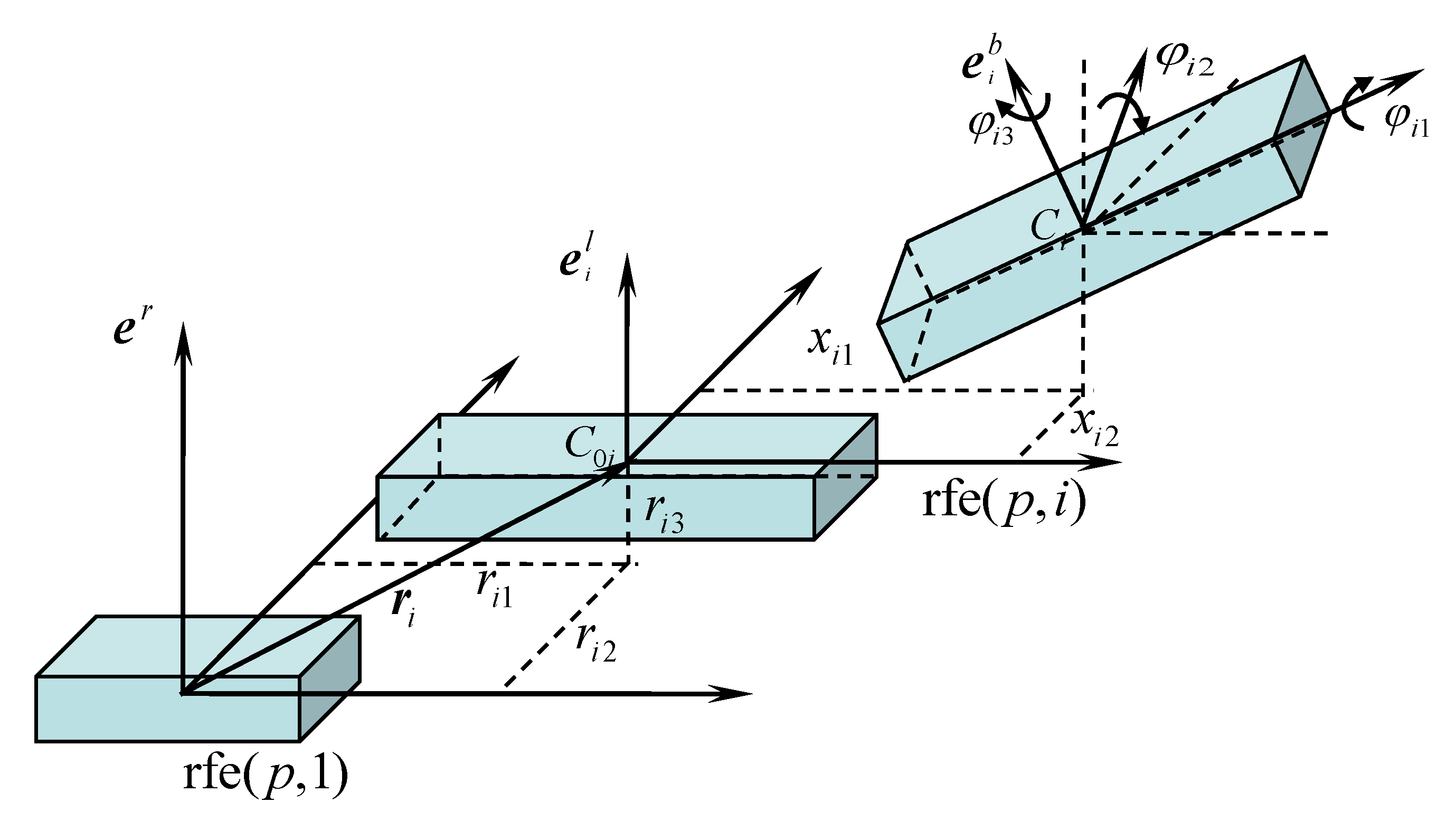
Figure 2 shows the coordinate system of the RFE of the conveyor belt. It includes the reference coordinate system e r , local coordinate system e i l and floating coordinate system e i b of the RFE (p, i) [19].
The reference coordinate system e r is selected at the first RFE (p, 1), and each RFE has a local coordinate system e i l . The elastic displacement of the RFE (p, 1) is described by the position and altitude of e i l relative to e r before belt deformation. The origin of e i l is at the initial position C 0 i of the centroid of the RFE. The three coordinate axes coincide with the main inertia axis. Before deformation, the floating coordinate system e i b coincides with the local coordinate system e i l and moves with the RFE.
The constant transformation matrix from the local coordinate system e i l of the RFE (p, i) to the reference coordinate system e r is as follows:
B i r l = [   A i r l r i 0 1 ]
where A i r l is the direction cosine matrix of e i l with respect to e r , and r i is the coordinate vector of the origin of e i l in e r .
Unlike rigid bodies, the conveyor belt is elastic, and the relative positions of various points in the body are constantly changing. Therefore, the position and altitude of the floating coordinate system e i b relative to the local coordinate system e i l can be described by the following generalized coordinates:
q i b = [ x i 1 x i 2 x i 3 φ i 1 φ i 2 φ i 3   ] T = [ x i φ i ]
where x i is a coordinate vector of the origin of e i b in e i l , and φ i is an altitude coordinate vector of e i b in e i l .
According to the above equation, the transformation matrix of e i b to e i l for RFE (p, i) is:
B i l b = [   A i l b x i 0 1 ]
where,
A i l b = [   C i 1 C i 3 S i 1 C i 2 S i 3 C i 1 S i 3 S i 1 C i 2 C i 3 S i 1 S i 2 S i 1 C i 3 + C i 1 C i 2 S i 3 S i 1 S i 3 + C i 1 C i 2 C i 3 C i 1 S i 2 S i 2 S i 3 S i 2 C i 3 C i 2 ]
where, C i 1 = cos φ i 1 , S i 1 = sin φ i 1 .
Therefore, the uniform transformation matrix of e i b to e r for RFE (p, i) is:
B i r b = B i r l B i l b

2.2.2. Spring Damping Element (SDE)

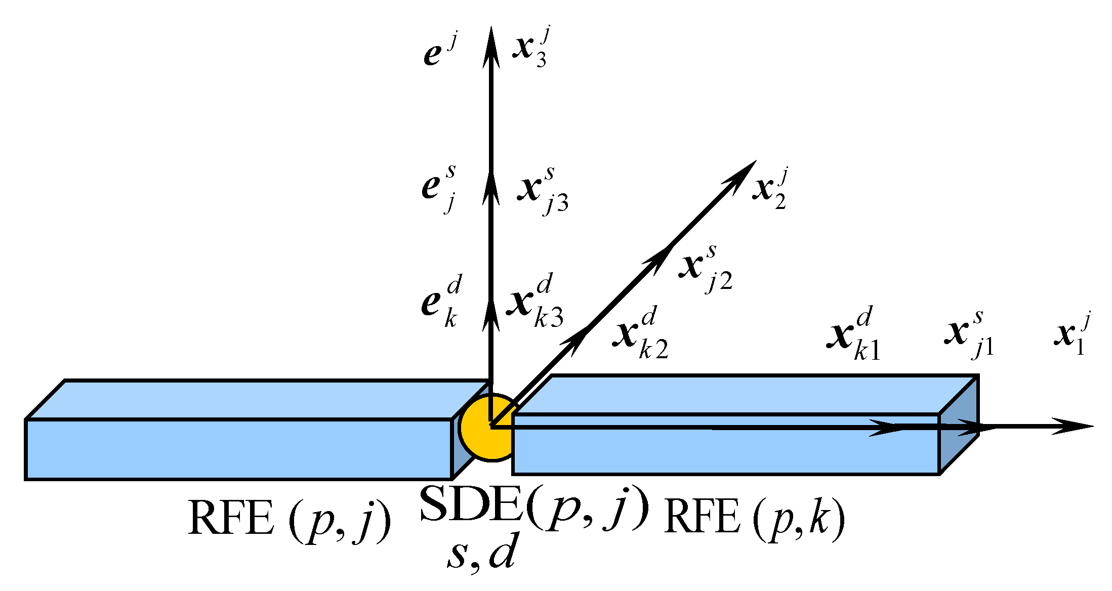
The deformation of the conveyor belt caused by external and inertial forces is described by the SDE. The coordinate system of SDE (p, j), connecting RFE (p, j) and RFE (p, k), is shown in Figure 3. To describe the flexible characteristics of the conveyor belt, a local coordinate system e j is established at SDE (p, j) before its deformation. Coordinate systems e j s and e k d are established at the connection points s (between RFE (p, j) and SDE (p, j)) and d (between RFE (p, k) and SDE (p, j)), respectively. The three coordinate systems are now coincident.
The positions and altitudes of the SDE (p, j) coordinate system e j at the local coordinate systems e j l and e k l of RFE (p, j) and RFE (p, k) are represented by the following constant transformation matrices:
B j l j = [   A j l j x j j 0 1 ]
B k l j = [   B k l j x k j 0 1 ]
It should be noted that the constant transformation matrices of the coordinate systems e j s and e k d at points s and d with respect to their respective floating coordinate systems are equal to the above equations. Due to the load on the conveyor belt, RFE (p,j) and RFE (p,k) will produce elastic deformation. Therefore, the position and altitude of the floating coordinate system e i b relative to the respective local coordinate systems e j l and e k l can be described by the generalized coordinate given in Equation (2):
q j b = [ x j 1 x j 2 x j 3 φ j 1 φ j 2 φ j 3 ] T = [ x j φ j ]
q k b = [ x k 1 x k 2 x k 3 φ k 1 φ k 2 φ k 3 ] T = [ x k φ k ]
From Equations (6) and (7), and considering Equation (3), the position coordinate vectors of points s and d relative to their respective local coordinate systems e j l and e k l can be calculated by the following equation:
x j s = A j l b x j j + x j
x k d = A k l b x k j + x k
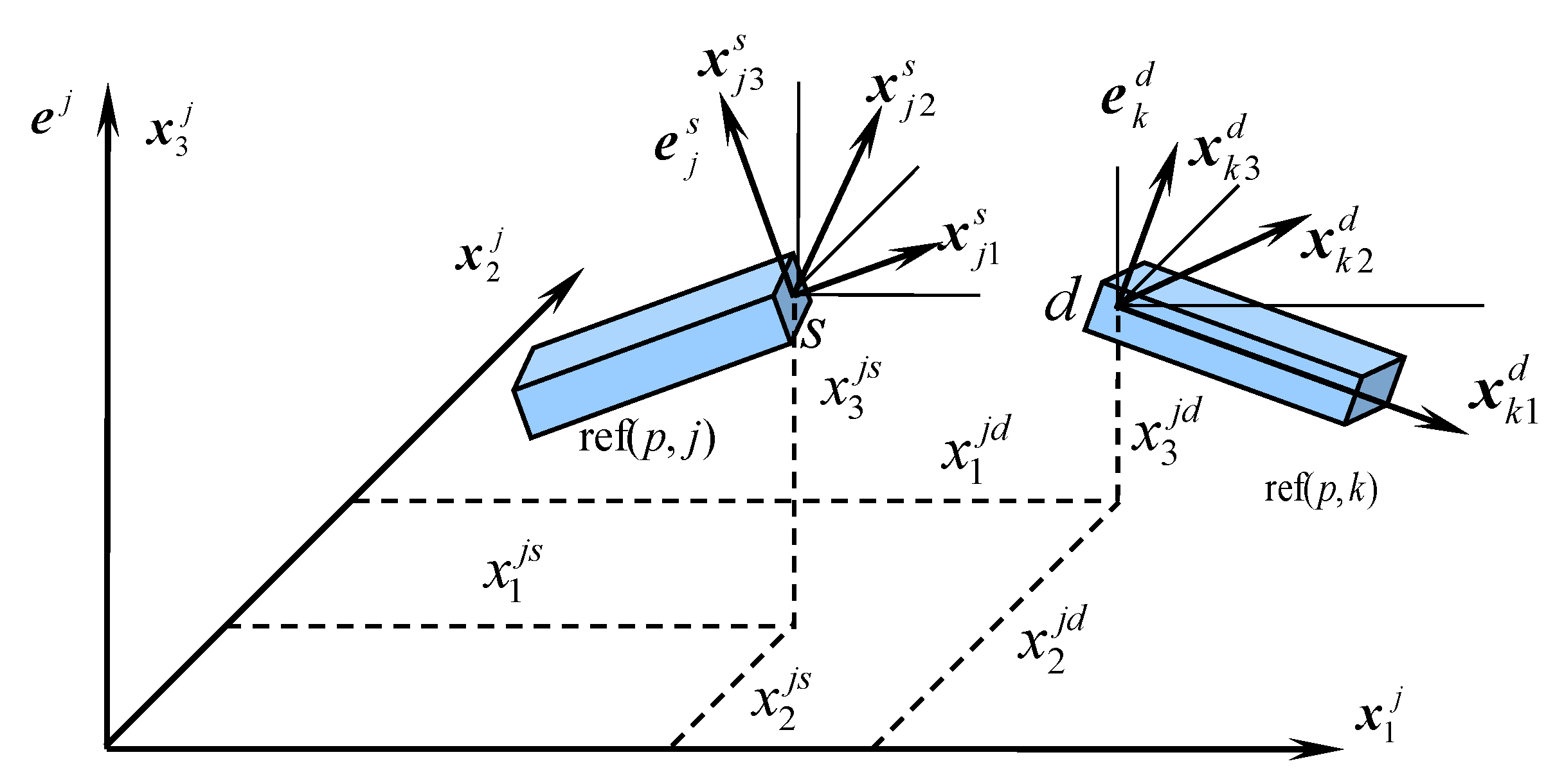
Considering Equation (6) and its inverse matrix, from Equation (8), the position coordinate vector of points s and d relative to the SDE (p,j) coordinate system e j can be obtained (Figure 4):
x j s = [ A j l j ] T [ ( A j l b I ) x j j + x j ]
x j d = [ A k l j ] T [ ( A k l b I ) x k j + x k ]
From the above equation, the relative displacement matrix of points s and d at SDE (p,j) caused by the deformation of the conveyor belt can be obtained:
Δ x j = x j s x j d
Similarly, the relative rotation angular displacement matrix is:
Δ φ j = φ j s φ j d

2.3. Spring Damping Element Parameters

2.3.1. Potential Energy and Generalized Stiffness Matrix

The potential energy of the SDE (p,j) is divided into two terms. One is caused by the displacement changes between elements j and k:
V x j = 1 2 [ Δ x j ] T C x j Δ x j
The other term is caused by the rotation change:
V φ j = 1 2 [ Δ φ j ] T C φ j Δ φ j
where Δ x j and Δ φ j are defined by Equations (10) and (11). C x j and C φ j are generalized stiffness matrices:
C x j = [ c x 1 j 0 0 0 c x 2 j 0 0 0 c x 3 j ] ,   C φ j = [ c φ 1 j 0 0 0 c φ 2 j 0 0 0 c φ 3 j ]
where c x i j and c φ i j are the translation stiffness coefficient and rotation stiffness coefficient, respectively.
Then, the total elastic potential energy of SDE (p,j) is:
V j = V x j + V φ j = 1 2 [ Δ x j ] T C x j Δ x j + 1 2 [ Δ φ j ] T C φ j Δ φ j
Similarly, the total energy loss function of SDE (p, j) is:
W j = W x j + W φ j = 1 2 [ Δ x ˙ j ] T D x j Δ x ˙ j + 1 2 [ Δ φ ˙ j ] T D φ j Δ φ ˙ j
where D x j and D φ j are generalized damping matrices. Δ x ˙ j and Δ φ ˙ j are relative moving and rotation rate matrices which can be derived by Equations (10) and (11).

2.3.2. Coefficients of the Stiffness and Damping

The parameters of the SDE include stiffness coefficients c x i j and c φ i j and damping coefficients d x i j and d φ i j . These coefficients will determine the flexible characteristics of the flexible body, and the values of the coefficients are determined by the mechanical model and the section shape of the RFE. For conveyor belts with viscoelastic mechanical properties, the following assumptions are made:
  • Each RFE can be simplified into an equal length beam element with a rectangular section shape;
  • The deformation mode and velocity of the actual conveyor belt are the same as that of its equivalent SDE;
  • The stress of each section in the conveyor belt section is equal, and its mechanical properties can be described by the Voigt model [20]:
σ ( t ) = E ε ( t ) + η ε ˙ ( t )
where σ ( t ) is the belt stress, ε ( t ) is the belt strain, ε ˙ ( t ) is the strain rate, E is the Elastic modulus, and η is the viscosity coefficient.
Based on the above assumptions, the following relationships can be obtained:
σ ( t ) = F 1 ( t ) A ε ( t ) = Δ w 1 ( t ) Δ l ε ˙ ( t ) = Δ w ˙ 1 ( t ) Δ l
where F 1 ( t ) is the tension of the belt element, Δ w 1 ( t ) is the longitudinal deformation of the belt element, Δ w ˙ 1 ( t ) is the longitudinal deformation rate of the belt element, A is the cross-sectional area of the belt element, and Δ l is the belt element length.

2.4. Rigid Finite Element Parameters

2.4.1. Kinetic Energy and Lagrangian Operator

There are two kinds of simplified rigid bodies that can be used when modelling rigid flexible hybrid multibody systems or flexible multibody systems with the rigid finite body element method. One is the natural rigid body, that is, the actual object whose elastic deformation is negligible compared with that of other objects in the system. The other is the RFE formed after the discretization of the flexible body, which must be considered after deformation. Although these two kinds of rigid bodies have different choices for generalized coordinates, the method of establishing the kinematic equation is the same. In order to simplify the derivation process, the two kinds of rigid bodies will not be distinguished. The generalized coordinates of a rigid body in the system are uniformly expressed as follows:
q = [ q 1 q k q n ] T
where q k is the generalized coordinate component.
The dynamic differential equations of a rigid body given by Lagrange’s equations of the second kind for a nonconservative system are [21]:
d d t T q ˙ k T q k + V q k = Q k ( k = 1 , , n )
where T is the kinetic energy, V is the potential energy, including the gravitational energy and elastic energy, q ˙ k is the generalized velocity component, and Q k is the generalized force components of nonconservative systems. The Lagrange operator is:
ε k ( T ) = d d t T q ˙ k T q k
The matrix form of Equation (18) is:
ε q ( T ) + V q = Q
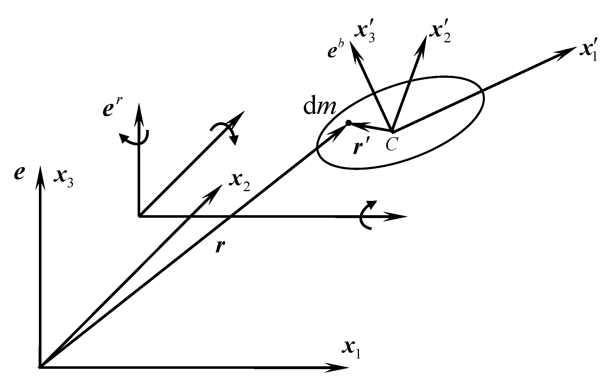
As shown in Figure 5, the mass of a particle on a rigid body is d m , and the position vector diameter in the rigid body connected coordinate system e b is r . In the global coordinate system, the vector of e is r . e r is a moving reference frame. For a natural rigid body, e r is the coordinate system between adjacent bodies. For rigid elements of a flexible body, e r is the coordinate system of the starting rigid element.
Then, the relationship between the position and diameter of a particle in different coordinate systems can be expressed as:
r = B r B r b r = B b r
where,
r = [ x 1 x 2 x 3 1 ] T is the coordinate matrix for a particle in the rigid body coordinate system e b ;
r = [ x 1 x 2 x 3 1 ] T is the coordinate matrix for a particle in the global coordinate system e .
B b is the uniform transformation matrix of the rigid body coordinate system e b relative to global coordinate system e , which is abbreviated as B .
Then, the kinetic energy of a rigid body is:
T = 1 2 m t r ( r ˙ r ˙ T ) d m = 1 2 m t r ( B ˙ r r T B ˙ T ) d m = 1 2 t r [ B ˙ ( m r r T d m ) B ˙ T ] = 1 2 t r [ B ˙ H B ˙ T ]
where H is the so-called pseudo inertia matrix at the origin C of the rigid body relative coordinate system e b .
Equation (23) can be obtained by substituting Equation (22) into Equation (19) and omitting the derivation process:
ε k ( T ) = t r { B k H [ B ¨ r B r b + 2 B ˙ r B ˙ r b + i = 1 n j = 1 n B i , j q ˙ i q ˙ j + i = 1 n B i q ¨ i ] T } = i = 1 n a k i q i + e k ( k = 1 , , n )
where,
B k = B q k = B r B r b q k ,   B k , j = B k q j = B r B r b q k q j = B j , k ,   B ˙ r b = j = 1 n B r b q j q ˙ j , a k , i = t r ( B k H B i T ) ,   e k = t r { B k H [ B ˙ r B r b + 2 B ˙ r B ˙ r b + i = 1 n j = 1 n B i , j q ˙ i q ˙ j ] T }
Equation (23) can be written in matrix form as:
ε q ( T ) = A q ¨ + e
where A = ( a k , i ) k , i = 1 , , n and e = ( e k ) k = 1 , , n

2.4.2. Gravitational Potential Energy and Generalized Force

If the mass of the rigid body element is m , gravity is g , and the vector diameter of the rigid body centre in coordinate system e b is expressed by r C , then the gravitational potential energy can be calculated as:
V g = m g θ 3 B r C
where θ 3 = [ 0 0 1 0 ] is the transformation matrix. Matrix B is the same as that the above section.
Deriving the generalized coordinate q k for the rigid body from the above equation gives:
V g q k = m g θ 3 B k r C ( k = 1 , , n )
Equation (26) written in matrix form is:
V g q = g
where g = ( g k ) k = 1 , , n   and g k = m g θ 3 B k   r   C If the coordinate matrix of the external force P acting on a point on the rigid body in coordinate system e b is P and the coordinate matrix of the position vector is r , then the generalized force corresponding to the generalized coordinate q k of the rigid body is:
Q k ( P ) = P T B T B k r
If the coordinate matrix of the external force couple M acting on the rigid body in coordinate system e b is:
M = [ M 1 M 2 M 3 0 ] T
Then, the generalized force corresponding to the generalized coordinate q k of the rigid body is:
Q k ( M ) = M 1 l = 1 3 b l , 3 b k , l , 2 + M 2 l = 1 3 b l , 1 b k , l , 3 +   M 3 l = 1 3 b l , 2 b k , l , 1
The generalized force matrix of the rigid body is:
Q = ( Q k ) k = 1 , , n ,   Q k = Q k ( P ) + Q k ( M )
Substituting Equations (24), (27), and (31) into Equation (18), the dynamic equation of the rigid body can be obtained as follows:
A q ¨ = F
where F = Q e g .

2.4.3. Elastic Potential Energy

For a flexible body such as a conveyor belt, its deformation is described by a spring damping element. Therefore, the dynamic equation of the rigid body element should also include the generalized force term corresponding to the potential energy caused by elastic deformation. From Section 2.3, the elastic deformation potential energy of SDE (p, j) connecting RFE (p, j) and RFE (p, k) of flexible body p is:
V ( p , j ) = V x ( p , j ) + V φ ( p , j ) = 1 2 [ Δ x ( p , j ) ] T C x ( p , j ) Δ x ( p , j ) + 1 2 [ Δ φ ( p , j ) ] T C φ ( p , j ) Δ φ ( p , j )
Then, the total elastic potential energy of the flexible body p can be obtained from the sum of the elastic deformation potential energy of all m p spring damping elements. Then, the total elastic potential energy of p can be calculated from the sum of the potential energy of all m p SDEs:
V ( p ) = j = 1 m p V ( p , j )
The generalized force corresponding to the generalized coordinate q ˜ ( p , k ) of RFE (p, k) can be defined by the following equation:
v ( p , k ) = V ( p ) q ˜ ( p , k ) = j = 1 m p v ¯ ( j , k )
The generalized elastic potential capacity matrix corresponding to all the generalized coordinates q ˜ ( p ) of the flexible body p can be written as:
v ( p ) = V ( p ) q ˜ ( p ) = [ v ( p , 1 ) v ( p , i ) v ( p , m p ) ]
Similarly, the generalized dissipative force matrix corresponding to all generalized coordinates q ˜ ( p ) of p is:
w ( p ) = W ( p ) q ˜ ( p ) = [ w ( p , 1 ) w ( p , i ) w ( p , m p ) ]

2.5. Multibody Dynamic Equation

2.5.1. Forward Recursive Formulation

Theoretically, the system’s equations of motion can be obtained by combining the dynamic equations of all the rigid bodies or elements in the system. However, the classical rigid finite element method uses two types of generalized coordinates for a rigid-flexible hybrid system (hinged Lagrange coordinates for the adjacent objects in the system and generalized coordinates of Cartesian and Euler angles for the rigid elements of the belt). Thus, the right term of dynamic Equation (42) for each object in the system’s motion chain and matrix A will contain the topological information of all the low-order bodies in its path. The form is quite complicated. Therefore, the dynamic equation of the entire system needs to be established using recursive groups, starting from the low-order body of the system [22].
Consider a system consisting of p 1 rigid bodies and flexible body p . To simplify the description, flexible body p is not initially discrete, and is treated in the same way as the rigid bodies. The generalized coordinate vector of the flexible body p in the global coordinate system and the transformation matrix of its local coordinate system to the global coordinate system can be expressed as:
q ( p ) = [ q ( 1 ) q ˜ ( k ) q ˜ ( p )   ] T = [ q ( p 1 ) q ˜ ( p ) ]
B ( p ) = B r B p r b = B r B p 1 r b B ˜ ( p ) = B ( p 1 ) B ˜ ( p )
where   q   ˜ ( p ) is the generalized coordinate vector of the flexible body p relative to the rigid body p 1 , which can be expressed by:
q ˜ ( p ) = [ q ˜ 1 ( p ) q ˜ n p ( p )   ] T
where, q ( p 1 ) is the generalized coordinate vector of the flexible body p adjacent to the low-order rigid body p 1 in the global coordinate system; B ˜ ( p ) is the transformation matrix of the local coordinate system of the flexible body p relative to the local coordinate system of the rigid body p 1 ; B ( p 1 ) is the transformation matrix of the rigid body p 1 in the local coordinate system relative to the global coordinate system.
Note that the number of generalized coordinates n p of the flexible body p is dependent on the number of generalized coordinates of all its low-order bodies and the number of generalized coordinates of itself relative to the adjacent low-order rigid body p 1 , i.e.,
n p = n p 1 + n ˜ p = k = 1 p n ˜ k
The dynamic equation of the flexible body p described by Equation (32) can be rewritten as follows:
A ˜ ( p ) q ¨ ( p ) = F ˜ ( p )
It can also be expanded into:
[ A ˜ 1 , 1 ( p ) A ˜ 1 , k ( p ) A ˜ 1 , p ( p ) A ˜ j , 1 ( p ) A ˜ j , k ( p ) A ˜ j , p ( p ) A ˜ p , 1 ( p ) A ˜ p , k ( p ) A ˜ p , p ( p ) ] [ q ˜ ¨ ( 1 ) q ˜ ¨ ( k ) q ˜ ¨ ( p ) ] = [ Q ˜ 1 ( p ) Q ˜ j ( p ) Q ˜ p ( p ) ] [ e ˜ 1 ( p ) e ˜ j ( p ) e ˜ p ( p ) ] [ g ˜ 1 ( p ) g ˜ j ( p ) g ˜ p ( p ) ]
Equation (41) reveals the relationship between the motion of the flexible body p and its own coordinates q ˜ ( p ) and the generalized coordinates of all its low-order rigid bodies. See Appendix A for details. The recursive relationship can be simplified as:
[ A ¯ p 1 , p 1 ( p ) A ¯ p 1 , p ( p ) A ¯ p , p 1 ( p ) A ¯ p , p ( p ) ] [ q ¨ ( p 1 ) q ˜ ¨ ( p ) ] = [ Q ¯ p 1 ( p ) Q ¯ p ( p ) ] [ e ¯ p 1 ( p ) e ¯ p ( p ) ] [ g ¯ p 1 ( p ) g ¯ p ( p ) ]
The kinetic energy T ( p ) and the gravitational potential energy V g ( p ) of the system can be derived from the sum of the kinetic and gravitational potential energy of all the objects in the system. The recursive relationship for energy is:
T ( p ) = k = 1 p T ˜ ( k ) = T ( p 1 ) + T ˜ ( p )
V g ( p ) = k = 1 p V ˜ g ( k ) = V g ( p 1 ) + V ˜ g ( p )
The dynamic equation of a system composed of p 1 rigid bodies can be written as:
A ( p 1 ) q ¨ ( p 1 ) = Q ( p 1 ) e ( p 1 ) g ( p 1 )
Then, the dynamic equation of the entire system composed of Equations (42) and (45) can be expressed as:
[ A ( p 1 ) + A ¯ p 1 , p 1 ( p ) A ¯ p 1 , p ( p ) A ¯ p , p 1 ( p ) A ¯ p , p ( p ) ] [ q ¨ ( p 1 ) q ˜ ¨ ( p ) ] = [ Q ( p 1 ) + Q ¯ p 1 ( p ) Q ¯ p ( p ) ] [ e ( p 1 ) + e ¯ p 1 ( p ) e ¯ p ( p ) ] [ g ( p 1 ) + g ¯ p 1 ( p ) g ¯ p ( p ) ]

2.5.2. Dynamic Equation of the Rigid Flexible Multibody System

If the abovementioned flexible body p is discretized into m p rigid body elements, the generalized coordinate vector describing the i-th rigid body element in the global coordinate system and the transformation matrix of its local coordinate system to the global coordinate system can be expressed by the following equation:
q ( p , i ) = [ q ( 1 ) q ˜ ( p 1 ) q ˜ ( p , 1 ) q ˜ ( p , i )   ] T = [ q ( p 1 ) q ˜ ( p , 1 ) q ˜ ( p , i ) ]
B ( p , i ) = B ( p , 1 ) B ˜ ( p , i ) = B ( p 1 ) B ˜ ( p , 1 ) B ˜ ( p , i )
Then, the number of generalized coordinates describing the motion of RFE (p, i) of the flexible body p can be expressed as:
n p , i = n p 1 + n ˜ p , 1 + 6 = n p , 1 + 6
The generalized coordinate vector of the entire flexible body p is expressed by the following equation:
q ( p ) = [ q ( p 1 ) q ˜ ( p , 1 ) q ˜ ( p ) ]
where,
q ˜ ( p ) = [ q ˜ ( p , 2 ) T q ˜ ( p , m p ) T ]
Then, the dynamic equation of the entire flexible body p can be expressed as:
[ A p 1 , p 1 ( p ) A p 1 , ( p , 1 ) ( p ) A p 1 , p ( p ) A ( p , 1 ) , p 1 ( p ) A ( p , 1 ) , ( p , 1 ) ( p ) A ( p , 1 ) , p ( p ) A p , p 1 ( p ) A p , ( p , 0 ) ( p ) A p , p ( p ) ] [ q ¨ ( p 1 ) q ˜ ¨ ( p , 1 ) q ˜ ¨ ( p ) ] = [ Q p 1 ( p ) Q ( p , 1 ) ( p ) Q p ( p ) ] [ e p 1 ( p ) e ( p , 1 ) ( p ) e p ( p ) ] [ g p 1 ( p ) g ( p , 1 ) ( p ) g p ( p ) ] [ 0 0 v p ( p ) ] [ 0 0 w p ( p ) ]
See Appendix A for details.
Substituting the equations of motion of the flexible body p into dynamic Equation (45), the dynamic equations of the whole rigid-flexible multibody system can be obtained as follows:
A ( p ) q ¨ ( p ) = Q ( p ) e ( p ) g ( p ) v ( p ) w ( p )
See Appendix A for details.

3. Verification of Belt Conveyor Simulation Model

3.1. Field Test

In order to verify the correctness of the flexible multi-body dynamics modelling method of the belt conveyor in this paper, a DTII (A) 10040 type material belt conveyor of a cement plant was selected as an example for simulation calculation. The main parameters of the machine are as follows:
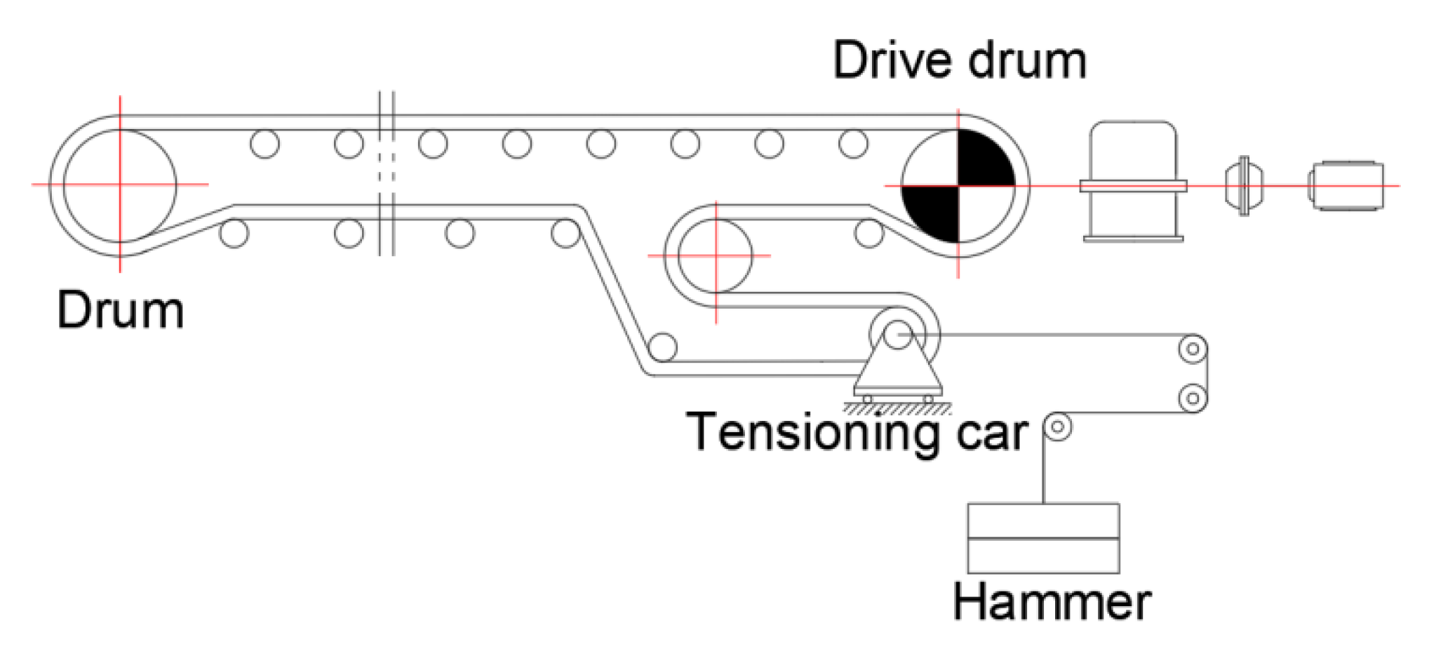
The arrangement of the conveyor is as follows (Figure 6):
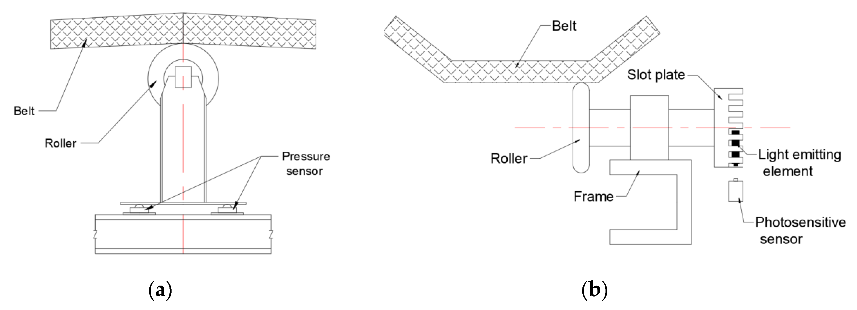
Since the sensor cannot be installed in the belt, the indirect test method is adopted. Two pressure sensors with a range of 3 tons are installed under the upper roller about 10 m away from the machine head, as shown in Figure 7a. The height of the sensor is about 5 cm, and the dynamic tension in the cross section of the belt can be calculated by recording the signal of the pressure sensor. It can be calculated by formula Fd = 2Fc/sinθ, where Fd is the dynamic tension in the cross section of the belt, Fc is the output pressure value of a single pressure sensor, and θ is the angle between the belt pushed up by the idler and the horizontal plane.
The running speed of the belt is measured by rolling a friction wheel with the belt without relative sliding. A disc is installed at the other end of the friction wheel shaft to rotate synchronously with the friction wheel, as shown in Figure 7b. The outer ring of the disc is engraved with a series of slots, and 121 pulses can be output through the photodiode when the disc rotates one circle. The instantaneous velocity of the belt can be calculated by the relationship between the pulse distance and the disc diameter.

Simulation Model

The multi-body dynamics simulation model of the machine is shown in Figure 8, in which the model includes the resistance of roller squeeze [23], the friction contact between the friction pulley and the conveyor belt [24] and the running resistance [25]. The model is established through the code we developed, and a variable topology band length solution is used. First, the conveyor belt is equally divided into N belt sections, and the belt sections are connected by an SDE. The length of the belt section is based on being able to meet the contact with the pulley. The belt sections that are not in contact with the pulley are set as a group of M, and fixed constraints are applied between the belt sections to form a long belt section. Before each simulation time step is carried out, if a certain belt section may be in contact with the pulley during this step, the constraint between the long belt sections will be dynamically lifted and converted into a normal belt section. Fixed constraints are added between ordinary belt sections that are out of contact to form long belt sections. The input parameters are shown in Table 1.
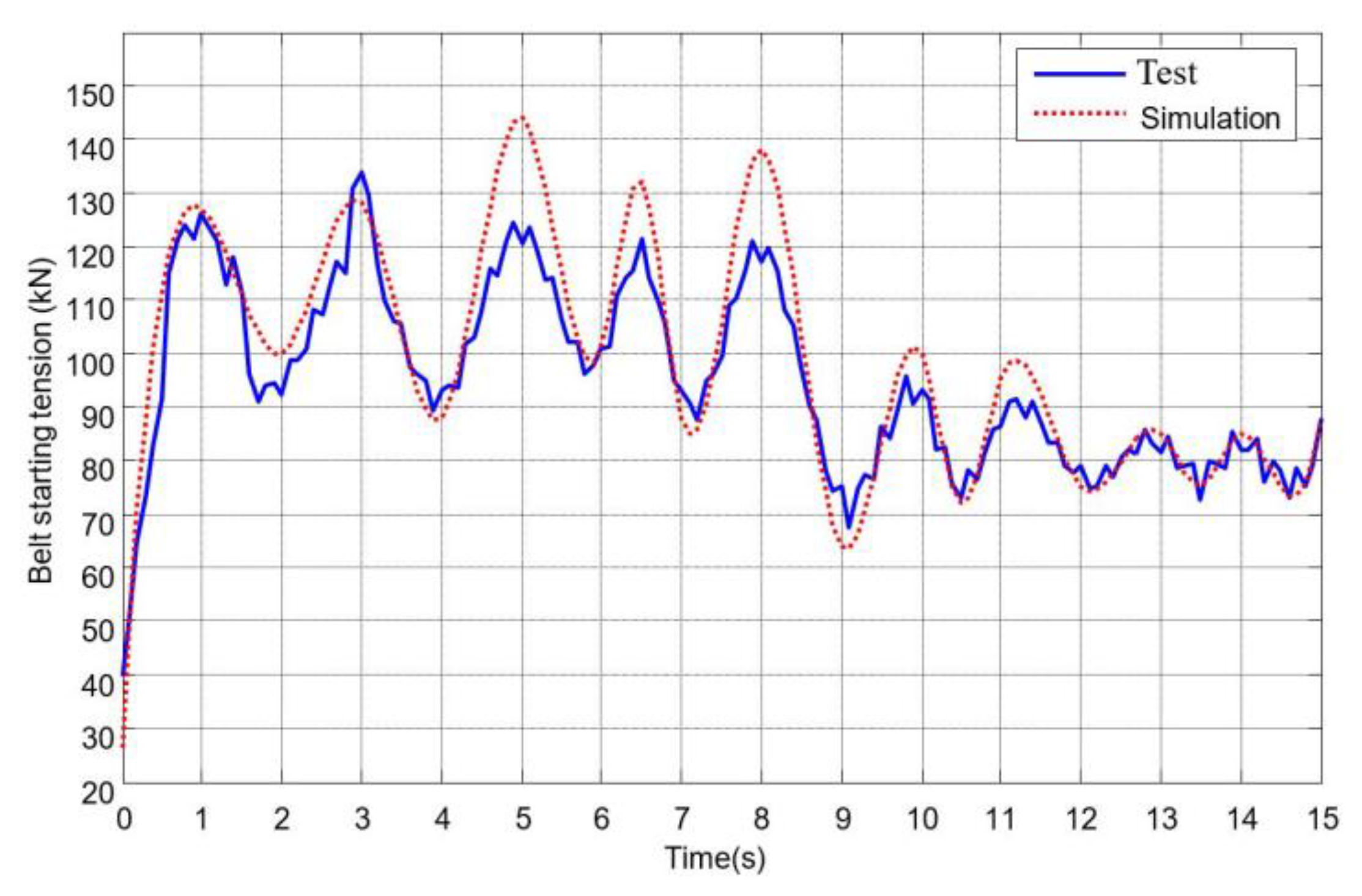
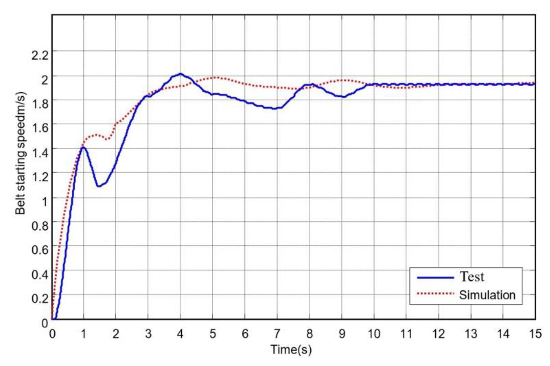
Both the measured data and the simulation results show that the peak value of dynamic tension are significantly reduced 15 s after starting, and the dynamic tension tends to be stable. Therefore, this article only makes a comparative analysis of the data within 15 s after starting.

3.2. Verification

The comparison between the simulation results and the test data is shown in Figure 9 and Figure 10. It can be seen that the changing waveforms and frequencies of the two are relatively consistent, indicating the practicality of the developed dynamic model. About 12 s after starting, the conveyor belt enters the normal working speed, and the fluctuation amplitude of the same starting tension tends to be stable. The simulation results show that the speed fluctuation of the conveyor belt is relatively gentle 0–12 s after the start of the conveyor, and the test results fluctuate obviously. This is mainly because the boundary conditions of the actual operation of the conveyor are much more complex than those given by the simulation. Overall, the dynamic analysis method of the flexible multi-body of conveyor belt is effective and accurate.

4. Discussions

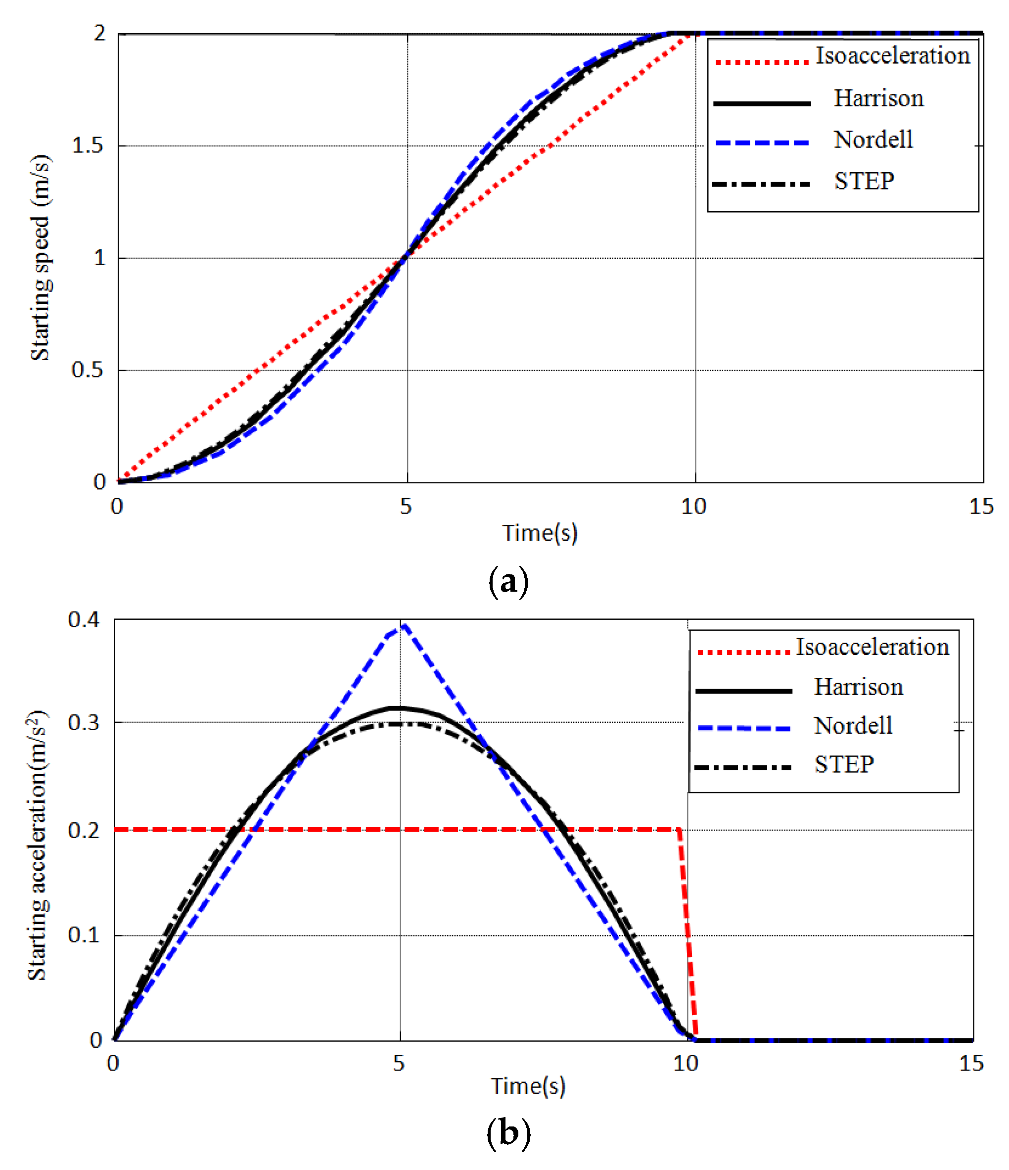
Since the dynamic tension of the belt conveyor reaches the maximum value in the starting stage, it is very important to study the factors affecting the dynamic tension in the starting process. There are many factors affecting the dynamic tension, including starting mode and time, driving mode, tension device and starting condition, etc. The ideal starting process should ensure that the acceleration curve changes gently without sudden change, and the peak value of acceleration is small. The ideal starting process should ensure that the acceleration curve changes smoothly, without abrupt changes, and the peak value of acceleration is small. US HARRISON [26] recommends the following starting speed and acceleration curve:
v ( t ) = v 0 2 ( 1 cos π t T )   0 t T
where, v0 is the initial velocity (default 0), t is the time variable, T is the total acceleration time (staring time).
Nordell [26] gives the following starting speed curve:
{ v ( t ) = 2 v 0 ( t T ) 0 t T 2 v ( t ) = 2 v 0 ( 1 + 4 t T 2 t 2 T 2 ) T 2 t T
The starting curve of Nordell is a quadratic curve. In this paper, the following cubic starting speed curve is constructed by using STEP function:
v ( t ) = v 0 ( 3 t 2 T 2 2 t 3 T 3 )     0 t T
The common starting speed curve also has the equal acceleration curve:
v ( t ) = v 0 t T     0 t T
Figure 11 shows the speed and acceleration curves of four starting modes with 10 s starting time, and all of them reach the required speed of 2 m/s after the starting time is over.
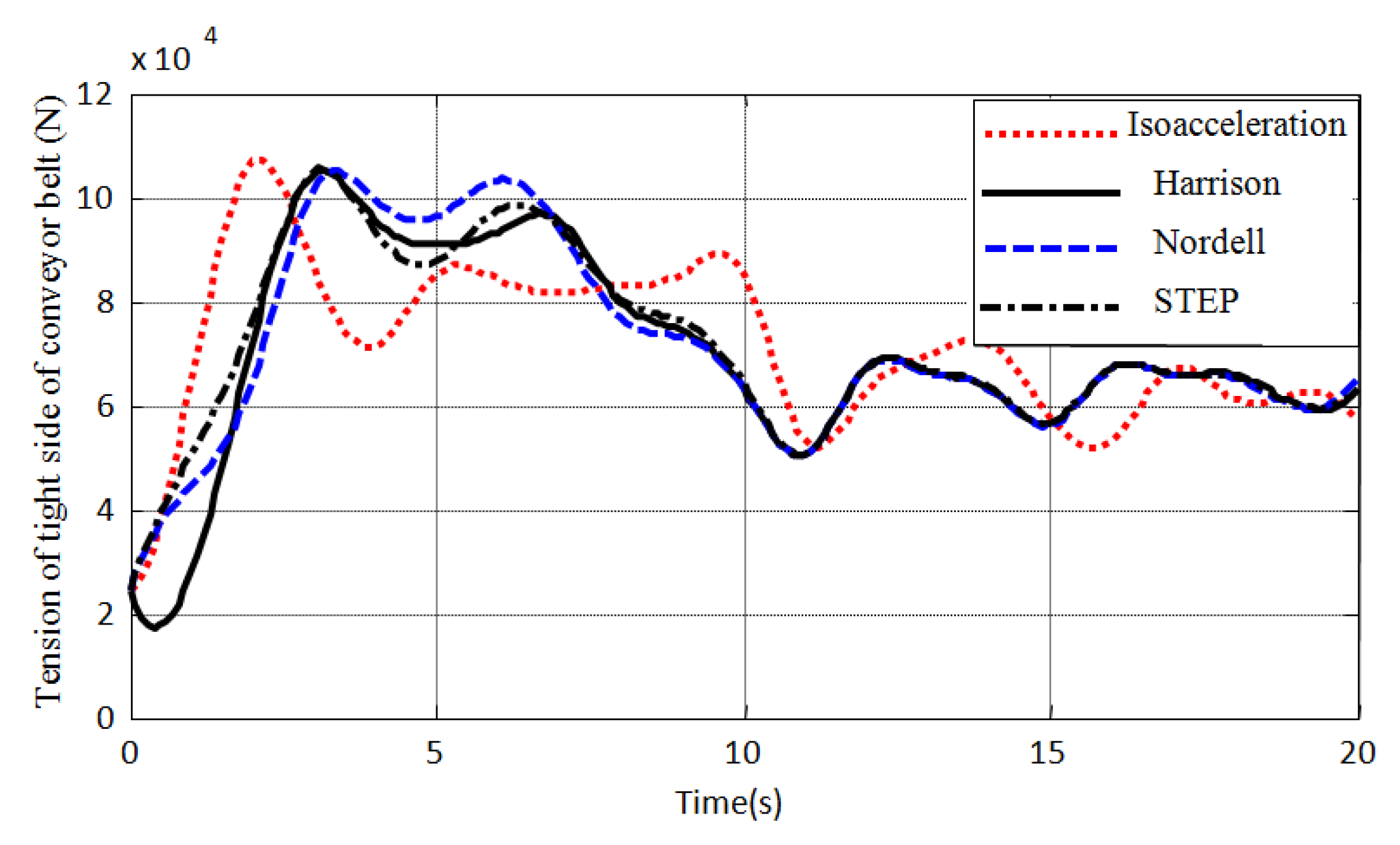
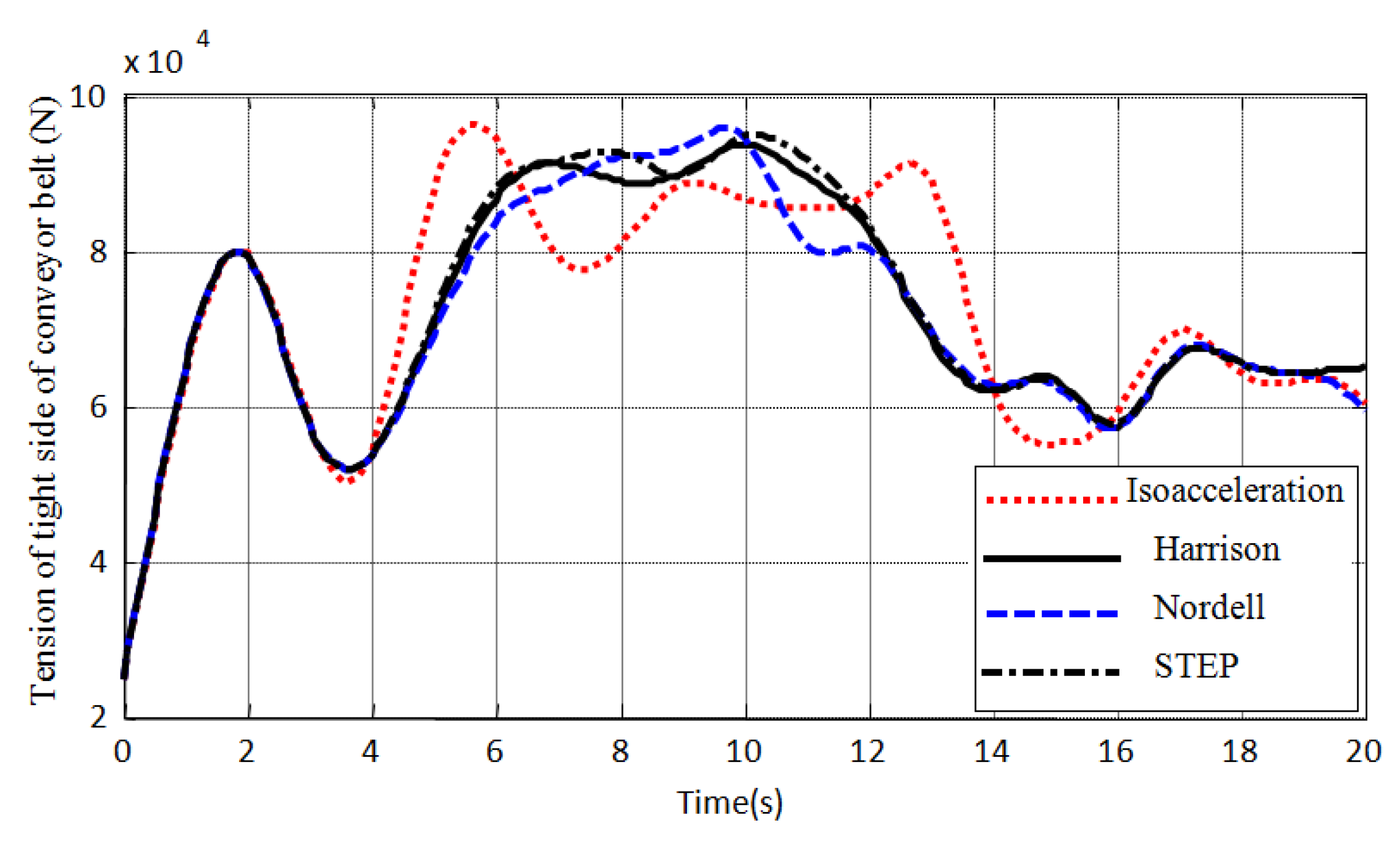
Figure 12 shows the tension on the tight side of the conveyor belt near the drive drum calculated by the model. It can be seen that: the tension amplitude of the four starting modes tends to be the same. Due to the maximum instantaneous acceleration, the maximum tension of isoacceleration start appears earliest. The amplitude of tension fluctuation is the largest, but the maximum acceleration is the smallest. Therefore, in the case of short starting time, the maximum tension value is not different from the other three curves. The other three curves have little difference, among which Nordell curve has the largest maximum tension value and the smallest fluctuation.
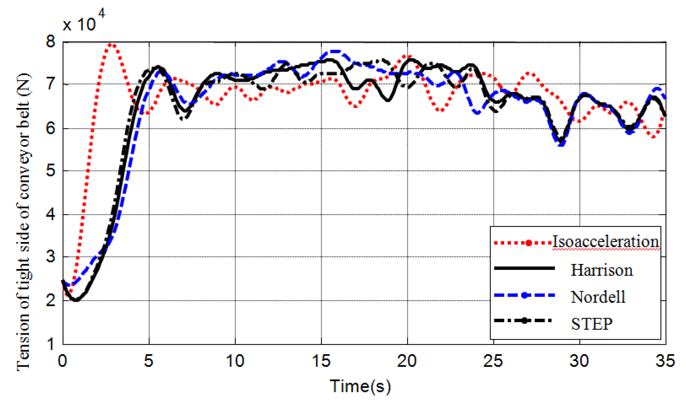
The simulation results show that reasonable increase of starting time can reduce the acceleration peak value, thus effectively reducing the starting tension of the conveyor belt. Therefore, the true starting time is increased from 10 s to 30 s. Figure 13 shows the belt tension curve with a starting time of 30 s. It can be seen that when the peak acceleration decreases, the maximum starting tension of conveyor belt decreases from 110 kN to less than 80 kN, and the fluctuation amplitude of tension also decreases obviously. The overall shape of tension curve of 10 s and 30 s starting modes is basically consistent. It shows that for the large belt conveyor, there should be enough long starting time to ensure a small dynamic tension when starting.
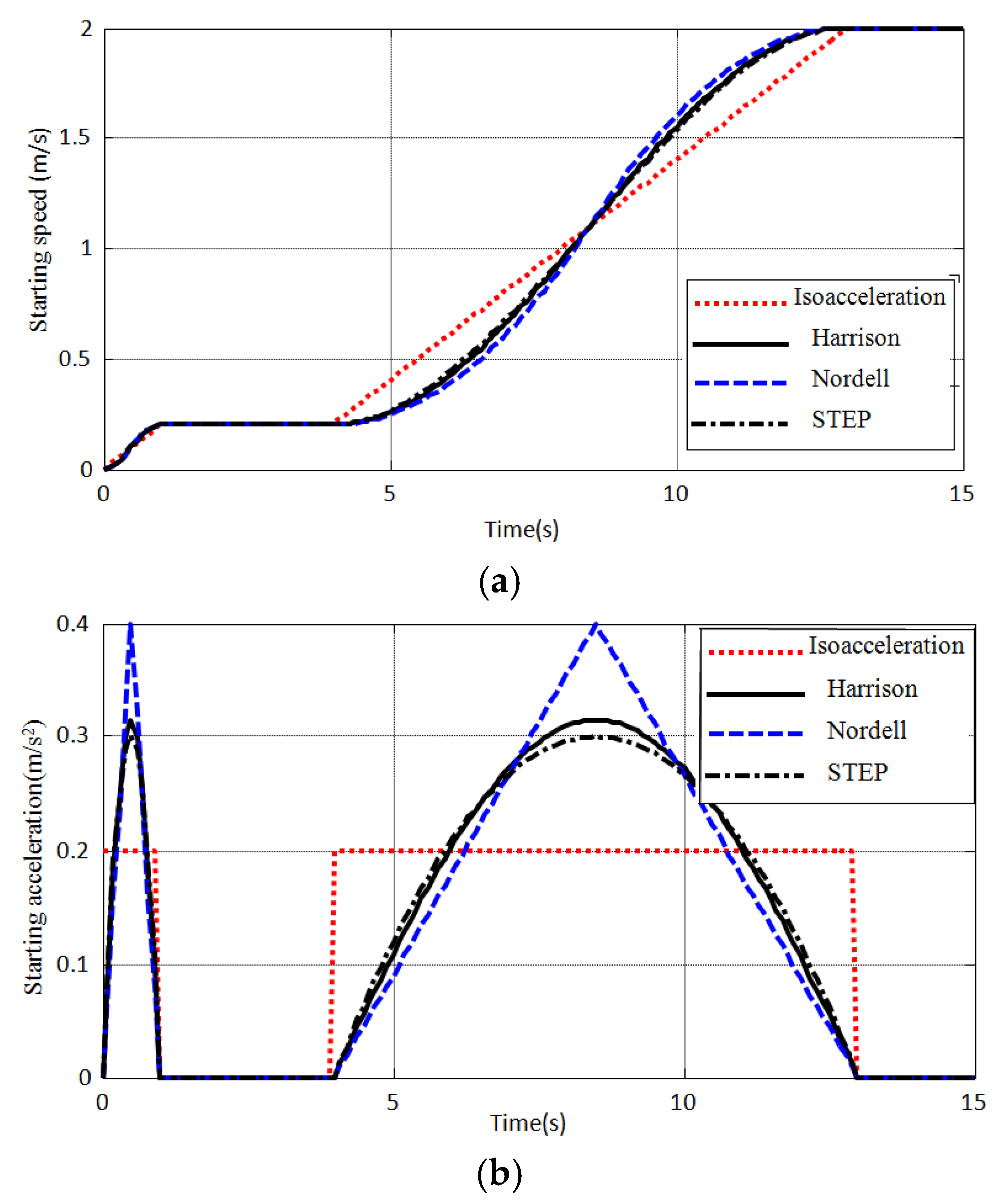
Among the four starting curves, the tension of Harrison curve is the most ideal. The tension of STEP function curve is similar to it. Due to the belt sagging in static state, a delay of about 3~8 s is often added in the initial starting stage of large belt conveyor. Thus, the conveyor belt can be tensioned before the acceleration and torque increase. Each component can enter the running state at a lower speed, further reducing the peak value of starting tension and increasing the running stability. Such a starting mode is also called pre starting. In order to study the influence of pre starting on the dynamic characteristics of belt conveyor, this paper adds a 3 s delay section in four starting speed curves with 10 s starting time. Figure 14 shows the corresponding speed and acceleration curves.
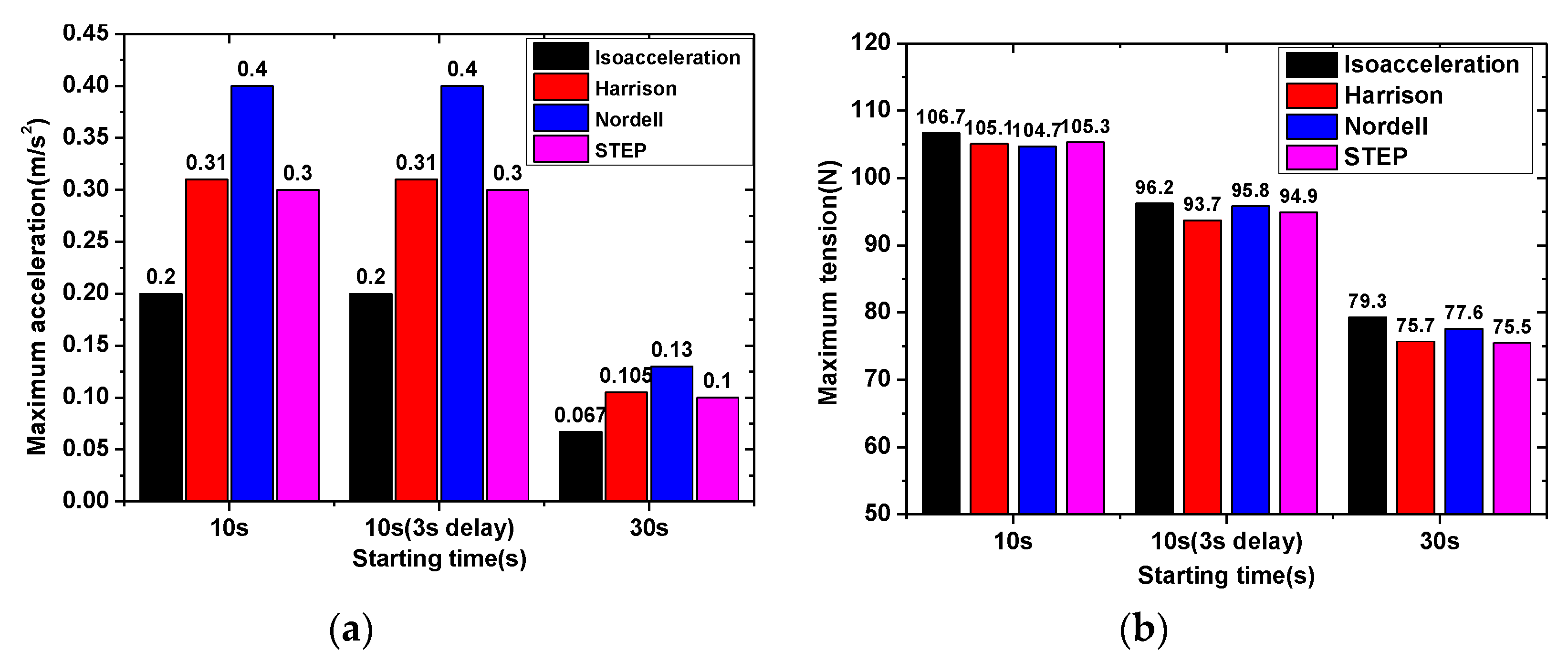
It can be seen from Figure 15 that, when starting without delay for 10 s, the tension continuously rises to the maximum value within 2~3.5 s, and then oscillates down and tends to be stable. When the starting time is 10 s and the delay is 10 s, the tension begins to decrease gradually when it reaches 80 kN in about 2 s. After the delay is over, it rises slowly again until it reaches the maximum value, and then oscillates down and tends to be stable. No matter what starting mode, the maximum tension is about 95 kN after pre-starting, which is less than 105 kN without delay starting.
It can be seen from Figure 16 that under the acceleration time of 30 s, the acceleration extremum under various starting modes is reduced by more than half. However, an acceleration time that is too long is not conducive to the improvement of transportation efficiency. Pre-start has little effect on acceleration, but can significantly reduce the extreme tension of a conveyor belt. The step function curve proposed in this paper obtains relatively low values, both in acceleration and tension.
From the discussion of parametric response of acceleration and tension, it can be concluded that: large belt conveyor should have enough long starting time to ensure small enough starting acceleration. The reasonable starting curve should meet the characteristics of minimum starting acceleration extreme value, gentle change of acceleration curve and no sudden change. It is an effective way to reduce tension extremum and fluctuation by adding delay sections to the start curve of a large belt conveyor and adopting step function curve starting.

5. Conclusions

The problems associated with the dynamic modelling of belt systems with tree system topological configurations is by the classical rigid finite body element method. The number of generalized coordinates of an open-loop system is equal to the degree of freedom of the system, so the number of system equations is the smallest. The results of dynamic simulation analysis were verified by field test. It proves the correctness of the rigid-flexible multi-body dynamic model and analysis method of the belt conveyor established in this paper.
Acceleration and tension are important evaluation indices of conveyor running stability and safety. How to get a smaller acceleration and tension on the basis of ensuring the transportation efficiency is the design optimization goal of the belt conveyor. Compared with the previous research, the method in this paper is more systematic and universal, and can easily apply belt attributes, idler attributes, collision attributes and preload attributes. It provides a theoretical basis for the optimization design of conveyor.

Author Contributions

Conceptualization, F.W. and Y.G.; methodology, F.W.; software, Y.G.; validation, F.W.; investigation, F.W.; resources, F.W.; data curation, Y.G.; writing—original draft preparation, Y.G.; writing—review and editing, Y.G. All authors have read and agreed to the published version of the manuscript.

Funding

This research was funded by the National Natural Science Foundation of China, grant number 51905237 and the Natural Science Foundation of Jiangsu Province, grant number BK20191000 and the Natural Science Foundation of Jiangsu Normal University, grant No. 18XLRX005.

Conflicts of Interest

The authors declare no conflict of interest.

Appendix A

In Equation (41):
A ˜ j , k ( p ) = ( a ˜ n j 1 + l , n k 1 + s p ) l = 1 , , n ˜ j s = 1 , , n ˜ k ,     j , k = 1 , , p ;
Q ˜ j ( p ) = ( Q ˜ n j 1 + l p ( P ˜ ( p ) ) + Q ˜ n j 1 + l p ( M ˜ ( p ) ) ) l = 1 , , n ˜ j ,     j = 1 , , p ;
e ˜ j ( p ) = ( e ˜ n j 1 + l p ) l = 1 , , n ˜ j ,     j = 1 , , p ;
g ˜ j ( p ) = ( g ˜ n j 1 + l p ) l = 1 , , n ˜ j ,     j = 1 , , p ;
a ˜ k , j ( p ) = t r ( B k ( p ) H ( p ) B j ( p ) T ) ;
e ˜ k ( p ) = t r { B k ( p ) H ( p ) [ B ˙ r B ( p ) + 2 B ˙ r B ˙ ( p ) + i = 1 n p j = 1 n p B i , j ( p ) q ˙ i ( p ) q ˙ j ( p ) ] T } ;
B k ( p ) = B ( p ) q k ( p ) = B r B ( p ) q k ( p ) ;
B k , j ( p ) = B k ( p ) q j ( p ) = B r 2 B ( p ) q k ( p ) q j ( p ) = B k , j ( p ) ;
g ˜ j ( p ) = V ˜ g ( p ) q j ( p ) ,     j = 1 , , p .
In Equation (50):
A p 1 , p 1 ( p ) = i = 1 m p A ¯ p 1 , p 1 ( p , i ) ,   A p 1 , ( p , 1 ) ( p ) = A ( p , 1 ) , p 1 ( p ) T = i = 1 m p A ¯ p 1 , ( p , 1 ) ( p , i ) ;
A p 1 , p ( p ) = A p , p 1 ( p ) T = [ A ¯ p 1 , ( p , 1 ) ( p , 2 ) A ¯ p 1 , ( p , 1 ) ( p , m p ) ] ;
A ( p , 1 ) , ( p , 1 ) ( p ) = i = 1 m p A ¯ ( p , 1 ) , ( p , 1 ) ( p , i ) ,   A ( p , 1 ) , p ( p ) = A p , ( p , 1 ) ( p ) T = [ A ¯ ( p , 1 ) , ( p , 2 ) ( p , 2 ) A ¯ p ( p , 1 ) , ( p , m p ) ( p , m p ) ] ;
A p , p ( p ) = [ A ¯ ( p , 2 ) , ( p , 2 ) ( p , 2 ) 0 0 0 0 A ¯ ( p , 2 ) , ( p , 2 ) ( p , 2 ) 0 0 0 0 A ¯ ( p , i ) , ( p , i ) ( p , i ) 0 0 0 0 A ¯ p ( p , m p ) , ( p , m p ) ( p , m p ) ] ;
Q p 1 ( p ) = i = 1 m p Q ¯ p 1 ( p , i ) ,   Q ( p , 1 ) ( p ) = i = 1 m p Q ¯ ( p , 1 ) ( p , i ) ;
Q p ( p ) = [ Q ¯ ( p , 2 ) ( p , 2 ) Q ¯ ( p , 3 ) ( p , 3 ) Q ¯ ( p , i ) ( p , i ) Q ¯ ( p , m p ) ( p , m p ) ] T ;
e p 1 ( p ) = i = 1 m p e ¯ p 1 ( p , i ) ,   e ( p , 1 ) ( p ) = i = 1 m p e ¯ ( p , 1 ) ( p , i ) ,   e p ( p ) = [ e ¯ ( p , 2 ) ( p , 2 ) e ¯ ( p , 3 ) ( p , 3 ) e ¯ ( p , i ) ( p , i ) e ¯ ( p , m p ) ( p , m p ) ] T ;
g p 1 ( p ) = i = 1 m p g ¯ p 1 ( p , i ) ,   g ( p , 1 ) ( p ) = i = 1 m p g ¯ ( p , 1 ) ( p , i ) ;
g p ( p ) = [ g ¯ ( p , 2 ) ( p , 2 ) g ¯ ( p , 3 ) ( p , 3 ) g ¯ ( p , i ) ( p , i ) g ¯ ( p , m p ) ( p , m p ) ] T .
In Equation (51):
A ( p ) = [ A ( p 1 ) + A p 1 , p 1 ( p ) A p 1 , ( p , 1 ) ( p ) A p 1 , p ( p ) A ( p , 1 ) , p 1 ( p ) A ( p , 1 ) , ( p , 1 ) ( p ) A ( p , 1 ) , p ( p ) A p , p 1 ( p ) A p , ( p , 1 ) ( p ) A p , p ( p ) ] ;
Q ( p ) = [ Q ( p 1 ) + Q p 1 ( p ) Q ( p , 1 ) ( p ) Q p ( p ) ] ,   e ( p ) = [ e ( p 1 ) + e p 1 ( p ) e ( p , 1 ) ( p ) e p ( p ) ] ,   g ( p ) = [ g ( p 1 ) + g p 1 ( p ) g ( p , 1 ) ( p ) g p ( p ) ] ;
v ( p ) = [ 0 0 v p ( p ) ] ,   w ( p ) = [ 0 0 w p ( p ) ] .

References

  1. Bajda, M.; Blazej, R.; Jurdziak, L. Analysis of changes in the length of belt sections and the number of splices in the belt loops on conveyors in an underground mine. Eng. Fail. Anal. 2019, 101, 436–446. [Google Scholar] [CrossRef]
  2. Fan, J.; Liu, T.; Chen, S. Analysis of dynamical behaviors of a 2-DOF friction-induced oscillator with one-sided impact on a conveyor belt. Nonlinear Dyn. 2019, 97, 797–830. [Google Scholar] [CrossRef]
  3. Feng, Y.; Zhang, M.; Li, G.; Meng, G. Dynamic characteristic analysis and startup optimization design of an intermediate drive belt conveyor with non-uniform load. Sci. Prog. 2019, 103, 39951860. [Google Scholar] [CrossRef] [PubMed] [Green Version]
  4. Yang, C.H.; Mao, J.; Li, C.L. Study of indentation resistance of conveyor belt. J. China Coal Soc. 2010, 35, 149–153. [Google Scholar]
  5. Czaplicka, K. Analysis of stress relaxation processes in conveyor belts. Mech. Compos. Mater. 1994, 30, 411–415. [Google Scholar] [CrossRef]
  6. Li, W.; Xin, Z. Flexural fatigue life prediction of a tooth V-belt made of fiber reinforced rubber. Int. J. Fatigue 2018, 111, 269–277. [Google Scholar] [CrossRef]
  7. Li, G.; Li, R. Belt Conveyor modeling and performance simulation based on AMESim. In Proceedings of the 2009 Second International Conference on Information and Computing Science, Manchester, UK, 21–22 May 2009. [Google Scholar]
  8. Kulinowski, P. Analytical method of designing and selecting take-up systems for mining belt conveyors. Arch. Min. Sci. 2013, 58, 1301–1315. [Google Scholar]
  9. Kulinowski, P. Simulation method of designing and selecting tensioning systems for mining belt conveyors. Arch. Min. Sci. 2014, 59, 123–138. [Google Scholar] [CrossRef]
  10. Schulz, G. Comparison of drives for long belt conveyors. Bulk Solids Handl. 1995, 15, 247–251. [Google Scholar]
  11. Carretero, L.; Valero, J. Existence of periodic solutions for a scalar differential equation modelling optical conveyor belts. J. Math. Anal. Appl. 2019, 480, 123385. [Google Scholar] [CrossRef]
  12. Lu, Y.; Li, Q. A regression model for prediction of idler rotational resistance on belt conveyor. Meas. Control 2019, 52, 441–448. [Google Scholar] [CrossRef]
  13. Munzenberger, P.J.; OShea, J.I.; Wheeler, C.A. A comparison of rubber stress relaxation models for conveyor belt indentation rolling resistance calculations. Int. J. Mech. Mater. Des. 2019, 15, 213–224. [Google Scholar] [CrossRef]
  14. Li, J.; Pang, X. Belt Conveyor Dynamic Characteristics and Influential Factors. Shock Vib. 2018, 8106879. Available online: https://doi.org/10.1155/2018/8106879 (accessed on 12 August 2020).
  15. Suweken, G.; Van Horssen, W.T. On the transversal vibrations of a conveyor belt with a low and time-varying velocity. Part II: The beam-like case. J. Sound Vib. 2003, 267, 1007–1027. [Google Scholar] [CrossRef]
  16. Shen, J.; Wheeler, C.; O’Shea, J.; Ilic, D. Investigation of the dynamic deflection of conveyor belts via experimental and modelling methods. Measurement 2018, 127, 210–220. [Google Scholar] [CrossRef]
  17. Ilic, D.; Wheeler, C. Measurement and simulation of the bulk solid load on a conveyor belt during transportation. Powder Technol. 2017, 307, 190–202. [Google Scholar] [CrossRef]
  18. Woźniak, D. Laboratory tests of indentation rolling resistance of conveyor belts. Measurement 2020, 150, 107065. [Google Scholar] [CrossRef]
  19. Wittbrodt, E.; Adamiec-Wójcik, I.; Wojciech, S. Dynamics of Flexible Multibody Systems; Springer: Berlin/Heidelberg, Germany, 2006. [Google Scholar]
  20. Hou, Y.F.; Meng, Q.R. Dynamic characteristics of conveyor belts. J. China Univ. Min. Technol. 2008, 18, 629–633. [Google Scholar] [CrossRef]
  21. Gaull, A. A rigorous proof for the equivalence of the projective Newton–Euler equations and the Lagrange equations of second kind for spatial rigid multibody systems. Multibody Syst. Dyn. 2019, 45, 87–103. [Google Scholar] [CrossRef]
  22. Wang, F.S. Research on flexible multibody dynamics modeling of conveyor belt. Mech. Transm. 2018, 042, 43–46. [Google Scholar]
  23. Wang, F.S.; Jiang, H.Q. Analysis for boundary element of sag resistance of belt conveyer. Hoisting Conveying Mach. 2014, 45, 97–100. [Google Scholar]
  24. Wang, F.S.; Hou, Y.F. Analysis on contact problem of rigid cylinder with viscoelastic foundation. J. Mach. Des. 2010, 27, 15–17. [Google Scholar]
  25. Hunter, S.C. The rolling contact of a rigid cylinder with a viscoelastic half space. J. Appl. Mech. 1961, 28, 611. [Google Scholar] [CrossRef]
  26. Mao, J.; Shi, J.G.; Zhang, D.S. Starting characteristics and controllable starting technology of belt conveyor. Min. Process. Equip. 2004, 2, 19–22. [Google Scholar]
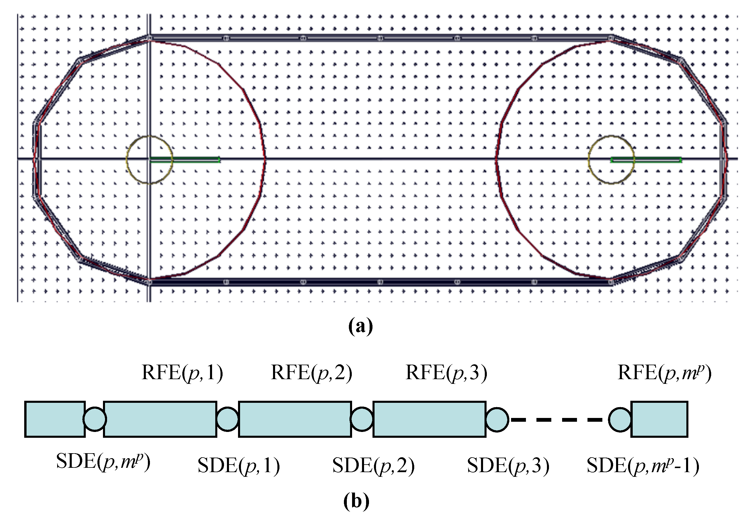
Figure 1. Discrete model of the belt. (a) rigid finite belt model; (b) element composition.
Symmetry 12 01489 g001
Figure 2. Coordinate system of a rigid finite element i.
Symmetry 12 01489 g002
Figure 3. Coordinate system of the spring damping element (SDE) j.
Symmetry 12 01489 g003
Figure 4. Deformation of SDE j.
Symmetry 12 01489 g004
Figure 5. Coordinate system of rigid bodies.
Symmetry 12 01489 g005
Figure 6. Measured layout of belt conveyor.
Symmetry 12 01489 g006
Figure 7. Measured layout of belt conveyor: (a) Principle of roller pressure test; (b) Principle of speed measurement.
Symmetry 12 01489 g007
Figure 8. Simulation model of belt conveyor.
Symmetry 12 01489 g008
Figure 9. Starting tension of conveyor belt.
Symmetry 12 01489 g009
Figure 10. Starting speed of conveyor belt.
Symmetry 12 01489 g010
Figure 11. Starting mode (staring time 10 s) (a) speed; (b) acceleration.
Symmetry 12 01489 g011
Figure 12. Conveyor belt tension under different starting speed (starting time 10 s).
Symmetry 12 01489 g012
Figure 13. Conveyor belt tension under different starting speed (starting time 30 s).
Symmetry 12 01489 g013
Figure 14. Acceleration under different starting speed (adding delay section). (a) speed; (b) acceleration.
Symmetry 12 01489 g014
Figure 15. Conveyor belt tension under different starting speed (adding delay section).
Symmetry 12 01489 g015
Figure 16. Comparison of different starting mode. (a) acceleration; (b) tension.
Symmetry 12 01489 g016
Table 1. Belt conveyor parameters.
Performance parameterTransportation distance: 972 m
Transportation capacity: 400 t/h
Belt speed: 2 m/s
Driving deviceRated power of motor: 150 KW
Rated speed: 1000 rpm
Diameter of driving drum: 0.8 m
Drum mass: 800 kg
Conveyor beltTensile strength: 1250 N/m
Belt width: 1 m
Mass per unit length of conveyor belt: 24.5 kg/m
Conveying materials56 kg/m
Model parameters and running resistanceLength of belt section: 314.23 mm
Number of belt sections: 170
System degree of freedom: 309