Computational Costs of Multi-Frontal Direct Solvers with Analysis-Suitable T-Splines

Abstract

In this paper, we consider the computational cost of a multi-frontal direct solver used for the factorization of matrices resulting from a discretization of isogeometric analysis with T-splines, and analysis-suitable T-splines. We start from model projection or model heat transfer problems discretized over two-dimensional meshes, either uniformly refined or refined towards a point or an edge. These grids preserve several symmetries and they are the building blocks of more complicated grids constructed during adaptive isotropic refinement procedures. A large class of computational problems construct meshes refined towards point or edge singularities. We propose an ordering that permutes the matrix in a way that the computational cost of a multi-frontal solver executed on adaptive grids is linear. We show that analysis-suitable T-splines with our ordering, besides having other well-known advantages, also significantly reduce the computational cost of factorization with the multi-frontal direct solver. Namely, the factorization with N T-splines of order p over meshes refined to a point has a linear O(Np⁴) cost, and the factorization with T-splines on meshes refined to an edge has O(N2^pp²) cost. We compare the execution time of the multi-frontal solver with our ordering to the Approximate Minimum Degree (AMD) and Cuthill–McKee orderings available in Octave.

1. Introduction

Higher-order and continuity basis functions, such as B-splines, Non-Uniform Rational B-splines (NURBS) [1], and T-splines [2], are used in computer-aided design (CAD)/computer-aided engineering (CAE) systems for modeling of the geometry of engineering design. The idea of the isogeometric analysis (IGA) [1] is to use such higher-order and continuity basis functions for solving different engineering problems with the finite element method. Besides B-splines, NURBS, and T-splines, some other families of functions were introduced recently in the context of IGA [3,4,5,6,7,8,9,10].

Multi-frontal solvers are popular tools for the factorization of sparse matrices [11,12,13]. The advantage of multi-frontal solvers is that they provide an accurate numerical solution for any computational problem, symmetric, unsymmetric, positive definite, non-positive definite, double precision, or complex. The price to pay is the computational cost, usually higher than that for iterative solvers.

This computational cost in the context of isogeometric analysis with higher-order B-spline basis functions has been analyzed in [14], and in the context of B-splines with C⁰ separators, which are equivalent to Lagrange polynomials, in [15]. The B-spline basis functions are defined over regular patches of elements, and the computational cost of factorization for a mesh with N B-spline basis functions of order p can be estimated as O(N²) for B-splines with C⁰ continuity [15] and as O(N²p³) for B-splines with C^p−1 continuity for three-dimensional grids [14]. It has also been shown in [16] that local reduction in B-spline continuity on uniform grids allows reducing the constant in front of the computational cost.

However, these results refer to the uniform patch of elements, and the computational cost of the multi-frontal solver of IGA on adaptive grids has not been analyzed so far. For extension of IGA into a non-uniform adaptive grid, we need to move from B-spline basis functions to one of their extensions. We selected the T-spline basis functions [2] since they are most popular for adaptive computations with higher-order and continuity basis functions. Still, there are several other options for discretization available [3,4,5,6,7,8,9,10], and we may analyze the computational costs of these alternative basis functions in possible future work.

The standard finite element method uses the basis functions of C⁰ continuity, and the computational costs of the multi-frontal solver for adaptive grids with standard FEM have been analyzed in [15]. In this paper, for the first time, we will analyze the computational cost of multi-frontal solvers applied to isogeometric analysis with T-spline basis functions on adaptive grids.

Multi-frontal solvers construct orderings and elimination trees based on a matrix’s sparsity pattern resulting from discretization over the computational mesh. They utilize different algorithms for the construction of the orderings. There are several possible ordering algorithms focused on analyzing of the sparsity pattern of the matrix (e.g., Approximate Minimum Degree (AMD) [17], Paderborn ORDering tools (PORD) [18], and nested dissections [19]). It has been shown that the nested dissection algorithm is optimal for computations with uniform grids [20]. There are also some ordering algorithms analyzing the structure of the computational mesh [21,22,23,24] instead of the structure of the sparse matrix.

This paper focuses on the T-spline basis functions, which can be defined on adaptive grids.

We start from recalling the definition of B-spline basis functions, where B_i,0(x) = 1 for x in [x_i,x_i+1], and B_i,p(x) = (x − x_i)/(x_i+p − x_i)B_i,p−1(x) + (x_i+p+1 − x)/(x_i+p+1 − x_i+1)B_i+1,p−1(x) for x in [x_i,x_i+p+1]. If the knot points are repeated in the denominator, this term is cancelled (since division by zero is not allowed). The B-splines of order p span over p + 1 elements and they are defined with p + 2 knot points, which are introduced into the recursive formula for B-spline basis functions. Thus, the B-spline basis in 1D is defined with a knot vector, e.g., [0 0 1 2 2] defines linear C⁰ B-splines, [0 0 0 1 2 2 2] defines quadratic C¹ B-splines, and [0 0 0 1 1 2 2 2] defines quadratic C⁰ B-splines.

Let us follow the state-of-the-art process of constructing the sparse matrix, ordering, and the elimination tree for an exemplary two-dimensional mesh with C⁰ B-spline basis functions. The B-spline basis functions are usually defined with a tensor product of one dimensional B-splines B_ij;p(x,y) = B_i;p(x)B_j,p(y), described by knot vectors [1]. The basis functions obtained by a tensor product of the 1D B-splines defined by knot vectors [0 0 0 1 1 2 2 2] and [0 0 0 1 1 2 2 2] are presented in Figure 1.

We enumerate the B-spline basis functions from 1 to 25, since we have five one-dimensional B-splines in each direction, and the tensor product results in 5⋅5 = 25 basis functions. We construct a matrix (see Figure 2) where rows and columns correspond to the B-splines, and the non-zero values represent overlaps of spans of the B-splines. The particular values depend on the problem being discretized with B-splines over the computational mesh—e.g., the projection problem involves integrals with the multiplications of the pairs of B-splines ∫B_i;p(x)B_j,p(y)B_k;p(x)B_l,p(y)dxdy, and the heat transfer problem involves integrals with the multiplications of the gradients of the pairs B-splines ∫∇(B_i;p(x)B_j,p(y))°∇(B_k;p(x)B_l,p(y))dxdy.

The nested dissections ordering algorithm [19] constructs the elimination graph (see Figure 2) representing the matrix’s sparsity pattern. The nodes in the graph represent the B-spline basis functions. They also represent the rows in the matrix. The edges represent the overlaps of the B-splines and the non-zero values in the columns of the matrix.

To describe this state-of-the-art nested dissection algorithm, we need to recall the Breadth-First Search (BFS) algorithm and introduce the concept of a separator and a peripheral node.

The Breadth-First Search algorithm (BFS) is used for visiting nodes of the graph; it starts at some arbitrary node of a graph and explores the neighboring nodes first before moving to the next layer of neighbors. The execution of the BFS algorithm can identify levels with a group of nodes. In the example presented in Figure 2, the BFS algorithm was executed from node 23, and it has found three levels: the first level with node 23, the second level with all the neighbors of node 23, and the third level with all neighbors of the nodes from the second level, which were not visited before.

A separator it is a set of nodes from the middle level having neighbors from the next level. In this example, the separator consists of nodes 11,12,13,14, and 15.

A peripheral node is a node with a higher number of levels obtained from the BFS algorithm’s execution, starting from this node, and the shortest separator resulting from execution of the BFS algorithm (starting from this node). In the example presented in Figure 2, it is node 23 (but some other boundary nodes may also qualify, e.g., 3,11, or 15).

The nested dissections algorithm recursively finds separators. It first finds a peripheral node and a separator; then, it partitions the graph into two subgraphs according to the separator and it finds new separators for subgraphs in a recursive way. This is illustrated in Figure 3.

On the base of graph partition and separators, the elimination tree can be identified by listing the separators in a tree structure (see Figure 3). The elimination of unknowns is then performed in a multi-frontal manner. The rows are eliminated in the order resulting from browsing of the elimination tree from leaves up to the root. In our example, the order of elimination is:

• 1,2,6,7, which can be performed on a local sub-matrix of the global sparse matrix, called the frontal matrix. These rows represent B-splines that overlap with B-splines 3,8,11,12, and 13. Thus, this frontal matrix has a size of nine (with rows 1,2,6,7,3,8,11,12, and 13), and this step eliminates four rows (1,2,6, and 7).
• 4,5,9,10, which can be performed on another frontal matrix, and these B-splines overlap with 3,8,13,14, and 15. This frontal matrix has a size of nine (with rows 4,5,9,10,3,8,13,14, and 15), and this step eliminates four rows (4,5,9, and 10).
• 16,17,21,22 (the third frontal matrix); they overlap with 18, 23, and 11,12, and 13. This frontal matrix has, again, a size of nine (with rows 16,17,21,22,18,23,11,12, and 13), and this step eliminates four rows (16,17,21, and 22).
• 19,20,24,25 (the fourth frontal matrix); they overlap with 18,23,13,14, and 15. This frontal matrix, as with the previous ones, has a size of nine (with rows 19,20,24,25,18,23,13,14, and 15), and this step eliminates four rows (19,20,24, and 25).

In the next level, we merge the frontal matrices according to the structure of the elimination tree and we perform further eliminations:

• Merge the first and the second frontal matrices into a fifth frontal matrix, and eliminate rows 3 and 8. This time, the frontal matrix has a size of seven (it contains rows 3,8,11,12,13,14, and 15) and this step eliminates two rows (3 and 8).
• Merge the third and fourth frontal matrices into a sixth frontal matrix and eliminate rows 18 and 23. This time, the frontal matrix has a size of seven (it contains rows 18,23,11,12,13,14, and 15) and this step eliminates two rows (18 and 23).
• Merge the fifth and the sixth frontal matrices and eliminate all the rows. This frontal matrix has a size of five (it contains rows 11,12,13,14, and 15) and this step eliminates all the rows.

This procedure is implemented in multi-frontal solvers, e.g., those available through the PETSc interface [25], such as MUMPS solver [11,12,13], Scalapack [26], PaStiX [27], and SuperLU [28]. To find the computational cost of the elimination process, we can look at the spans of B-spline basis functions and the way they overlap with other B-spline functions. We can identify the dimensions of the frontal matrices (called a) and the number of eliminated rows (B-splines basis functions, called b). The cost of elimination of b rows from the matrix of size a is O(ab²) [29]. Thus, the procedure’s total cost is Σi = 1, …, s a_ib_i², where s is the number of steps (number of layers in the elimination tree representing the separators), and we need to identify the number of steps and the dimensions of the frontal matrices and the eliminated rows.

T-spline basis functions are a generalization of B-splines into non-uniform grids. From the point of view of the multi-frontal solver’s computational cost, the exact formula of the basis functions is not important, only the support of the function. The knot vectors for T-splines span over the adaptive grids. For the simplicity of presentation, we restricted our example to even T-splines. The centers of such even T-splines are located over the center of an element. We have one knot vector span in the horizontal direction, where the knot points are located at the cross-sections with mesh edges. We also have another knot vector span in the vertical direction, defined in a similar way. We have one T-spline associated with one mesh element, where its center is located. Thus, the T-splines can be identified with mesh elements. In Figure 4, we present the T-spline span over the mesh refined towards the corner.

T-splines are usually defined over so-called analysis-suitable grids. They were proposed to deal with the approximation properties of T-splines [30], but they were not analyzed in the context of the solvers’ computational cost, which is the topic of this paper. Analysis-suitable grids are obtained by adding so-called T-junction extensions [29]. The edges that end up with hanging nodes (nodes that belong to three elements, located on the edge between two small elements and one big element) are extended into p/2 blocks, where p denotes the order of T-splines’ span over the analysis-suitable mesh. The analysis-suitable grid obtained by the extension of the grid refined towards a point and the resulting T-splines are presented in Figure 4. The T-splines spanning over the analysis-suitable mesh are called the analysis-suitable T-splines.

The structure of this paper is as follows. In Section 2, we present the motivation for this research. In Section 3, we analyze the computational cost of T-splines on uniform grids. In this case, the T-splines are equivalent to B-splines (in the sense of supports), and the analysis-suitable grid is the same as the original uniform grid. Next, in Section 4, we estimate the computational cost of T-splines on an adaptive grid, in Section 4.1 on grids refined towards a point, and in Section 4.2 on grids refined towards an edge. In the following Section 5, we estimate the computational cost of the analysis-suitable T-splines defined on grids refined towards a point, in Section 5.1. and defined on grids refined towards an edge. in Section 5.2. Section 6 is devoted to numerical verification of the proposed ordering algorithms. We conclude the paper in Section 7.

2. Motivation

The computational cost of a multi-frontal solver varies from N to N³, depending on the computational mesh’s sparsity pattern or the computational mesh structure and basis functions used for discretization. The general formula for any mesh and basis functions is not known. It has been estimated for uniform and some adaptive grids and selected basis functions.

The computational costs for the multi-frontal solver executed on uniform meshes are known for discretization with the linear finite element method (FEM) [20]. The cost has also been estimated for the finite element method with hierarchical Lagrange basis functions of order p [31] and the isogeometric finite element method with B-spline basis functions [14]. Namely, for the classical FEM on 2D uniform grids, it is O(N^1.5), and for 3D uniform grids, it is O(N²). For IGA discretization, we have an extra term related to the polynomial order, and for B-spline-based discretization with uniform grids, it is O(N² p³) for 3D grids. This cost has been not estimated for 2D grids yet. For uniform grids, the T-splines and B-splines and analysis-suitable T-splines are equivalent by definition. The computational costs for the multi-frontal solver executed on adaptive grids are known for hierarchical Lagrange polynomials for different singularities [15,32]. They are not estimated for T-spline and analysis-suitable T-spline basis functions. In [32], there is an asymptotic estimation of the computational cost for refined grids based on Lagrange polynomials. It is estimated as O(N^{max(3(q−1)/q,1)}), where q is the type of singularity, and this result does not depend on the dimension of the mesh. However, this computational cost is not known for T-spline and analysis-suitable T-spline basis functions for any kind of grids. In general, for discretizations with T-splines, we expect these costs to be higher than those for standard FEM and IGA, and for analysis-suitable T-splines, we expect them to have an extra factor related to the polynomial orders. In this paper, we derive these costs and factors. The optimization of computational cost of IGA solvers is important, since IGA has multiple applications to phase field modeling with either Cahn–Hilliard [33] or Navier–Stokes–Korteweg higher-order models [34]. The IGA-FEM has been also successfully applied for solution of non-linear problems, such as wind turbine aerodynamics [35], incompressible hyper-elasticity [36], or blood flow simulations [37].

This work’s main motivation is to derive computational costs for a multi-frontal solver executed on different grids, either uniform or refined towards a point or edge singularity, with T-spline basis functions and analysis-suitable T-spline basis functions. Based on these estimations, we propose ordering algorithms resulting in a permutation of the sparse matrix such that the computational cost of multi-frontal solver algorithm factorization is linear for grids refined towards point or edge singularities when using analysis-suitable T-splines.

Input: Mesh, p (order of analysis suitable T-splines)

Level = 1;

Nodes = nodes from the top level of the mesh;

Tree = build tree (Level, Nodes);

Output: ordering = post-order traversal of Tree;

build tree (Level, Nodes)

{

   Node = create node (Nodes);

   Level = Level + 1;

   Node -> left = build tree (Level, first p + 1 nodes from Level neighboring to Nodes);

   Node -> right = build tree (Level, last p + 1 nodes from Level neighboring to Nodes);

   return Node;

}

The algorithm constructs a binary tree with nodes assigned to elements on levels of the refinement. The root is the largest element, and the leaves are the smallest elements. It orders the elements and T-splines assigned to them by post-order traversal of the tree. For grids refined towards a point, it is equivalent to browsing the mesh layer by layer; see Figure 5.

Computational grids used in CAD/CAE systems can be partitioned into sub-grids, either uniform (without local refinements) or refined towards a point or edge singularity, or they are a composition of such refinements towards several point or edge singularities. To estimate the computational costs for all kinds of grids, we take three representative grids: the point singularity, the edge singularity, and the uniform grid. Most other grids in two dimensions are constructed by combining these three representative grids, and so are the computational costs. Our ordering algorithm can be easily combined with the domain decomposition approach of complex grids.

3. Uniform Mesh

In this section, we estimate the computational cost of the multi-frontal solver on uniform grids.

In this case, the B-splines are equivalent to T-splines and to the analysis-suitable T-splines. All these basis functions have identical supports on uniform grids. We assume that we have a uniform mesh that consists of 2^2s of blocks, each block being of size (p+ 1)(p+ 1). The number of mesh elements N is equal to (p+ 1)(p+ 1)2^2s and so is the number of T-splines. Some examples of meshes with p = 2 and 4 are presented in Figure 6. We assume even polynomial orders for the simplicity of the derivations, but our results remain valid also for odd cases. In the first step (I = 0), the multi-frontal algorithm will eliminate T-splines connected with each block’s middle element. It will generate a frontal matrix with rows and columns related to the T-splines from this particular block. Only one row representing the T-splines from the center of the block can be eliminated here, since it is the support span inside the block. We will talk about the T-splines to be eliminated for simplicity of presentation, the ones having supports inside the processed blocks, and not about the rows and matrices.

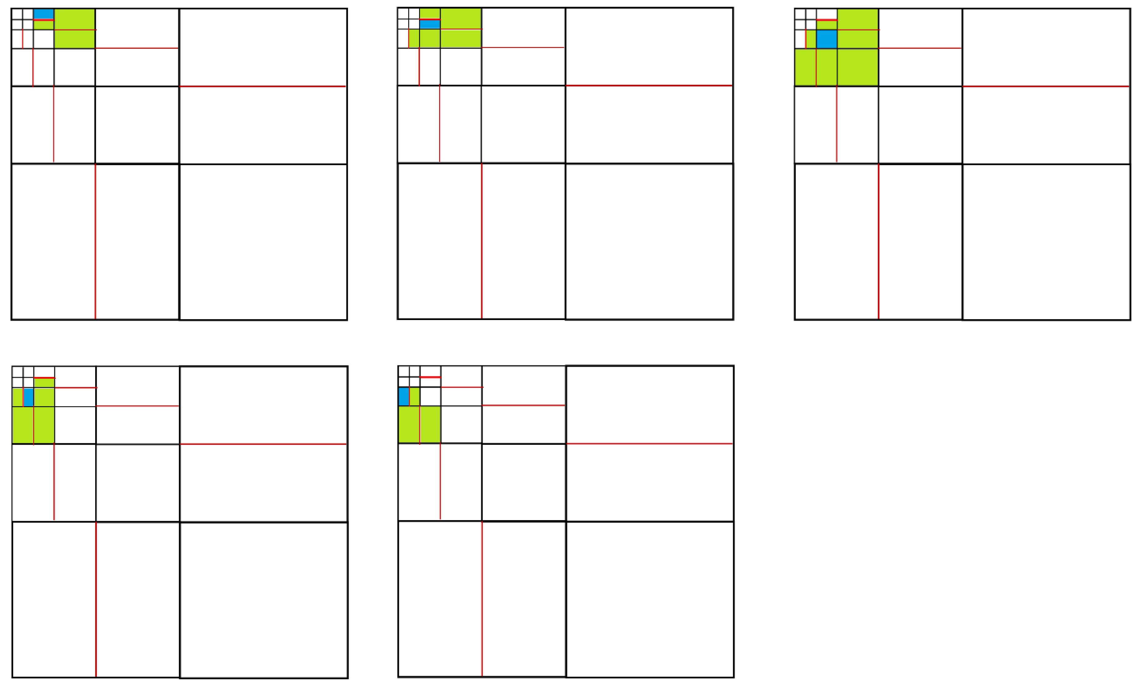
The algorithm will then join four neighboring blocks (3⋅3 for p = 2) into one bigger block and eliminate these T-splines that can be eliminated (T-splines located on the common edge, with support spans inside the two merged blocks). The algorithm will follow this pattern in the following steps: join four neighboring blocks into bigger blocks and eliminate T-splines that can be eliminated. Figure 7 and Figure 8 present, step by step (iteration step i equal to 0, 1, and 2), the elements for which the T-splines can be eliminated (green color), for which the T-splines were eliminated in previous steps (white color), and the rest of the elements (blue color) for the mesh with p = 2 and s = 3. Figure 9 and Figure 10 present, step by step (iteration step i equal to 0, 1, and 2 and 3), the elements for which the T-splines can be eliminated (green color), the elements for which the T-splines were eliminated in previous steps (white color), and the rest of elements (blue color). The pictures concern the mesh with p = 4 and the mesh with s = 3. For simplicity, only one block in each step of the algorithm is presented. The number of elements that can be eliminated in one block in each step i, for i ≥ 1, is proportional to the strip’s thickness multiplied by the length of the strip (elements denoted by green color). The thickness of the strip is constant for each p and is equal to p. The thickness of the strip is equal to 2 for p = 2 and 4 for p = 4 (see Figure 7, Figure 8, Figure 9 and Figure 10), and it will be 6 for p = 6. The length of the strip depends on the value of p and on the iteration step i (the bigger value of i, the longer the strip).

Let L(i,p) denote the length of the strip for a given p in step i. The length of the strip can be given by following recursive equation:

L(i,p) = 2L(I − 1,p) + p and L(0,p) = 1

(1)

The solution of this recursive equation is the following:

L(i,p) = (2ⁱ − 1)p + 2^I = O(2ⁱp)

(2)

As such, the number of elements which can be eliminated in i-th step for a given p is proportional to p2 ⁱp = 2 ⁱp² (thickness multiplied by length of the strip) (elements denoted by green color). In one block, the number of all elements which were not eliminated before is proportional to the length of the strip multiplied by the thickness of the strip 2 ⁱp² (elements denoted by green and blue). Summing up, for one block, for a given p and given iteration step I, we obtain a matrix of size bxb and can eliminate a rows, where a = p2ⁱp = 2ⁱp² and b = 2ⁱ p². So, the cost of elimination of a rows from the matrix of size bxb can be calculated as ab² = 2ⁱp² 2 ²ⁱp⁴ = 2 ³ⁱp⁶. We perform elimination in the following steps for i = 0, 1, …, s − 1. The cost of performing elimination in step i = 0 is 2^2sp⁴. The computational cost of elimination in all following steps is given by the formula:

2^2sp⁴ + Σ_{i=1,…,s−1} 2^2(s−i) 2³ⁱp⁶ = 2^2sp⁴ + 2^3s p⁶ = O(N^1.5p³)

(3)

Summing up, the computational cost of performing eliminations step by step, merging blocks according to our algorithm, is equal to

O(N^1.5 p³)

(4)

where N is the number of elements and N = O(2^2sp²).

4. Refined Meshes with T-Spline Basis Functions

This section presents the estimations of the computational costs of adaptive grids with T-spline basis functions. The grids considered here do not have analysis-suitable T-junction extensions.

4.1. Mesh with Point Singularity

The mesh refined toward a point singularity contains layers of elements surrounding the singularity. This kind of mesh is common, e.g., in the case of point sources on the right-hand side.

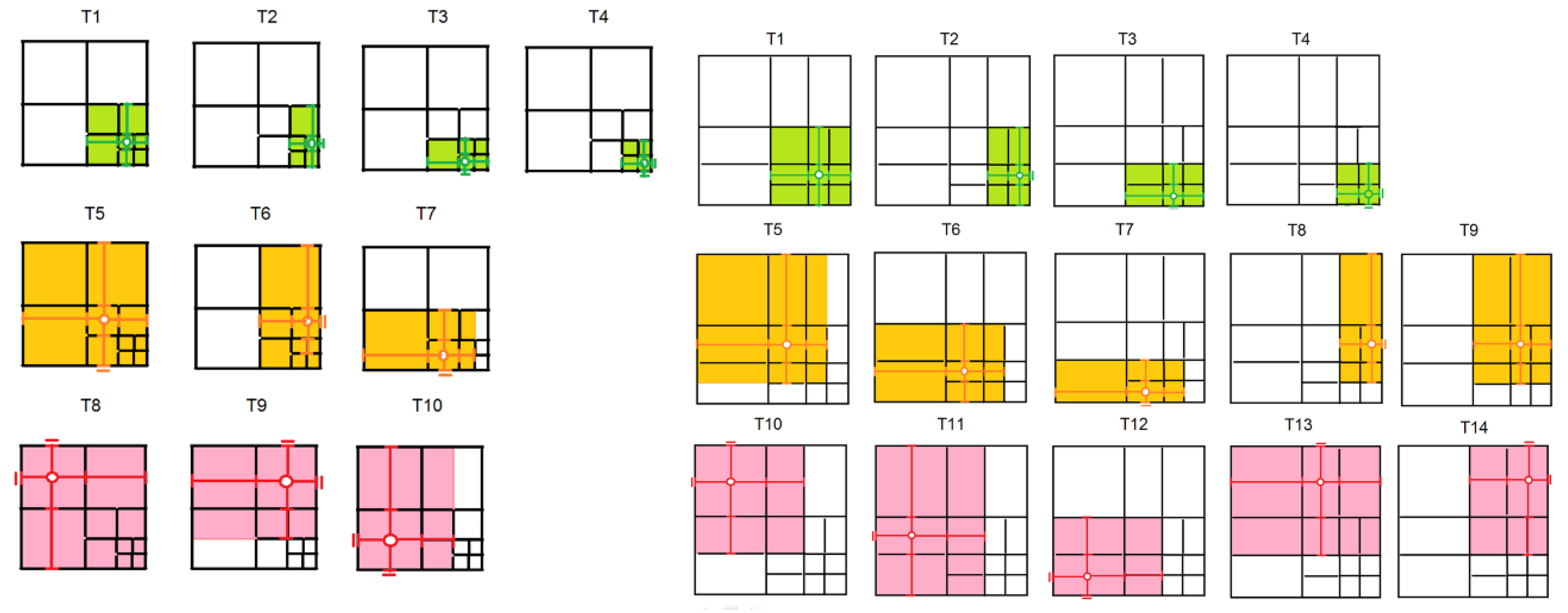
In this case, each T-spline of order p “crosses” p corresponding edges. In Figure 11, we select one T-spline related to one finite element, for the case of p = 2. We color this element in blue. We also color in green all the elements with T-splines that overlap (have non-zero support intersections) with the T-spline corresponding to the blue element. The number of green elements represents the size of the frontal matrix. To eliminate the blue element (the row related to the T-spline over the blue element), we need to subtract this row from all the rows representing the T-splines denoted by green color. In Figure 12, we plot the analogous situation, this time for p = 4. Due to the fact that the support of elements now spans into four elements in both direction, we have to denote all the elements by green color.

The elimination algorithm is the following. In the first step (i = 0), the algorithm will eliminate the small corner element. In the second step (I = 1), the algorithm will eliminate 3 elements which are neighboring the corner element. In the third step (i = 2), the algorithm will eliminate 3 elements neighboring the 3 elements eliminated in the second step. The algorithm will follow the presented scheme step by step, eliminating, in each step, 3 elements neighboring the three elements eliminated in the previous step. So, for p = 2, in each step i = 0, 1, …, we will eliminate a rows from the matrix bxb, where a = 1 for i = 0 and a = 3 for i ≥ 1. The value of b is equal to 6 + (r − i), where r denotes the number of refinement levels (for the mesh from Figure 12, r equals 4). To sum up, for i ≥ 1, we have a = 3 and b = 6 + (r − i), so the cost of elimination of 3 elements in step i is ab² = 3(6 + r − i)². We have r layers. The number of all elements in the mesh N is equal to 3*r + 1. The computational cost of elimination of elements of i-th layer is 3 (6 + r − i)². The computational cost of the whole elimination process is:

3 + Σ_i = _1,…,r−1 3(6 + r − i)² = O(r³) = O(N³)

(5)

because N = 3r + 1. For one element, for a given p ≥ 4, we obtain a dense matrix of size bxb, where b is equal to N and can eliminate 1 row. So the computational cost of elimination of one T-spline for p ≥ 4 is O(N²). Summing up, the computational cost of elimination of N elements for p ≥ 4 is

O(NN²) = O(N³)

(6)

4.2. Mesh with Edge Singularity

Now, we focus on meshes refined towards the edge. This kind of mesh is common in simulations involving, e.g., boundary layers with strong local gradients in one direction. Figure 13 presents an exemplary two-dimensional mesh with edge singularity. For this kind of mesh, each T-spline of order p “crosses” p/2 + 1 corresponding edges. Figure 13 presents the supports of corner T-splines for the cases of p = 2 and p = 4.

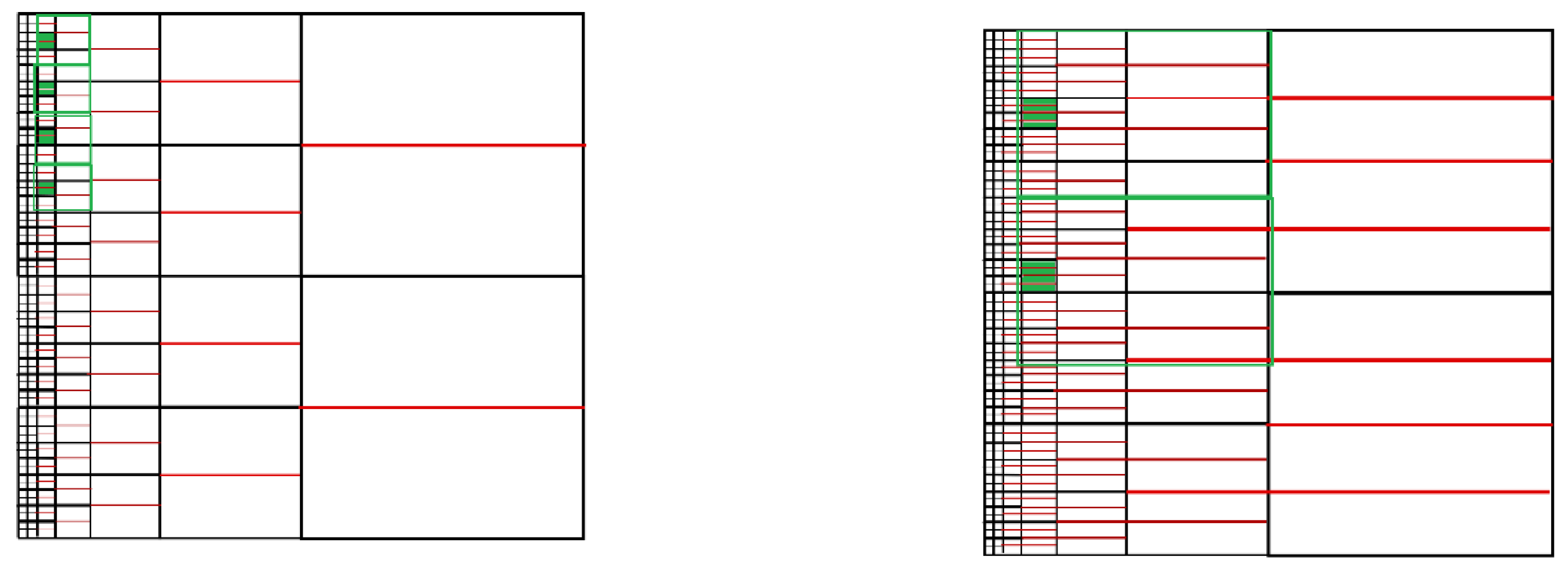
In order to eliminate one element, we have to consider p − 1 neighboring elements in each “direction”. We introduce the refinement layers as presented in the picture. Notice that the first two layers have elements of identical sizes. For simplicity, we will omit the first layer in our consideration. Each T-spline of the even order can be associated with a single element, where it has its maximum value. When we build the linear equations system resulting from finite element method discretization, in the rows and columns, we have particular T-splines span over the mesh. The entries in the matrix correspond to integrals with multiplications of the T-spline pairs (and their derivatives, depending on the problem we solve). One from a row and one from a column. Thus, non-zero entries denote overlapping supports of pairs of T-splines. In the following figures, for each T-spline whose element is denoted by blue color, we color in green all the T-spline elements whose supports overlap with the blue T-spline (see Figure 14, central and right panel and Figure 15). In this way, we denote the sparsity pattern of the matrix’s rows associated with the blue T-splines.

We have r + 1 layers (see Figure 14, where layers are denoted by different colors). The layer number 0 consists of 2^r elements. The i-th layer (i ≥ 1) consists of 2^r−i+1 elements. The number of all elements in the mesh N (equal to the number of T-splines) is equal to:

2^r + 2^r + 2^r−1 + 2^r−2 + 2^r−3 + … + 2¹ = 2^r + 2(2^r − 1) = O(2^r)

(7)

In the first step (i = 1), the algorithm will consider the number of blocks depending on the number of refinement levels in the mesh, denoted by r, and the order of approximation, denoted by p. The size of each block depends only on the order of approximation p. Then, there are the following steps for constructing blocks and eliminating selected T-splines from the blocks. We follow the layers of the mesh. For simplicity, the layer called i = 0 will be omitted. In the first step, we construct blocks related to the first layer of elements, where we group elements in the following way. We take p elements from the first layer and we denote them by blue color. Later, we search for the largest elements whose T-spline overlaps with the blue elements from the first layer. We construct a rectangular block spanning up to the largest blocks overlapping with our blue elements. In this way, we have all the “columns” of T-splines related to the non-zero entries in the rows on the blue elements in the block. For p = 2 and for i = 1, we will construct a block consisting of six elements from the first layer and three elements from the second layer. For p = 4 and for i = 1, we will construct a block consisting of 20 elements from the first layer, ten elements from the second layer, and five elements from the third layer. We noticed that the supports of the p central T-splines from two adjacent blocks do not overlap. In the next step, we construct a new, bigger rectangular block consisting of two adjacent blocks from the previous step and the next layer’s corresponding elements. For p = 2 and for i = 2, we will construct a block consisting of 12 elements from the first layer, six elements from the second layer, and three elements from the third layer. For p = 4 and for i = 2, we will construct a block consisting of 40 elements from the first layer, 20 elements from the second layer, ten elements from the third layer, and five elements from the fourth layer (see Figure 16). The size of the block in the i-th step (the number of elements in the block from the first layer of elements) is equal to n1 = (p + 1) 2^(p/2)2⁽ⁱ⁻¹⁾ = (p + 1)2^(p/2+i−1) (where (p + 1) denotes the number of elements on the largest layer in the block, (p + 1)2^(p/2) is the number of elements in the first layer in the block from the first iteration i = 1, and (p + 1)2^(p/2) 2⁽ⁱ⁻¹⁾ is the number of elements in the first layer in the block from iteration i).

The number of elements in the first layer (i = 1) is equal to 2^r. The number of blocks constructed in the i-th step is equal to:

2^r/n1 = 2^r/((p + 1)(2^(p/2)2ⁱ2⁽⁻¹⁾)) = O(2^{(r−i−p/2)}/(p))

(8)

The computational cost of elimination of T-splines from one block in the i-th step is equal to ab², where a and b are defined as:

a = 2^(p/2) + 2^(p/2)p(i-1) = O(2^(p/2)p i)

(9)

(this is because in one considered layer, we have 2^(p/2) elements to eliminate, and in the other layers, we have a total of (2^(p/2)p(i-1)) elements to eliminate)

b = (p + 1)(1 + 2 + … + p/2) + 2^(p/2) + 2^(p/2)2p(i-1) = O(2^(p/2)p i)

(10)

(since we have p + 1 elements in one layer, and two times more in the previous layers, so the total number is (p + 1)(1 + 2 + 2² + … + 2^p/2)). Thus, we have:

ab² = O((2^(p/2)p i)³)

(11)

The computational cost of the whole elimination process is:

Σ_i=1,…,r [(2^{(r−i−p/2)}/p) (2^(p/2)p i)³] = 2^r2^pp²Σ_i=1,…,r 2⁻ⁱ i³ = O(2^r2^pp²) = O(N2^pp²)

(12)

since the term Σ_i=1,…,r 2⁻ⁱ i³ converges to the constant.

5. Refined Meshes with Analysis Suitable T-Splines

This section presents the estimations of the computational costs of adaptive grids with analysis-suitable T-spline basis functions. The grids considered here have analysis-suitable T-junction extensions.

5.1. Mesh with Point Singularity

Figure 17 presents an exemplary 2D mesh with T-junctions with a point singularity for p = 2 and p = 4. In Figure 18, Figure 19, Figure 20 and Figure 21, we select one T-spline related to one finite element, for the case of p = 2. We color this element in blue. We also color in green all the elements with T-splines that overlap (have non-zero support intersections) with the T-spline corresponding to the blue element. The number of green elements represents the size of the frontal matrix. In Figure 22, Figure 23, Figure 24 and Figure 25, we plot the analogous situation, this time for p = 4. Let us start with the mesh from Figure 17 and p = 2. In the first step (i = 0), the algorithm will eliminate the corner element. In the second step (i = 1), the algorithm will eliminate three elements which are neighboring the corner element. In the third step (i = 2), the algorithm will eliminate five elements neighboring the three elements eliminated in the second step. In the fourth step (i = 3), the algorithm will eliminate five elements neighboring the five elements eliminated in the third step.

The algorithm will follow the presented scheme step by step, eliminating, in each step, five elements neighboring the five elements eliminated in the previous step. In a similar way, for p = 4, the algorithm will eliminate one element for step i = 0, three elements for step i = 1, five elements for step i = 2, and seven elements in each step i ≥ 3.

To sum up, we will eliminate T-splines, layer by layer, starting from the corner element (left top). The cost of elimination of each element can be estimated by checking the number of “layers” of other elements which have assigned T-splines who overlap elements from the current layer, by determining the support of eliminated elements (p/2) and the number of elements in such a “layer” (p + 3). So, for one layer, we have:

a = p + 3, b< = p/2(p + 3) = O(p²/2)

(13)

The computational cost of elimination of T-splines for one layer is:

ab² = O(p⁵)

(14)

We have r layers (the refinement level is r). The number of all elements in the mesh N is equal to:

1 + 3 + (3 + 2) + (3 + 2 + 2) + … + [3 + 2p/2](r − p/2) = O(rp)

(15)

The computational cost of elimination of elements of one layer is O(p⁵). The computational cost of the whole elimination process is:

Number of levels ⋅ p⁵ = rp⁵ = O(Np⁴)

(16)

5.2. Mesh with Edge Singularity

Figure 26 presents an exemplary 2D mesh with T-junctions with an edge singularity for p = 2 and p = 4. There are the following steps for constructing blocks and eliminating selected T-splines from the blocks. For simplicity, the first p/2 + 1 layers will be omitted. In the first step, we construct blocks related to the first layer of elements, where we group elements in the following way.

We take p elements from the first layer and we denote them by green color. Later, we search for the largest T-spline element overlaps with the green elements from the first layer. We construct a rectangular block spanning up to the largest blocks overlapping with our green elements. In this way, we have all the “columns” of T-splines related to the non-zero entries in the rows of the blue elements in the block. For p = 2 and for i = 1, we will construct a block consisting of six elements from the first layer and three elements from the second layer. For p = 4 and for i = 1, we will construct a block consisting of 20 elements from the first layer, ten elements from the second layer, and five elements from the third layer (see the right panel in Figure 26).

We noticed that the supports of the p central T-splines from two adjacent blocks do not overlap. In the next step, we construct a new, bigger rectangular block consisting of two adjacent blocks from the previous step and the next layer’s corresponding elements. For p = 2 and for i = 2, we will construct a block composed of 12 elements from the first layer, six elements from the second layer, and three elements from the third layer. For p = 4 and for i = 2, we will construct a block consisting of 40 elements from the first layer, 20 elements from the second layer, ten elements from the third layer, and five elements from the fourth layer (see the right panel in Figure 27). The size of the block in the i-th step (the number of elements in the first column of elements in the block) is equal to (p + 1):

2^(p/2)2⁽ⁱ⁻¹⁾ = (p + 1)2 2^(p/2+i−1)

(17)

The number of all elements in the first layer (i = 1) is equal to 2^r. As such, the number of blocks constructed in the i-th step is equal to:

2^r/((p + 1)(2^(p/2)+i−1)) = O(2^r−i−p/2/(p + 1)

(18)

The number of all elements in one layer (i-th layer) is equal to 2^r−i. Thus, the number of all elements in the considered layers is equal to:

N = Σ_{i=1,…,r−p/2+1}(2^r−i) = O(2 ^r)

(19)

The computational cost of elimination of T-splines from one block in the i-th step is equal to ab², where a and b are defined as:

a = 2^p/2 + 2^(p/2)p(i-1) = O(2^p/2pi)

(20)

(this is because in the actual layer, we have 2 ^(p/2) elements, and in the other layers, we have 2^(p/2)p(i-1) elements)

b = (p + 1)(1 + 2 + … + p/2) + 2^p/2 + 2^(p/2)2p(i-1) = O(2^(p/2)pi)

(21)

(since we have p + 1 elements in one layer, and this number multiplies by 2 in each following layer, we have (p + 1)(1 + 2 + 2²…2^p/2)). Thus.

ab² = O((2^p/2pi)³)

(22)

The number of blocks considered in the i-th iteration is equal to:

2^r/((p + 1)(2^(p/2)2ⁱ 2⁽⁻¹⁾)) = O(2^{(r−i−p/2)}/(p))

(23)

Thus, the computational cost of the whole elimination process is equal to the sum over layers from the number of blocks in the layer, times the cost for the layer:

Σ_{i=1,…,r−p/2+1} [((2^{(r−p/2−i)}/p ((2^(p/2) p i)³)] = 2^r 2^p p² = O(2^r 2^p p²) = O(N 2^p p²)

(24)

6. Numerical Results

In this section we present the numerical results, obtained in Octave, confirming the estimated computational costs for T-splines and analysis-suitable T-splines with our ordering algorithms. They are summarized in Figure 27, Figure 28, Figure 29, Figure 30, Figure 31 and Figure 32. For T-splines, the matrices are dense and cost of factorization is O(N³). For analysis-suitable T-splines, for grids refined towards a point or an edge, our ordering delivers linear computational cost of factorization. For analysis-suitable T-splines, for grids refined towards an edge, our recursive ordering algorithm delivers a linear computational cost, which is up to 50-times faster than alternative Octave orderings.

7. Conclusions

In this paper, we estimated, for the first time, the computational costs of the multi-frontal solver when using T-spline and analysis-suitable T-splines on uniform and adaptive grids. We have shown that analysis-suitable T-splines have a linear computational cost on adaptive grids. We also proposed an ordering algorithm permuting the rows and columns of the resulting sparse matrix such that the computational cost of factorization is linear for grids refined towards point and edge singularities when using analysis-suitable T-splines. Our ordering algorithm constructs a binary tree, with nodes assigned to elements on levels of the refinement. The root is the largest element, and the leaves are the smallest elements. It orders the elements and T-splines assigned to them by post-order traversal of the tree.

In this paper, we compared computational costs of isogeometric analysis with T-splines and analysis-suitable T-splines. We focused on model two-dimensional symmetry-preserving grids, including a uniform grid, a grid refined to a point, and a grid refined to an edge. They are building blocks for adaptive two-dimensional grids. We conclude that the cost for a uniform grid is O(N^1.5p³) for both T-splines and analysis-suitable T-splines, as well as for B-splines (since supports of T-splines are equivalent to the supports of B-splines on uniform grids). The number of unknowns on the uniform grid is defined as N = O(2^2sp²), where 2^2s is the number of elements and p denotes the T-splines (or B-splines) order. The cost for grids refined towards a point is O(N³) for T-splines and O(Np⁴) for analysis-suitable T-splines. For T-splines, the number of unknowns is N = 3r + 1 = O(r), where r is the number of layers in the mesh. For analysis-suitable T-splines, the number of unknowns is N = O(rp). Finally, the costs for grids refined towards an edge is O(N2^pp²) for both T-splines and analysis-suitable T-splines. The number of unknowns for T-splines and analysis-suitable T-splines is O(2^r), where r is the number of refinement levels. However, the constant in front of the order is larger for analysis-suitable T-splines.

In conclusion, we advocate the use of analysis-suitable T-splines. It is a well-known fact that the numerical accuracy of the finite element method simulations on analysis-suitable grids is higher than on grids without the T-junctions extensions. Besides other advantages from the approximability theory, they also result in a lower computational cost of multi-frontal direct solvers. Future work may involve developing estimates for three-dimensional grids and other kinds of basis functions utilized in isogeometric analysis computations.

References

1. Cottrell, A.; Hughes, T.J.R.; Bazilevs, Y. Isogeometric Analysis: Toward Unification of CAD and FEA; John Wiley and Sons: Hoboken, NJ, USA, 2009. [Google Scholar]
2. Bazilevs, Y.; Calo, V.M.; Cottrell, J.A.; Evans, J.A.; Lipton, S.; Scott, M.A.; Sederberg, T.W. Isogeometric analysis using T-splines. Comput. Methods Appl. Mech. Eng. 2010, 199, 229–263. [Google Scholar] [CrossRef] [Green Version]
3. Bornemann, P.B.; Cirak, F. A subdivision-based implementation of the hierarchical B-spline finite element method. Comput. Methods Appl. Mech. Eng. 2013, 253, 584–598. [Google Scholar] [CrossRef]
4. Giannelli, C.; Juttler, B.; Speleers, H. THB-splines: The truncated basis for hierarchical splines. Comput. Aided Geom. Des. 2012, 29, 485–498. [Google Scholar] [CrossRef] [Green Version]
5. Dokken, T.; Lyche, T.; Pettersen, K. Polynomial splines over locally refined box-partitions. Comput. Aided Geom. Des. 2013, 30, 331–356. [Google Scholar] [CrossRef]
6. Johannessen, K.; Kvamsdal, T.; Dokken, T. Isogeometric analysis using LR B-splines. Comput. Methods Appl. Mech. Eng. 2014, 269, 471–514. [Google Scholar] [CrossRef] [Green Version]
7. Burkhart, D.; Hamann, B.; Umlauf, G. Iso-geometric Finite Element Analysis Based on Catmull-Clark: Subdivision Solids. Comput. Graph. Forum 2010, 29, 1575–1584. [Google Scholar] [CrossRef]
8. Wei, X.; Zhang, Y.; Hughes, T.J.R.; Scott, M. Truncated hierarchical Catmull-Clark subdivision with local refinement. Comput. Methods Appl. Mech. Eng. 2015, 291, 1–20. [Google Scholar] [CrossRef]
9. Wei, X.; Zhang, Y.; Hughes, T.J.R.; Scott, M. Extended Truncated hierarchical Catmull-Clark subdivision with local refinement. Comput. Methods Appl. Mech. Eng. 2016, 299, 316–336. [Google Scholar] [CrossRef] [Green Version]
10. Li, X.; Wei, X.; Zhang, Z. Hybrid non-uniform recursive subdivision with improved convergence rates. Comput. Methods Appl. Mech. Eng. 2019, 352, 606–624. [Google Scholar] [CrossRef]
11. Amestoy, P.R.; Duff, I.S. Multifrontal parallel distributed symmetric and unsymmetric solvers. Comput. Methods Appl. Mech. Eng. 2000, 184, 501–520. [Google Scholar] [CrossRef] [Green Version]
12. Amestoy, P.R.; Duff, I.S.; Koster, J.; L’Excellent, J.-L. A fully asynchronous multifrontal solver using distributed dynamic scheduling. SIAM J. Matrix Anal. Appl. 2001, 1, 15–41. [Google Scholar] [CrossRef] [Green Version]
13. Amestoy, P.R.; Guermouche, A.; L’Excellent, J.-Y.; Pralet, S. Hybrid scheduling for the parallel solution of linear systems. Comput. Methods Appl. Mech. Eng. 2001, 2, 136–156. [Google Scholar] [CrossRef] [Green Version]
14. Collier, N.; Pardo, D.; Dalcin, L.; Paszyński, M.; Calo, V.M. The cost of continuity: A study on performance of isogeometric finite elements using direct solvers. Comput. Methods Appl. Mech. Eng. 2012, 213–216, 353–361. [Google Scholar] [CrossRef]
15. Paszyński, M.; Pardo, D.; Calo, V.M. Direct solvers performance on h-adapted grids. Comput. Math. Appl. 2015, 70, 282–295. [Google Scholar] [CrossRef] [Green Version]
16. Garcia, D.; Pardo, D.; Dalcin, L.; Paszyński, M.; Collier, N.; Calo, V.M. The value of continuity: Refined isogeometric analysis and fast direct solvers. Comput. Methods Appl. Mech. Eng. 2017, 316, 586–605. [Google Scholar] [CrossRef] [Green Version]
17. Heggernes, P.; Eisenstat, S.C.; Kumfert, G.; Pothen, A. The Computational Complexity of the Minimum Degree Algorithm; ICASE Report No. 2001–42; Institute for Computer Applications in Science and Engineering: Hampton, VA, USA, 2001. [Google Scholar]
18. Schulze, J. Toward a tighter coupling of bottom-up and top-down sparse matrix ordering methods. BIT 2001, 41, 800. [Google Scholar] [CrossRef]
19. Karypis, G.; Kumar, V. A fast and high quality multilevel scheme for partitioning irregular graphs. SIAM J. Sci. Comput. 1998, 20, 359–392. [Google Scholar] [CrossRef]
20. Liu, J.W.H. The multifrontal method for sparse matrix solution: Theory and practice. SIAM Rev. 1992, 34, 82–109. [Google Scholar] [CrossRef]
21. Paszyńska, A.; Paszyński, M.; Jopek, K.; Woźniak, M.; Goik, D.; Gurgul, P.; AbouEisha, H.; Moshkov, M.; Calo, V.M.; Lenharth, A.; et al. Quasi-optimal elimination trees for 2D grids with singularities. Sci. Program. 2015, 2015, 303024. [Google Scholar] [CrossRef]
22. Paszyńska, A. Volume and neighbors algorithm for finding elimination trees for three dimensional h-adaptive grds. Comput. Math. Appl. 2014, 68, 1467–1478. [Google Scholar] [CrossRef]
23. AbouEisha, H.; Moshkov, M.; Calo, V.; Paszynski, M.; Goik, D.; Jopek, K. Dynamic programming algorithm for generation of optimal elimination trees for multi-frontal direct solver over h-refined grids. Procedia Comput. Sci. 2014, 29, 947–959. [Google Scholar] [CrossRef] [Green Version]
24. AbouEisha, H.; Calo, V.M.; Jopek, K.; Moshkov, M.; Paszyńska, A.; Skotniczny, M. Element partition trees for h-refined meshes to optimize direct solver performance. Part 1, Dynamic programming. Int. J. Appl. Math. Comput. Sci. 2017, 27, 351–365. [Google Scholar] [CrossRef] [Green Version]
25. Balay, S.; Abhyankar, S.; Adams, M.F.; Brown, J.; Brune, P.; Buschelman, K.; Eijkhout, V.; Gropp, W.D.; Kaushik, D.; Knepley, M.G.; et al. PETSc Web Page. 2014. Available online: http://www.mcs.anl.gov/petsc (accessed on 12 October 2020).
26. Blackford, L.S.; Choi, J.; Cleary, A.; D’Azevedo, E.; Demmel, J.; Dhillon, I.; Dongarra, J.; Hammarling, S.; Henry, S.; Petitet, A.; et al. ScaLAPACK Users’ Guide; Society for Industrial and Applied Mathematics: Philadelphia, PA, USA, 1999. [Google Scholar]
27. Hnon, P.; Ramet, P.; Roman, J. PaStiX: A High-Performance Parallel Direct Solver for Sparse Symmetric Definite Systems. Parallel Comput. 2002, 28, 301–321. [Google Scholar] [CrossRef]
28. Li Xiaoye, S. An Overview of SuperLU: Algorithms, Implementation, and User Interface. Trans. Math. Softw. 2005, 31, 302–325. [Google Scholar]
29. Gurgul, P. A Linear Complexity Direct Solver for H-adaptive Grids with Point Singularities. Procedia Comput. Sci. 2014, 29, 1090–1099. [Google Scholar] [CrossRef] [Green Version]
30. Da Veiga, L.B.; Buffa, A.; Sangalli, G.; Vazquez, R. Analysis-suitable T-splines of arbitrary degree: Definition and properties. Math. Models Methods Appl. Sci. 2013, 23, 1979–2003. [Google Scholar] [CrossRef]
31. Calo, V.M.; Collier, N.; Pardo, D.; Paszyński, M. Computational complexity and memory usage for multi-frontal direct solvers used in p finite element analysis. Procedia Comput. Sci. 2011, 4, 1854–1861. [Google Scholar] [CrossRef] [Green Version]
32. Skotniczny, M. Computational Complexity of Hierarchically Adapted Meshes. In Computational Science—ICCS 2020, Proceedings of the 20th International Conference, Amsterdam, The Netherlands, 3–5 June 2020; Lecture Notes in Computer Science; Springer: Cham, Switzerland, 2020; Volume 12139, pp. 226–239. [Google Scholar]
33. Gomez, H.; Calo, V.M.; Bazilevs, Y.; Hughes, T.J.R. Isogeometric analysis of the Cahn-Hilliard phase-field model. Comput. Methods Appl. Mech. Eng. 2008, 197, 4333–4352. [Google Scholar] [CrossRef]
34. Gomez, H.; Hughes, T.J.R.; Nogueira, X.; Calo, V.M. Isogeometric analysis of the isothermal Navier-Stokes-Korteweg equations. Comput. Methods Appl. Mech. Eng. 2010, 199, 1828–1840. [Google Scholar] [CrossRef]
35. Hsu, M.-C.; Akkerman, I.; Bazilevs, Y. High-performance computing of wind turbine aerodynamics using isogeometric analysis. Comput. Fluids 2011, 49, 93–100. [Google Scholar] [CrossRef]
36. Duddu, R.; Lavier, L.; Hughes, T.J.R.; Calo, V.M. A finite strain Eulerian formulation for compressible and nearly incompressible hyper-elasticity using high-order NURBS elements. Int. J. Numer. Methods Eng. 2012, 89, 762–785. [Google Scholar] [CrossRef]
37. Calo, V.M.; Brasher, N.; Bazilevs, Y.; Hughes, T.J.R. Multiphysics Model for Blood Flow and Drug Transport with Application to Patient-Specific Coronary Artery Flow. Comput. Mech. 2008, 43, 161–177. [Google Scholar] [CrossRef]
Figure 1. C0 B-spline basis functions defined by tensor product of knot vectors [0 0 0 1 2 2 2] × [0 0 0 1 2 2 2].
Symmetry 12 02070 g001
Figure 2. (Left panel): The sparse matrix resulting from finite element method discretizations with C0 B-spline basis functions defined by tensor product of knot vectors [0 0 0 1 2 2 2] × [0 0 0 1 2 2 2]. (Right panel): The elimination graph of the matrix.
Symmetry 12 02070 g002
Figure 3. (Left panel): The separators found by the nested dissections algorithm, using the peripheral node 23 as the starting node. (Right panel): The elimination tree.
Symmetry 12 02070 g003
Figure 4. (Left panel) T-splines defined over a grid refined towards a point. (Right panel) Analysis-suitable T-splines defined over a grid refined towards a point.
Symmetry 12 02070 g004
Figure 5. Ordering of elements = T-splines = rows of matrices for grids refined towards a point and an edge.
Symmetry 12 02070 g005
Figure 6. (Left panel): The exemplary mesh consisting of 26⋅32 elements (s = 3, p = 2). (Right panel): The exemplary mesh consisting of 24⋅52 elements (s = 2, p = 4).
Symmetry 12 02070 g006
Figure 7. (Left panel): Iteration step i = 0, p = 2, and s = 3. The elements for which the T-splines can be eliminated are denoted by green color. (Right panel): Iteration step i = 1, p = 2, and s = 3. The elements for which the T-splines can be eliminated are denoted by light green color, elements for which the T-splines were eliminated in previous steps are denoted by white color, and the rest of elements are denoted by blue color.
Symmetry 12 02070 g007
Figure 8. Iteration step i = 2, p = 2, and s = 3. The elements for which the T-splines can be eliminated are denoted by dark green color, elements for which the T-splines were eliminated in the previous steps are denoted by white color, and the rest of elements are denoted by blue color.
Symmetry 12 02070 g008
Figure 9. Iteration step i = 0 and I = 1, p = 4. The elements for which the T-splines can be eliminated are denoted by green color, elements for which the T-splines were eliminated in previous steps are denoted by white color, and the rest of elements are denoted by blue color.
Symmetry 12 02070 g009
Figure 10. Iteration step i = 2 and I = 3, p = 4. The elements for which the T-splines can be eliminated are denoted by green color, elements for which the T-splines were eliminated in previous steps are denoted by white color, and the rest of elements are denoted by blue color.
Symmetry 12 02070 g010
Figure 11. We select a single element and its T-spline and we denote it by blue color. Next, we browse all equal-size and larger elements, and we mark in green these elements whose T-splines have non-zero intersections with the T-spline span over the blue element. We consider quadratic T-splines here.
Symmetry 12 02070 g011
Figure 12. The elements with T-splines having non-zero intersection with the T-spline corresponding to the element, denoted by blue color, are denoted by green color, for p = 4.
Symmetry 12 02070 g012
Figure 13. Two-dimensional mesh with edge singularity. Supports of T-splines of order p = 2 (left panel) and p = 4 (right panel) on meshes with edge singularity.
Symmetry 12 02070 g013
Figure 14. (Left panel): Layers of mesh refined toward the edge. Central panel and (right panel): The sparsity pattern of the rows of the matrix associated with the blue T-splines from the first and the second considered column, for p = 2.
Symmetry 12 02070 g014
Figure 15. The support of the T-spline related with an element from the first (left panel), second (central panel), or third layer (right panel), denoted by blue color, overlapping with supports of other T-splines, denoted by green color, for p = 2, 4, and 6, respectively.
Symmetry 12 02070 g015
Figure 16. Eliminated blocks for p = 2 and 4 for the first, second, and third iteration steps.
Symmetry 12 02070 g016aSymmetry 12 02070 g016b
Figure 17. The exemplary 2D meshes with a point singularity and T-junction extensions for p = 2 and p = 4 (left and right, respectively).
Symmetry 12 02070 g017
Figure 18. Layer i = 0 for p = 2.
Symmetry 12 02070 g018
Figure 19. Layer i = 1 for p = 2.
Symmetry 12 02070 g019
Figure 20. Layer i = 2 for p = 2.
Symmetry 12 02070 g020
Figure 21. Layer i = 3 for p = 2.
Symmetry 12 02070 g021
Figure 22. Layer i = 0 for p = 4.
Symmetry 12 02070 g022
Figure 23. Layer i = 1 for p = 4.
Symmetry 12 02070 g023
Figure 24. Layer i = 2 for p = 4.
Symmetry 12 02070 g024
Figure 25. Layer i = 4 for p = 4.
Symmetry 12 02070 g025aSymmetry 12 02070 g025b
Figure 26. Exemplary 2D mesh with edge singularity and T-junction extensions.Left panel denotes p = 2, right panel denotes p = 4.
Symmetry 12 02070 g026
Figure 27. Exemplary blocks for p = 2 and p = 4 for the first iteration step (upper panel). Exemplary blocks for p = 2 and the first, second, and third iteration steps (bottom panel).
Symmetry 12 02070 g027aSymmetry 12 02070 g027b
Figure 28. Execution times and sparsity of a matrix for a mesh with T-splines, p = 2, refined towards a point.
Symmetry 12 02070 g028
Figure 29. Execution times and sparsity of a matrix for a mesh with T-splines, p = 4, refined towards a point.
Symmetry 12 02070 g029
Figure 30. Execution times and sparsity of a matrix for a mesh with analysis-suitable T-splines, p = 2, refined towards a point, permuted with our ordering.
Symmetry 12 02070 g030
Figure 31. Execution times and sparsity of a matrix for a mesh with analysis-suitable T-splines, p = 4, refined towards a point, permuted with our ordering.
Symmetry 12 02070 g031
Figure 32. Comparison of Approximate Minimum Degree (AMD) and Cuthill–McKee orderings, available in Octave, and our ordering for a matrix for a mesh with analysis-suitable T-splines refined towards an edge, p = 2, permuted with our ordering.
Symmetry 12 02070 g032
Publisher’s Note: MDPI stays neutral with regard to jurisdictional claims in published maps and institutional affiliations.