Article

A Multivariate Long Short-Term Memory Neural Network for Coalbed Methane Production Forecasting

1
College of Resources and Environment, University of Chinese Academy of Sciences, Beijing 100049, China
2
School of Earth Sciences and Engineering, Hohai University, Nanjing 211000, China
3
Key Laboratory of Computational Geodynamics, College of Earth and Planetary Sciences, University of Chinese Academy of Sciences, Beijing 100049, China
*
Authors to whom correspondence should be addressed.
Symmetry 2020, 12(12), 2045; https://doi.org/10.3390/sym12122045
Submission received: 17 November 2020 / Revised: 3 December 2020 / Accepted: 6 December 2020 / Published: 10 December 2020

Abstract

:
Owing to the importance of coalbed methane (CBM) as a source of energy, it is necessary to predict its future production. However, the production process of CBM is the result of the interaction of many factors, making it difficult to perform accurate simulations through mathematical models. We must therefore rely on the historical data of CBM production to understand its inherent features and predict its future performance. The objective of this paper is to establish a deep learning prediction method for coalbed methane production without considering complex geological factors. In this paper, we propose a multivariate long short-term memory neural network (M-LSTM NN) model to predict CBM production. We tested the performance of this model using the production data of CBM wells in the Panhe Demonstration Area in the Qinshui Basin of China. The production of different CBM wells has similar characteristics in time. We can use the symmetric similarity of the data to transfer the model to the production forecasting of different CBM wells. Our results demonstrate that the M-LSTM NN model, utilizing the historical yield data of CBM as well as other auxiliary information such as casing pressures, water production levels, and bottom hole temperatures (including the highest and lowest temperatures), can predict CBM production successfully while obtaining a mean absolute percentage error (MAPE) of 0.91%. This is an improvement when compared with the traditional LSTM NN model, which has an MAPE of 1.14%. In addition to this, we conducted multi-step predictions at a daily and monthly scale and obtained similar results. It should be noted that with an increase in time lag, the prediction performance became less accurate. At the daily level, the MAPE value increased from 0.24% to 2.09% over 10 successive days. The predictions on the monthly scale also saw an increase in the MAPE value from 2.68% to 5.95% over three months. This tendency suggests that long-term forecasts are more difficult than short-term ones, and more historical data are required to produce more accurate results.

1. Introduction

Coalbed methane (CBM) is an important unconventional clean energy source that has the potential to eventually replace natural gas. As such, it is attracting increasing attention from around the world. Accurate prediction of CBM production can not only forecast the economic benefits of CBM, but also provide advice for the establishment of mining plans, which play an important role in the production process of CBM. However, CBM is subject to a range of complex interactions relevant to the many factors involved in its creation [1]. These unique features have led to its classification as an unconventional gas resource [2]. Therefore, accurate production forecasts for CBM present certain challenges. At present, the prediction methods for CBM production mainly include the type curve and decline curve methods [3], numerical simulation methods [4], material balance methods [5], and machine learning methods, including neural networks [6] and support vector machines (SVMs) [7] among others.
The type curve and decline curve methods have been widely used for production analysis, achieving important results. Fetkovich [8] proposed the first-generation production type curve, which subsequent type curves have improved upon. Aminian et al. [2] proposed a series of curves that could predict CBM and water production, studying the effects of different parameters on these curves and discussing their applications and limitations, the most notable of which being the difficulty in representing a uniform model at the production cycle’s different stages. Jang et al. [9] used the method of decline curve analysis and combined material balance and fluid state analysis to predict the production dynamics of CBM, subsequently establishing a comprehensive production data model. Decline curve analysis is currently the most commonly used and effective yield forecasting method, but it also has its limitations [10].
The numerical simulation method uses a complicated mathematical model. When using this method, it is necessary to obtain enough production data and measure geological parameters as accurately as possible [6]. These factors will have a very large impact on the production simulation. Therefore, if these influencing factors cannot be accurately obtained, the numerical simulation method will not be used. A detailed description of numerical simulation techniques can be found in [11]. Numerical simulation technology is increasingly used in unconventional gas reservoirs, and more and more geological factors are taken into consideration. Li et al. [12] used geological survey and experimental data to study the formation history of coalbed methane reservoirs and analyzed the role of various stages in the process of coalbed methane production. Zhou et al. [13] used numerical simulation technology to predict production and believed that the skin factor and coal shrinkage rate have important impacts on CBM production. Thararoop et al. [14] proposed a numerical simulation model that took into account the water in the coal matrix and the swelling and shrinkage of coal. In addition, numerical simulation software for coalbed methane reservoirs, whose development was based on the C++ programming language, was proposed in [15]. Numerical simulation technology requires sufficient geological data to provide support, but it is difficult to obtain these factors in actual production. Complex mathematical models also limit the application of this method.
Material balance is also an important method for estimating the reserves of coalbed methane, since this method can comprehensively consider the influence of many factors. In [5], two material balance methods were proposed, which were used to predict unconventional gas reservoirs and estimate the original gas, respectively. The difference between this method and the traditional material balance method is that the influence of adsorbed gas is taken into account. Shi et al. [16] established a material balance equation to estimate coalbed methane reserves, taking into account factors such as dissolved gas and free gas. Sun et al. [17] used a flow material balance equation, combined with the relationship between pressure and saturation, to analyze the production of low-permeability CBM wells and achieved good results. More and more material balance models that consider multiple factors have been developed. However, the actual production of coalbed methane is a dynamic process. The influencing factors are complex and diverse, and it is impossible to take all of them into consideration. Additionally, similar to the numerical simulation method, it is very difficult to obtain many factors, so the material balance equation is also restricted in the prediction of coalbed methane reserves.
The development of machine learning provides a new method for forecasting the production of CBM. Compared with the previous method, the advantage of machine learning is that it does not need to obtain the geological conditions of the coalbed methane reservoir and can make predictions only from the production data. For example, the back propagation (BP) neural network method can efficiently predict production without having to understand the conditions of coalbed methane reservoirs or deal with insufficient production data [6]. Xia et al. [18] achieved favorable results through their proposal of a hybrid method to forecast CBM production capacity. This method takes both the rough set (RS) and least-square support vector machine models into consideration. Huang and Wang [7] optimized their own SVM using a genetic algorithm (GA), and their results showed that their GA-SVM model could also achieve high accuracy in CBM production capacity predictions. The machine learning method has the characteristics of being simple and convenient to implement, and it does not need to consider the complex factors in the actual process, so it is widely used in production forecasting. However, traditional machine learning methods, such as SVM, the Bayes method [19], multiple regression analysis [20,21], and neural networks do not consider time dependence when processing time series data. Therefore, the use of such methods to predict CBM production also has limitations.
The actual production process of CBM is very complicated, involving the interaction of geological factors and human factors. However, the production data of CBM has certain rules, which reflects the production process of CBM to a certain extent. As such, it is possible to predict future production by focusing on inherent laws and tendencies based on the available historical data rather than complex process research. This can be accomplished through long short-term memory neural networks (LSTM NNs). LSTM NNs are deep learning recurrent neural network structures with the ability to process long-term sequence data [22]. These networks can learn the inherent laws present in historical data through a time series without having to consider complex coal seam environments. LSTMs can also be applied to other fields such as environmental science, in which some scholars have applied LSTM models to predict PM2.5 concentrations in air pollution, achieving valuable results [22,23,24,25]. In terms of public transportation, Chen et al., Tian et al., and Li and Cao [26,27,28] used the LSTM model to study traffic flow. In [29], LSTMs were used to forecast traffic speed in the Beijing area. Petersen et al. [30] used CNNs (Convolutional Neural Networks) and LSTMs to predict bus travel time. In the financial sector, Fischer and Krauss [31] and Kim and Won [32] applied the LSTM model to market forecasts and achieved superior results to those of random forests methods and deep neural networks (DNNs). Vochozka et al. [33] used the LSTM model to establish a method for predicting company bankruptcy, which provided a reference for the company’s future development. In the industrial and energy sectors, Wu et al. [34] used the LSTM network to estimate the remaining service life of an engineering system, while Peng et al. [35] used LSTMs and differential evolution to predict the price of electricity, and the prediction accuracy was superior to current models. Sagheer and Kotb [36] proposed a genetic algorithm-optimized deep LSTM method to predict oil production, which has proven to be more accurate than statistical and software calculation methods. Although the LSTM model has been widely used in research related to production and price prediction, it is rarely applied in the research of unconventional gas reservoirs. Xu et al. [37] used LSTM networks to predict the production of coalbed methane and achieved good results. However, this study did not consider the influence of multiple factors and only used coalbed methane production data.
In view of the complexity and limitations of the current methods, the objective of this article is to propose an artificial intelligence-based method for CBM production forecasting. This paper proposes the use of multivariate LSTM NNs as a prediction method for CBM production. Auxiliary data such as casing pressure, water production, and bottom hole temperatures are also inputted into the LSTM NN to improve prediction performance. This combined model was validated using production data from a CBM well; its results were compared with those obtained using a traditional LSTM NN model. The results demonstrated that auxiliary data can improve the prediction outcome. In addition, this paper proposes a multi-step prediction method more in line with the time process of CBM production, as forecasting performances will deteriorate as time lag increases.

2. Data and Methods

2.1. Data Description

The data used in the experiment were coalbed methane production data in the Panhe Demonstration Area in the Qinshui Basin of China, totaling 1945 days of recorded data. The Qinshui Basin was the first CBM development base of high rank coal reservoirs in China. The daily log included the current CBM production, casing pressure, water production, and bottom hole temperature (including both highest and lowest temperatures). The data did not take into account geological factors such as rock formations, coal seam thickness, and burial depth, because these may not have been data that changed over time. The time series of these five variables is shown in Figure 1, where the abscissa represents the time and the ordinate represents the value recorded on that day. It can be easily noted that there exists a periodic correlation between the five aforementioned variables. As can be seen from the figure, the CBM production data of this well can be roughly divided into three phases: the drainage phase, the high yield phase, and the steady phase. The drainage phase was from 0 to 600 days, during which the CBM production was extremely unstable or very low. The high yield phase was from 600 to 1000 days, during which the continuous high yield of CBM was achieved, and the water yield was almost zero. After 1000 days was basically the steady phase of this well. The CBM production was basically stable and the CBM well almost no longer produced water. There are more complex divisions of the CBM production phases. Here, we simply divided the process into three phases for the purpose of subsequent prediction process analysis and cross-validation. In fact, in the early stage (0–600 days) of CBM production, due to the instability of the casing pressure and water production, the production of CBM was very unstable and difficult to predict. In addition, the actual production should also take into account the influence of human factors in the early stage, so we did not consider the early production stage forecast because it was very difficult. When the water production dropped to very little and remained stable, the production of CBM rose rapidly at this time and maintained a relatively stable state, showing a certain regularity.
Before a prediction could be made, the input data needed to be preprocessed. It was necessary that the input data be normalized, as the range of values for each variable was quite different. In this case, we utilized the min-max normalization method, as seen in Formula (1), to make all input variables take values between 0 and 1. It is important to note that the time series data were recorded daily with no missing values, thus making any data interpolation unnecessary. We could then convert the normalized time series data into a supervised learning problem. Because of the phases of CBM production, it was necessary to have sufficient training data and cover each phase of the production process. To evaluate the accuracy of the model while also ensuring adequate orientation for the model, the first 1600 days of data were used as a training set, while the remaining 345 days were used as a test set:
y n o r m =   y i   m i n y i m a x y i   m i n y i
where ynorm is the normalized value, min(yi) is the smallest value of the dataset, and max(yi) is the maximum value of the dataset.

2.2. M-LSTM NN Model

In this study, the traditional LSTM NN was improved using multivariate inputs. The overall framework of the multivariate LSTM NN (i.e., multivariate long short-term memory (M-LSTM)) model is shown in Figure 2. LSTM NN is a kind of recurrent neural network (RNN), but it can solve the problem of gradient explosion well when traditional RNNs analyze long time sequences [38]. Details on RNNs and LSTM NNs are given in Appendix A and Appendix B.
In our prediction model, the input variables were divided into two parts (shown in the blue solid box in Figure 2): the first was CBM production data, and the second was auxiliary production record data (casing pressure, water production, and the bottom hole temperatures). Suppose we were to predict the CBM production at time t. The input data would be the historical data at time t-1. Again, note that the input data had been normalized and transformed into a supervised learning problem. Two or more hidden stacked LSTM layers are included in a green dashed box in Figure 2. The LSTM network structure was used to determine the inherent features from the historical input data to predict CBM production at time t. Both the number of LSTM layers and nodes in each layer were optimized through experimentation. We then used a fully connected dense layer to obtain the forecast result of the daily production of coalbed methane. After inputting the long-term series of production data into the LSTM layer, it took multiple iterations to obtain the corresponding features.

2.3. Evaluation Index

In order to optimize the model parameters and evaluate the model’s accuracy, three indicators were used in this paper: root mean square error (RMSE), mean absolute error (MAE), and mean absolute percentage error (MAPE). The calculation formula of the three indexes is as follows:
MAE =   1 n i = 1 n P i A i
MAPE =   1 n i = 1 n P i A i A i
RMSE =   1 n i = 1 n P i A i 2
where Pi represents the model predicted value, Ai represents the true value, and n is the number of days of testing.

2.4. Network Architecture

In order to achieve the predicted structure of CBM production shown in Figure 2, it was necessary to establish some initial parameters for the network, such as the number of LSTM layers, the number of nodes in each of these, the number of dense layers, the number of nodes in each of these, the learning rate, the batch size, and the gradient descent function among others. We explored the influence of each parameter on network performance under the condition that other parameters were fixed during this process. The optimum values were selected by the most favorable RMSE, MAE, and MAPE values. The initial parameters of the model were 2 LSTM hidden layers, 1 dense layer, and a batch size of 72. The computer specifications for the experiment were as follows. The CPU was an Intel(R) Core(TM) i7-7700; the RAM was 32.00 GB; and the GPU was an NVIDIA GeForce GTX 1060 3 GB.
In the process of model parameter selection and model accuracy validation, cross-validation was needed. However, when it came to the time series data, traditional methods, such as the leave-one-out method and K-fold cross-validation, were not applicable because of time dependence. For the time series, nested cross-validation was a very good choice. Therefore, rolling origin recalibration evaluation was adopted in this paper [39]. It is a method of nested cross-validation of a time series. The process of nested cross-validation of the time series is shown in Figure 3. In the figure, the blue boxes represent training data, the red boxes represent validation data, the yellow boxes represent test data, and the white boxes represent unused data. We split the data into 7 processes and averaged the results of the 7 processes to calculate the final error of the model. We used 100 days of data each time as the validation data and moved it to the training data of the next process in chronological order.
We then examined the influence of the number of nodes in each hidden layer of the LSTM model. For simplification purposes, we selected the number of hidden layer nodes from an alternative set of {32, 64, 128, 256, 512}, which was determined from previous experience. The prediction performance (shown in Table 1) indicated that our M-LSTM model achieved optimal performance with 128 nodes. Increasing the number of nodes to 256 did not improve the prediction performance but did increase the training time of the network. Finally, when the number of nodes was increased to 512, the accuracy of the model decreased rapidly, as indicated by the MAE, MAPE, and RMSE.
Having fixed the number of hidden layer nodes to 128, we next investigated the effects of different learning rates. The learning rate was also selected from an alternative set of {0.005, 0.001, 0.0005, 0.0001, 0.00005}. The results (shown in Table 2) demonstrated that the training results of the larger learning rate were poor, which was because the larger learning rate caused the model to miss the optimal parameters. As the learning rate gradually decreased, the accuracy of the model was significantly improved. When the learning rate continued to decrease from 0.0001, the accuracy was not significantly improved. Therefore, considering efficiency and accuracy, the learning rate was set to 0.0001. This was due to the value of the learning rate being crucial to the training of the model; in other words; having too large a learning rate led to shock in the training process, and having too small a learning rate made it difficult for the model to reach convergence.

3. Results and Discussion

3.1. Prediction Performance

Once the initial network parameters were fixed, the M-LSTM NN model was instructed with the aforementioned training set until convergence was reached. The accuracy of the network was then evaluated using the test set, and the resulting predicted and actual CBM production values are shown in Figure 4. It is shown that the predicted production values were generally consistent with the actual values, as most of the points were near the y = x line. Obtaining an R2 value between the predicted and actual CBM production indicated that 94.4% of the variance was successfully described by the M-LSTM NN model.

3.2. Comparison with Traditional LSTM NN Model (without Multivariate Inputs)

To verify the importance of the auxiliary data (casing pressure, water production, and bottom hole temperatures) for CBM production prediction, we established an LSTM NN model without these inputs and compared its accuracy with that of the M-LSTM model. At the same time, and in order to avoid accidental errors in the experiment, after the optimal network structure was trained, 30 experiments were conducted on the LSTM NN and M-LSTM NN models, respectively, and the error distribution of both models was statistically analyzed. Thirty independent repeated experiments were sufficient to obtain a good error distribution. The boxplot distribution of the RMSE, MAE, and MAPE values is shown in Figure 5. The results demonstrate that the test errors obtained by the M-LSTM NN model were significantly smaller than those of the traditional LSTM NN model. Table 3 shows the average error over 30 experiments. Compared with the predicted results of the LSTM NN model (MAPE = 1.14%), the predicted results of the M-LSTM NN model (MAPE = 0.91%) were closer to the actual value. Thus, it can be inferred that using additional production data (casing pressure, water production, and bottom hole temperatures) as auxiliary inputs can significantly improve the prediction accuracy of CBM production.
We further explored the influence of each variable on the prediction results. Only one auxiliary variable was input into the M-LSTM network at a time to predict the production of coalbed methane. The results obtained are shown in Table 4. It can be found that casing pressure and water production as auxiliary variables could improve prediction accuracy, of which water production improved it the most (MAPE = 1.01%). However, the input of temperature variables had almost no effect on the prediction results.

3.3. Multi-Step Predictions

Following the development of our M-LSTM model to predict daily CBM production, we continued our study through a multi-step forecast model. In the multi-step models, each time step prediction was compared with the actual production data for the next day. This actual data, taken from the test set, was then made available to the model for the next time step prediction. As an example, Figure 6 shows how a two-step model predicted the production over three days. In Step 1 (that is, from time t), we must forecast the time t + 1, t + 2, and t + 3. In Step 2, from time t + 1, we must forecast the time t + 2, t + 3, and t + 4, and so on. This type of model mimics real-world CBM production scenarios, as new CBM production data is obtained each day and used to predict future production.
In our model, the daily production of CBM was predicted in five time steps, spanning a time period of ten days for each step. The network structure in our experiment included two LSTM layers and a fully connected dense layer. As shown in Table 5, the accuracy of the five initial time steps was noted for each of the next ten days. These results demonstrated that with an increase in each predicted time interval, the performance of the model grew worse, with the MAPE value increasing from 0.24% to 2.09% from the first to the tenth day. It can be inferred from these results that long-term predictions are more difficult than short-term predictions, requiring more historical data to establish sufficient training for the model.
In the actual production process of CBM, it is often more common to focus on the monthly production of CBM rather than production on any given day. With this in mind, we scaled the CBM production data and converted daily production into monthly production. After this scaling, we were able to obtain 65 months of production data. We made five time step forecasts for the previous eight months, with predictions for the next three months in each step. The multi-step predictions’ results of monthly coalbed methane production are shown in Table 6, where we can see that comparatively similar results were obtained from the multi-step prediction of daily output. The MAPE values for this iteration of the model increased from 2.68% to 5.95%. As the time interval increased again, the predicted production values began to deviate further from the actual values. Although the performance of the model worsened with an increase in each time interval, the error (MAPE = 5.95%) still fell into an acceptable range.

4. Conclusions

A multivariate long short-term memory neural network (M-LSTM NN) model for coalbed methane production forecasting was proposed in this paper. Due to the optimization of the parameters presented in the model (including the number of LSTM NN hidden layer nodes, learning rate, and others), as well as the subsequent results, we were able to reach the following conclusions from our study:
(1) The M-LSTM NN model we developed was able to achieve favorable results in predicting CBM production. The results show that the use of deep neural networks to predict CBM production can achieve good results without considering complex geological factors and by only using historical production data. The M-LSTM network provides a fast artificial intelligence prediction method for CBM production.
(2) Thirty independent and repeated experiments were conducted, comparing the results of LSTM NN models without additional auxiliary inputs and our own M-LSTM NN model, with MAE, MAPE, and RMSE values indicating that the M-LSTM NN model achieved better results than LSTM NN model. In addition, we analyzed the impact of each variable on the results and found that water production and casing pressure can improve the accuracy of the prediction, while inputting the temperature into the M-LSTM network did not improve the results. This shows that the bottom hole temperature has almost no effect on the production of CBM in the actual production process of CBM, and inputting it into the M-LSTM network cannot improve prediction accuracy. Since we have only obtained very little auxiliary production information, we cannot analyze the factors that have the highest impact on CBM production forecasts. Therefore, in future research, it is necessary to select those variables that are highly correlated with CBM production.
(3) A multi-step predictions model was also developed that was more consistent with the actual production processes of CBM, utilizing historical as well as current data to predict future CBM production. During our experimenting process, it was found that prediction accuracy was inversely related to the increase in time lag, regardless of whether the CBM production in question was at daily or monthly intervals. This finding suggests that to successfully predict term CBM production, more historical data may be needed to calibrate and train future models.

Author Contributions

X.X. established the prediction model, reached the conclusion, and wrote the main part of the paper. X.R. proposed a research framework for the study. Y.F. and T.Y. modified the introduction and checked the grammar of the article. Finally, Y.J. provided data processing methods and provided suggestions on the structure of the article. All authors have read and agreed to the published version of the manuscript.

Funding

This research was funded by the National Key Research and Development Program of China (Grant No. 2019YFC1804304), the National Science and Technology Major Project of China (Grant No. 2017ZX05064005; 2016ZX05066006), the Fundamental Research Funds for the Central Universities (Grant No. 2019B02514), the Strategic Priority Research Program of the Chinese Academy of Sciences (Grant No. XDA05030100), and the National Natural Science Foundation of China (Grant No. 41771478).

Conflicts of Interest
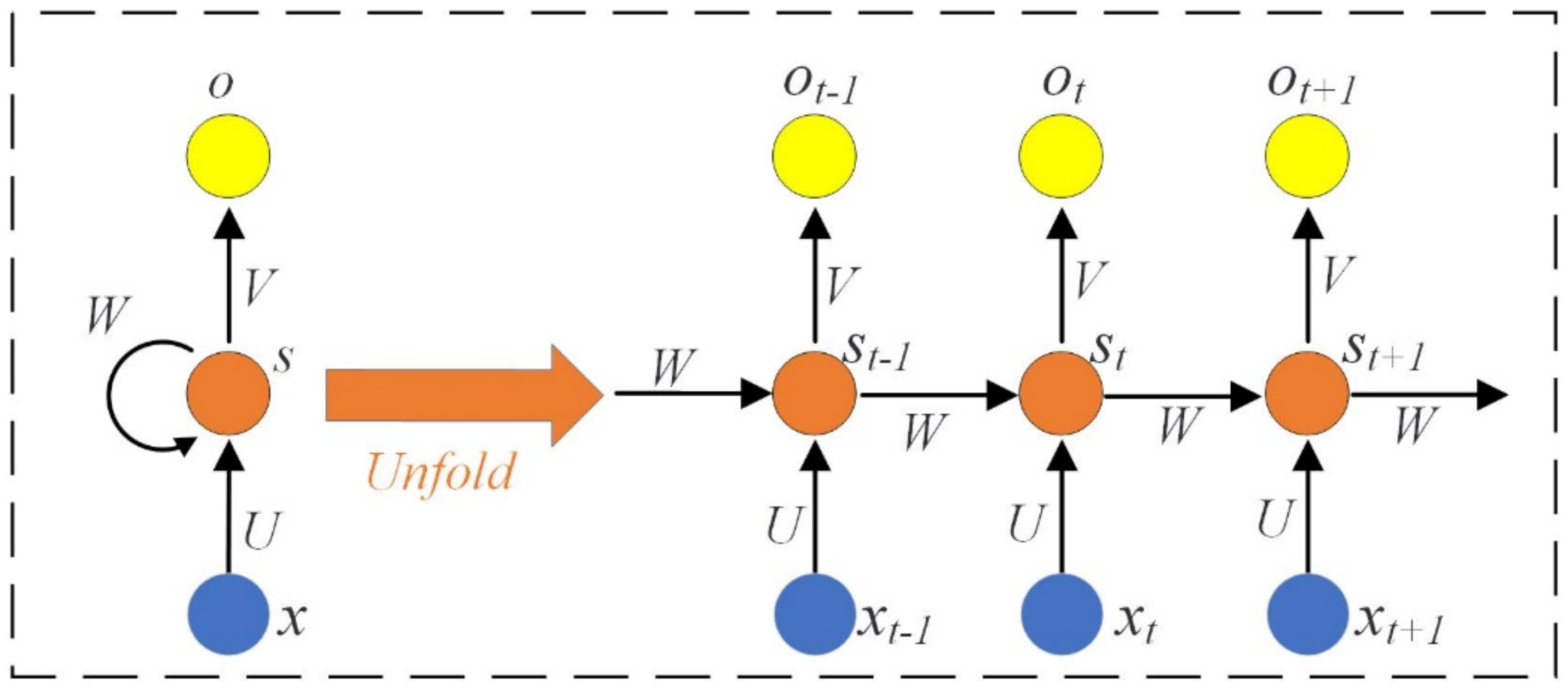
The authors declare no conflict of interest.

Appendix A. RNN

RNNs are commonly used neural networks for dealing with time series problems. Different from general neural networks, RNNs have memory units so they can capture time series information. Figure A1 shows the network structure of RNNs. xt, Ot, and St represent the input, memory, and output, respectively, at time t. W, U, and V represent the weights between the input layer, hidden layer, and output layer, respectively. Because the weights between different layers of RNNs are shared, the network parameters can be greatly reduced. RNNs may cause gradient disappearance or gradient explosion when calculating connections between nodes with a long time interval [35]. Therefore, RNNs can only deal with short-term problems and cannot solve long-term dependence problems. CBM production is related over a long period of time, so RNNs cannot be used directly to predict it.
Figure A1. A typical recurrent neural network (RNN) network structure.
Symmetry 12 02045 g0a1

Appendix B. LSTM NN

LSTM NNs can overcome the problem of gradient disappearance in RNNs in the back propagation process [38]. Based on RNNs, the LSTM method improves the memory unit of the hidden layer. The memory unit of an LSTM NN is shown in Figure A2.
LSTM NNs use three gates to solve the problem that RNNs cannot handle long-term sequences: input gates, forget gates, and output gates. The input, output and memory state of an LSTM NN at time t are xt, ht, and Ct respectively. The memory state Ct is defined as follows:
c t = f t C t 1 + i t t a n   h W x c x t + W h c h t 1 + b c
where ft is the forget gate, it is the input gate, and W and b are the corresponding weights and offsets.
The function of the input gate is to control the input of data. The calculation formula for the input gate is as follows:
i t = σ W x i x t + W h i h t 1 + W c i C t 1 + b i
where σ is the sigmoid function.
The function of the forget gate is to decide which information to keep and discard the unnecessary information. The formula for the forget gate is as follows:
f t = σ W x f x t + W h f h t 1 + W c f C t 1 + b f
The function of the output gate is to control the output information. It can be calculated by the following formula:
o t = σ W x o x t + W h o h t 1 + W c o C t + b o
The definition of ht is as follows:
h t = o t t a n   h c t
where tan h is the hyperbolic tangent.
Figure A2. An LSTM network hidden layer cell structure.
Symmetry 12 02045 g0a2

References

  1. Stopa, J.; Mikolajczak, E. Empirical modeling of two-phase CBM production using analogy to nature. J. Pet. Sci. Eng. 2018, 171, 1487–1495. [Google Scholar] [CrossRef]
  2. Aminian, K.; Ameri, S. Predicting production performance of CBM reservoirs. J. Nat. Gas Sci. Eng. 2019, 1, 25–30. [Google Scholar] [CrossRef]
  3. Clarkson, C.R. Production data analysis of unconventional gas wells: Review of theory and best practices. Int. J. Coal Geol. 2013, 109, 101–146. [Google Scholar] [CrossRef]
  4. Clarkson, C.R. Production data analysis of unconventional gas wells: Workflow. Int. J. Coal Geol. 2013, 109–110, 147–157. [Google Scholar] [CrossRef]
  5. King, G.R. Material-balance techniques for coal-seam and devonian shale gas-reservoirs with limited water influx. SPE Reserv. Eng. 1993, 8, 67–72. [Google Scholar] [CrossRef]
  6. Lue, Y.; Tang, D.; Xu, H.; Tao, S. Productivity matching and quantitative prediction of coalbed methane wells based on BP neural network. Sci. China Technol. Sci. 2011, 54, 1281–1286. [Google Scholar] [CrossRef]
  7. Huang, X.D.; Wang, S.Q. Prediction of Bottom-Hole Flow Pressure in Coalbed Gas Wells Based on GA Optimization SVM; IEEE: New York, NY, USA, 2018. [Google Scholar]
  8. Fetkovich, M.J. Decline curve analysis using type curves. J. Pet. Technol. 1980, 32, 1065–1077. [Google Scholar] [CrossRef]
  9. Jang, H.; Kim, Y.; Park, J.; Lee, J. Prediction of production performance by comprehensive methodology for hydraulically fractured well in coalbed methane reservoirs. Int. J. Oil Gas Coal Technol. 2019, 20, 143–168. [Google Scholar] [CrossRef]
  10. Li, P.; Hao, M.; Hu, J.; Ru, Z.; Li, Z. A new production decline model for horizontal wells in low-permeability reservoirs. J. Pet. Sci. Eng. 2018, 171, 340–352. [Google Scholar] [CrossRef]
  11. Cipolla, C.L.; Lolon, E.P.; Erdle, J.C.; Rubin, B. Reservoir Modeling in Shale-Gas Reservoirs. SPE Reserv. Eval. Eng. 2010, 13, 638–653. [Google Scholar] [CrossRef]
  12. Li, L.C.; Wei, C.T.; Qi, Y.; Cao, J.; Wang, K.Y.; Bao, Y. Coalbed methane reservoir formation history and its geological control at the Shuigonghe Syncline. Arab. J. Geosci. 2015, 8, 619–630. [Google Scholar] [CrossRef]
  13. Zhou, F.D. History matching and production prediction of a horizontal coalbed methane well. J. Pet. Sci. Eng. 2012, 96–97, 22–36. [Google Scholar] [CrossRef]
  14. Thararoop, P.; Karpyn, Z.T.; Ertekin, T. Development of a multi-mechanistic, dual-porosity, dual-permeability, numerical flow model for coalbed methane reservoirs. J. Nat. Gas Sci. Eng. 2012, 8, 121–131. [Google Scholar] [CrossRef]
  15. Yun, M.G.; Rim, M.W.; Han, C.N. A model for pseudo-steady and non-equilibrium sorption in coalbed methane reservoir simulation and its application. J. Nat. Gas Sci. Eng. 2018, 54, 342–348. [Google Scholar] [CrossRef]
  16. Shi, J.T.; Chang, Y.C.; Wu, S.G.; Xiong, X.Y.; Liu, C.; Feng, K. Development of material balance equations for coalbed methane reservoirs considering dewatering process, gas solubility, pore compressibility and matrix shrinkage. Int. J. Coal Geol. 2018, 195, 200–216. [Google Scholar] [CrossRef]
  17. Sun, Z.; Shi, J.; Zhang, T.; Wu, K.; Miao, Y.; Feng, D.; Li, X. The modified gas-water two phase version flowing material balance equation for low permeability CBM reservoirs. J. Pet. Sci. Eng. 2018, 165, 726–735. [Google Scholar] [CrossRef]
  18. Xia, H.M.; Qin, Y.C.; Zhang, L.J.; Cao, Y.P.; Xu, J.X. Forecasting of Coalbed Methane (CBM) Productivity Based on Rough Set and Least Squares Support Vector Machine. In Proceedings of the 2017 25th International Conference on Geoinformatics, Buffalo, NY, USA, 2–4 August 2017. [Google Scholar]
  19. Zhao, C.; Li, J. Equilibrium Selection under the Bayes-Based Strategy Updating Rules. Symmetry 2020, 12, 739. [Google Scholar] [CrossRef]
  20. Zhang, B.; Xu, D.; Liu, Y.; Li, F.; Cai, J.; Du, L. Multi-scale evapotranspiration of summer maize and the controlling meteorological factors in north China. Agric. For. Meteorol. 2016, 216, 1–12. [Google Scholar] [CrossRef]
  21. Zhang, Y.; Huang, P. Influence of mine shallow roadway on airflow temperature. Arab. J. Geosci. 2020, 13, 12. [Google Scholar] [CrossRef]
  22. Bai, Y.; Zeng, B.; Li, C.; Zhang, J. An ensemble long short-term memory neural network for hourly PM2.5 concentration forecasting. Chemosphere 2019, 222, 286–294. [Google Scholar] [CrossRef]
  23. Li, X.; Peng, L.; Yao, X.; Cui, S.; Hu, Y.; You, C.; Chi, T. Long short-term memory neural network for air pollutant concentration predictions: Method development and evaluation. Environ. Pollut. 2017, 231, 997–1004. [Google Scholar] [CrossRef] [PubMed]
  24. Wen, C.; Liu, S.; Yao, X.; Peng, L.; Li, X.; Hu, Y.; Chi, T. A novel spatiotemporal convolutional long short-term neural network for air pollution prediction. Sci. Total Environ. 2019, 654, 1091–1099. [Google Scholar] [CrossRef] [PubMed]
  25. Zhao, J.; Deng, F.; Cai, Y.; Chen, J. Long short-term memory—Fully connected (LSTM-FC) neural network for PM2.5 concentration prediction. Chemosphere 2019, 220, 486–492. [Google Scholar] [CrossRef] [PubMed]
  26. Chen, W.; Zheng, Z.; Liu, J.; Chen, P.; Wu, X. LSTM network: A deep learning approach for short-term traffic forecast. IET Intell. Transp. Syst. 2017, 11, 68–75. [Google Scholar]
  27. Tian, Y.; Zhang, K.; Li, J.; Lin, X.; Yang, B. LSTM-based traffic flow prediction with missing data. Neurocomputing 2018, 318, 297–305. [Google Scholar] [CrossRef]
  28. Li, Y.; Cao, H. Prediction for Tourism Flow based on LSTM Neural Network. In 2017 International Conference on Identification, Information and Knowledge in the Internet of Things, Qufu, China, 19–21 October 2017; Qufu Normal University, School of Information Science and Engineering: Shandong, China, 2018; Volume 129, pp. 277–283. [Google Scholar]
  29. Ma, X.; Tao, Z.; Wang, Y.; Yu, H.; Wang, Y. Long short-term memory neural network for traffic speed prediction using remote microwave sensor data. Transp. Res. Part C Emerg. Technol. 2015, 54, 187–197. [Google Scholar] [CrossRef]
  30. Petersen, N.C.; Rodrigues, F.; Pereira, F.C. Multi-output bus travel time prediction with convolutional LSTM neural network. Expert Syst. Appl. 2019, 120, 426–435. [Google Scholar] [CrossRef] [Green Version]
  31. Fischer, T.; Krauss, C. Deep learning with long short-term memory networks for financial market predictions. Eur. J. Oper. Res. 2018, 270, 654–669. [Google Scholar] [CrossRef] [Green Version]
  32. Kim, H.Y.; Won, C.H. Forecasting the volatility of stock price index: A hybrid model integrating LSTM with multiple GARCH-type models. Expert Syst. Appl. 2018, 103, 25–37. [Google Scholar] [CrossRef]
  33. Vochozka, M.; Vrbka, J.; Suler, P. Bankruptcy or Success? The Effective Prediction of a Company’s Financial Development Using LSTM. Sustainability 2020, 12, 7529. [Google Scholar] [CrossRef]
  34. Wu, Y.; Mei, Y.; Dong, S.; Li, L.; Liu, Y. Remaining useful life estimation of engineered systems using vanilla LSTM neural networks. Neurocomputing 2018, 167–179. [Google Scholar] [CrossRef]
  35. Peng, L.; Liu, S.; Liu, R.; Wang, L. Effective long short-term memory with differential evolution algorithm for electricity price prediction. Energy 2018, 162, 1301–1314. [Google Scholar] [CrossRef]
  36. Sagheer, A.; Kotb, M. Time series forecasting of petroleum production using deep LSTM recurrent networks. Neurocomputing 2019, 323, 203–213. [Google Scholar] [CrossRef]
  37. Xu, X.X.; Rui, X.P.; Fan, Y.L.; Yu, T.; Ju, Y.W. Forecasting of Coalbed Methane Daily Production Based on T-LSTM Neural Networks. Symmetry 2020, 12, 861. [Google Scholar] [CrossRef]
  38. Li, C.; Wang, Z.; Rao, M.; Belkin, D.; Song, W.; Jiang, H.; Xia, Q. Long short-term memory networks in memristor crossbar arrays. Nat. Mach. Intell. 2019, 1, 49–57. [Google Scholar] [CrossRef]
  39. Bergmeir, C.; Benítez, J.M. On the use of cross-validation for time series predictor evaluation. Inf. Sci. 2012, 191, 192–213. [Google Scholar] [CrossRef]
Figure 1. The production data. (a) is the coalbed methane (CBM) production, (b) is the casing pressure, (c) is the water production, (d) is the lowest bottom hole temperature, and (e) is the highest bottom hole temperature.
Symmetry 12 02045 g001
Figure 2. The framework of the multivariate long short-term memory (M-LSTM) model for CBM daily production forecasting. The input variables (CBM production, casing pressure, and the rest) are included in a blue solid box, where n indicates the time lag. The stacked LSTM layers are included in a green dashed box. A recursive arrow indicates that processing can be repeated.
Symmetry 12 02045 g002
Figure 3. The nested cross-validation process.
Symmetry 12 02045 g003
Figure 4. Predicted and actual CBM production.
Symmetry 12 02045 g004
Figure 5. Comparison of error distribution between the M-LSTM NN model and the traditional LSTM NN model. (a) RMSE, (b) MAE and (c) MAPE.
Symmetry 12 02045 g005
Figure 6. A multi-step predictions model.
Symmetry 12 02045 g006
Table 1. The effects of different numbers of nodes in each LSTM hidden layer.
NodesRMSE (m3)MAE (m3)MAPE (%)
3281.8450.111.50
6479.3046.851.41
12875.7741.411.24
25680.8150.021.53
51284.4652.621.58
Table 2. The effects of different learning rates.
Learning RateRMSE (m3)MAE (m3)MAPE (%)
0.005142.42121.873.69
0.00195.3772.602.22
0.000582.2754.081.66
0.000176.2444.681.35
0.0000576.5943.181.30
Table 3. Average error over 30 experiments.
ModelRMSE (m3)MAE (m3)MAPE (%)
LSTM NN46.4731.461.14
M-LSTM NN42.4624.980.91
Table 4. The influence of each variable on the prediction results.
VariableRMSE (m3)MAE (m3)MAPE (%)
Casing pressure44.1531.221.10
Water production42.5428.581.01
Lowest temperature46.6431.451.14
Highest temperature46.6331.081.15
No auxiliary variables46.4731.461.14
All variables42.4624.980.91
Table 5. Prediction accuracy of multi-step predictions for CBM daily production.
Time Lag (Day)RMSE (m3)MAE (m3)MAPE (%)
t + 111.556.420.24
t + 217.3912.820.48
t + 322.5019.180.71
t + 423.7720.660.77
t + 525.0022.060.82
t + 626.1623.370.87
t + 727.2824.610.92
t + 838.5035.391.31
t + 947.5746.091.71
t + 1059.5156.742.09
Table 6. Prediction accuracy of multi-step predictions for CBM monthly production.
Time Lag (Month)RMSE (m3)MAE (m3)MAPE (%)
t + 1241022302.68
t + 2338029803.65
t + 3514048305.95
Publisher’s Note: MDPI stays neutral with regard to jurisdictional claims in published maps and institutional affiliations.

