Article

Lorentz Violation at the Level of Undergraduate Classical Mechanics

by
Madeline Clyburn
1,* and
Charles D. Lane
1,2
1
Berry College, Mount Berry, GA 30149, USA
2
IU Center for Spacetime Symmetries, Indiana University, Bloomington, IN 47405, USA
*
Author to whom correspondence should be addressed.
Symmetry 2020, 12(10), 1734; https://doi.org/10.3390/sym12101734
Submission received: 8 October 2020 / Revised: 15 October 2020 / Accepted: 15 October 2020 / Published: 20 October 2020
(This article belongs to the Section Physics)

Abstract

:
In this paper, we use the classical limit of the Standard-Model Extension to explore some generic features of Lorentz violation. This classical limit is formulated at the level of undergraduate physics. We first discuss the general equations of motion and then concentrate on three specific systems. First, we consider the theoretical aspects of pendulum motion in the presence of Lorentz violation, followed by some sample experimental results. The experimental bounds we achieve, in the range of 10 3 , are not competitive with the current bounds from atomic clocks; rather, our experiment illustrates some common ideas and methods that appear in Lorentz-violation studies. We then discuss how Newton’s 2nd Law must be treated with caution in our model. Finally, we introduce a computational simulation of a binary star system that is perturbed by Lorentz-violating effects. This simulation shows some interesting behavior that could be the subject of future analytical studies.

1. Introduction

Lorentz symmetry, comprising symmetry under rotations and boosts, is a fundamental aspect of all modern theories of physics. It is obeyed exactly in the Standard Model of quantum fields and locally in General Relativity. Due to the fundamental role Lorentz symmetry plays, it is important to test its validity as strongly as possible.
Moreover, Lorentz symmetry could be the key to experimental probes of physics at the Planck scale. It has been shown that frameworks for physics beyond the Standard Model, such as string theory [1,2] and noncommutative geometry [3,4], allow Lorentz symmetry to be broken.
The Standard-Model Extension (SME) is a general framework [5,6,7] for describing all potential violations of Lorentz symmetry that respect other common aspects of modern physics. It contains tensor-valued coefficients that parameterize Lorentz-violating interactions; these coefficients may be low-energy expectation values of fields that appear in Planck-scale physics. The SME has been used to analyze the sensitivity of precise experiments to potential Lorentz violation including probes of atomic clocks [8,9,10,11] and binary stars [12,13].
In this work, we employ the classical limit of the SME [14,15] to analyze several macroscopic systems. First, we outline the general classical model. Then, we solve the equations of motion for a simple pendulum in the presence of a Lorentz violation. We compare the model to data gathered over a span of 6 months and so extract bounds of several SME coefficients. We then briefly discuss the behavior of a block on an inclined plane; this system has been previously analyzed in the context of the classical SME, so we limit our comments to a few new points. Finally, we describe a computational model of a binary star system in the presence of a Lorentz violation. This model illustrates several core properties of the SME such as energy conservation, angular-momentum non-conservation, the precession of orbits, and forbidden regions.
Notation: We use standard index notation for vector and tensor components, including the Einstein summation convention for repeated indices. All Latin indices j , k , range from 1 to 3, corresponding to axes x, y, and z. The Kronecker delta δ j k takes the value 1 when j = k and 0 otherwise.

2. General Theory

In this section, we outline the core qualitative ideas of the Lorentz-violating SME. We then discuss how comparing sidereal variation and solar variation can help search for Lorentz-violating experimental signals. We then introduce the classical Lagrangian that displays the same behavior as the quantum-field SME at low energies and large sizes. Finally, we describe a few general consequences.

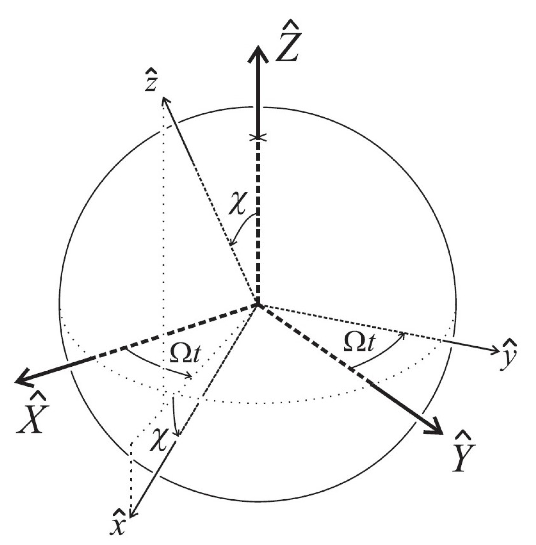
2.1. Transformations and Symmetries

Lorentz symmetry includes symmetry under boosts (changes in velocity) and under rotations (changes in orientation). Large changes in velocity (relative to the speed of light) may be difficult to achieve in undergraduate labs, but large changes in orientation are easy to design. Indeed, it is difficult to avoid large changes in orientation, as most labs are fixed on Earth’s surface as it rotates. Moreover, rotations and their physical effects are easier to visualize than boosts for many students. Therefore, this introductory paper is primarily concerned with the rotational aspect of Lorentz symmetry and its violation.
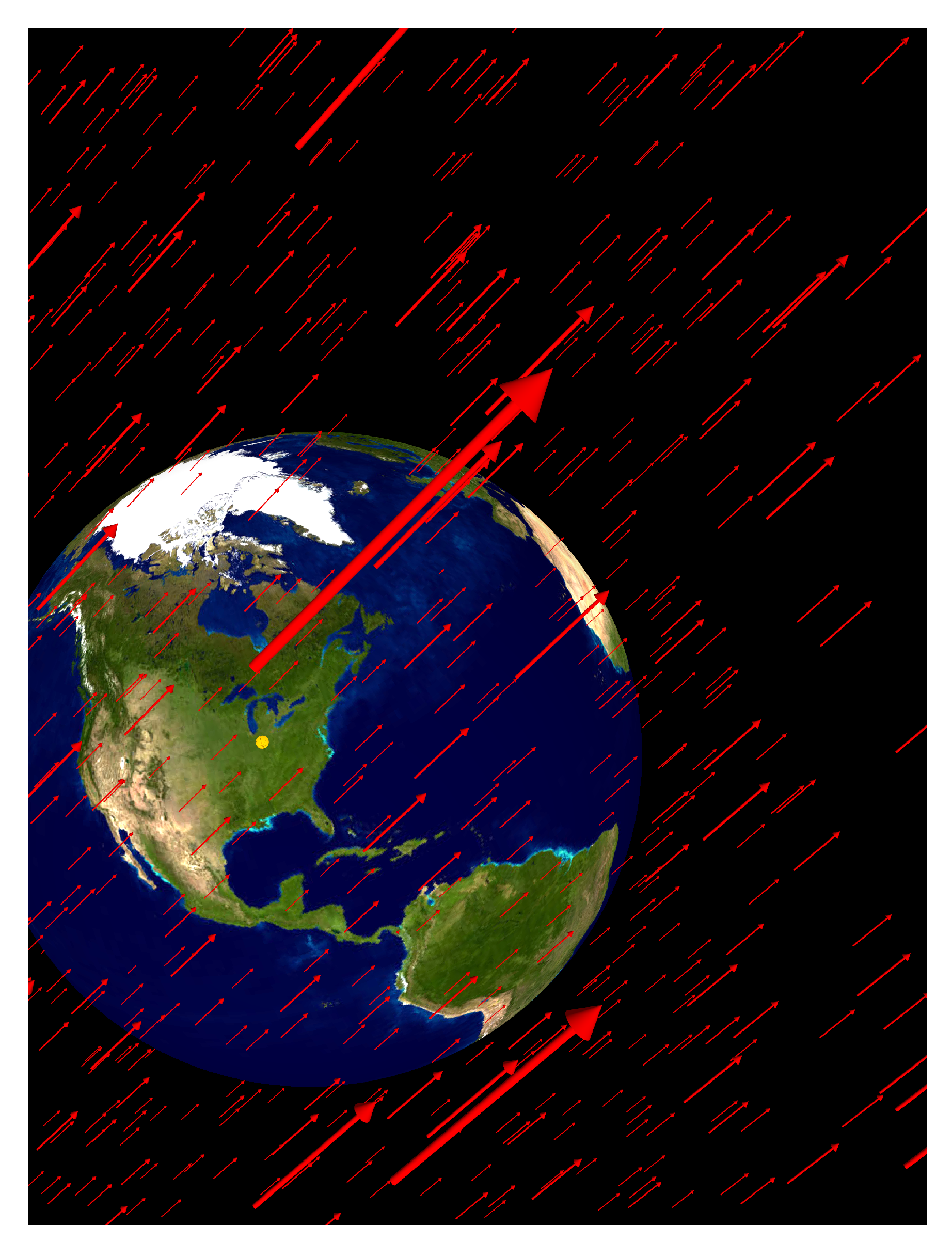
Key Idea 1: In the Standard-Model Extension, the vacuum is not symmetrical under rotations. It has a directionality to it.
One way of imagining this is to imagine that there is a very weak but omnipresent force pushing everything in the universe in some particular direction as seen in Figure 1. The direction in which things are getting pushed is different from all other directions, and so rotation symmetry is broken.
This example is correct in spirit, but cannot apply directly to the SME:
  • In the flat-spacetime limit of the SME, momentum and energy are conserved. This implies that the background vector field cannot be a force field; a background force field would generate momentum (and kinetic energy) from nothing. Instead, the background fields that appear in the SME are more abstract.
    It is reasonable to instead imagine a background torque field, i.e., a field that encourages everything in the universe to rotate around a particular axis. Such effects do occur in the SME, but they are not directly relevant to this work;
  • The background field we’ll be studying in this work is a matrix (a 2nd-rank tensor) rather than a vector. Details of its behavior appear later in this section;
  • The full SME has many fields: A torque-producing field that acts on electrons, a torque-producing field that acts on protons, and so on. The fields that act on different particles do not necessarily point in the same direction or have the same magnitude.
    Moreover, there are other effects that cannot be cleanly represented as torques: a vector field that behaves in many ways, like the electromagnetic vector potential, a matrix field that causes a particle’s kinetic energy to depend on the direction of its velocity, and so on. The fundamental goal of the SME is to include all effects that violate Lorentz symmetry while respecting most other important aspects of the Standard Model; this leads to a broad smorgasbord of effects.
Lorentz violation may be detected by searching for systems whose properties depend on their orientation with respect to background vacuum fields. For example, a pendulum that oscillates parallel to a background vector field might have a longer period than a pendulum that oscillates perpendicular to that field. An atomic clock with the atoms aligned with the background field might tick at a faster rate than a clock with the atoms aligned perpendicular to that field. The space of possible orbits in a binary star system may take different forms for systems with differently oriented initial conditions.
Key Idea 2: An important technique for searching for Lorentz violation is to create a system, such as an atomic clock, that should keep ticking at a constant rate according to conventional physics. We then watch it very carefully as it rotates with Earth through the background field.
If it speeds up and slows down in correlation with its orientation, then it has provided evidence of Lorentz violation. In Section 3.1, the “clocks” we study are pendulums that swing east and west. As Earth rotates, the east–west axis rotates through the background vacuum. Certain effects in the SME predict that the period of the pendulum will increase and decrease in correlation with Earth’s rotation.
This technique depends on the system’s orientation with respect to the rest of the universe. One way to gauge this orientation is to monitor time. For example, a system’s orientation at 6:00 p.m. is about 90 away from its orientation at noon. There is an important subtlety with this, though, that lies in the word “about” and is concerned with the difference between solar days and sidereal days. Solar days are defined by Earth’s rotation with respect to our Sun and are the basis for conventional time-keeping. Sidereal days are defined by Earth’s rotation with respect to the rest of the universe, the “background stars”. Since Earth moves around the Sun as it rotates, solar and sidereal days do not have the same length. More precisely: to complete a solar-day, Earth must rotate an additional 1/365.24 of a full rotation, which takes approximately 4 min. Thus, the solar day (24 h) is about 4 min longer than the sidereal day (23 h and 56 min). It is sometimes useful to define other sidereal time units. For example,
1   sidereal   hour = 365.24 366.24 ( 1   solar   hour ) .
Key Idea 3: Since Lorentz-violating effects are correlated to the background vacuum, they are correlated to sidereal days.
For example, if a pendulum is affected by a Lorentz-violation effect, then its behavior from a given time will be identical to its behavior after one sidereal day has passed, but not necessarily after one solar day has passed.
Another way of thinking about the difference between sidereal time units and solar time units is the following: Earth rotates by 90 after only 5.9836 (solar) hours have passed rather than after a full 6 (solar) hours. Between noon and 6:00 p.m., it has rotated by slightly more than 90 .
Perhaps the most important historical example of the difference between sidereal and solar time occurred in Karl Jansky’s discovery of electromagnetic radiation emitted by the Milky Way’s core [16]. Jansky built a resonant electric circuit sensitive to a frequency of 20.5 MHz. His initial findings were that he received a strong signal under three conditions: when there was a nearby thunderstorm, when there was a distant thunderstorm, and when it was noon. The most obvious interpretation of the latter was that the Sun was triggering the circuit. However, as Jansky continued to make observations throughout the year, he found that the non-thunderstorm signal occurred about 4 min earlier each day. That is, it occurred in a period of 23 h 56 min, one sidereal day. His conclusion is that he found an orientation-dependent signal whose source was not anything in our solar system. It later became clear that he had discovered the strong radio source at the center of the Milky Way galaxy.

2.2. Lagrangian, Momentum, and Newton’s 2nd Law

The SME is defined at the level of relativistic quantum field theory in curved spacetime. It includes many possible effects that could result from Lorentz violation. For this work, we restrict our attention to a particular effect whose size is controlled by a set of coefficients c j k ( j , k = 1 , , 3 ) [15]. In the limit of non-relativistic classical mechanics, this model’s Lagrangian for a single massive particle is given by
L = 1 2 m ( δ j k + 2 c j k ) v j v k V ( r ) ,
where m is the particle’s mass, v = d r d t is its velocity, and V ( r ) is the potential energy to which it is subjected. The set of coefficients c j k may be thought of as a uniform, constant tensor field that permeates the universe. They are typically assumed to be constant in space and time, which causes energy and momentum conservation to be maintained, though the numerical values of these conserved quantities may be different from usual. Note that the conventional Lagrangian is recovered when c j k = 0 , with the first term being the conventional kinetic energy.
When the Euler–Lagrange equations are applied, this Lagrangian yields the equations of motion
d p j d t = V r j .
This takes a form similar to the conventional Newton’s 2nd Law, except the momentum p j is no longer simply the product of mass and velocity:
p j = m ( δ j k + 2 c j k ) v k ,
where v k = d r k d t as usual. Note in particular that the conserved momentum is not parallel to the velocity.
The right-hand side of Equation (3) may be thought of as the net force F j on the particle as usual. Since c j k is independent of time, we may then rewrite Equation (3) in a form similar to another version of Newton’s 2nd Law
F j = m ( δ j k + 2 c j k ) a k ,
where a k = d 2 r k d t 2 is the particle’s acceleration. It is important to note that the net force is not parallel to the acceleration.
It is sometimes convenient to define an effective mass tensor
m j k = m ( δ j k + 2 c j k ) = m 1 + 2 c x x 2 c x y 2 c x z 2 c y x 1 + 2 c y y 2 c y z 2 c z x 2 c z y 1 + 2 c z z .
This allows us to write the definition of momentum p j = m j k v k and Newton’s 2nd Law F j = m j k a k in forms that are similar to their conventional forms. It should be noticed that throughout this paper the (effective) inertial mass that appears in, for example, kinetic energy is m j k while the mass that appears in the gravitational potential energy is m. The directionality of the effective inertial mass makes it clear that this Lorentz-violation model violates Einstein’s Weak Equivalence Principle.
We have chosen to study a model in which forces are conventional while kinematic quantities such as momentum and kinetic energy are perturbed. It is reasonable to consider the converse. For example, it has been shown [13] that our model with c j k 0 and only a gravitational interaction is physically equivalent to a model with conventional kinematics (i.e., with c j k = 0 ) and a modified gravitational force. In that model, particle momentum and kinetic energy are related to velocity as in Newtonian mechanics ( p = m v and K = 1 2 m v 2 ). However, momentum conservation is more complicated, as gravitational fields may carry momentum [12]. For example, the conserved total momentum in a binary star system must include both the stars’ Newtonian momentum and also momentum carried by the gravitational field between them. If any non-gravitational forces are present, then their force laws are likely to require similar modification. For example, the electromagnetic interaction may mimic the Lorentz-violating effects of nonzero c j k . Lorentz-violating electromagnetic effects would presumably lead to modified behavior of macroscopic forces like string tension. Incorporation of these effects would add extra complications and might obscure the fact that the same c j k appears in the physics of pendulums and binary stars. For this introductory article, we focus attention on modified kinematics.
For each of the following systems, Classical Mechanics was used as well as solving Newton’s Second Law using Equations (5) and (6) to determine the Equations of Motion. Then for each system, a physical quantity was studied as the orientation of the system rotated to determine the constraints on the SME coefficients.

3. Example Systems

We first analyze a simple pendulum in the presence of Lorentz violation. Our analysis includes theoretical calculations, simulated data if c j k is fairly large, and analysis of experiments we did to search for Lorentz violation. Our second example is a block on an inclined plane. This has already been studied by others [15], so we restrict our attention for a few new observations. Finally, we consider a binary star system in the presence of Lorentz violation. We describe a numerical simulation we created to illustrate Lorentz-violating effects and compare our model to some existing astrophysical data.

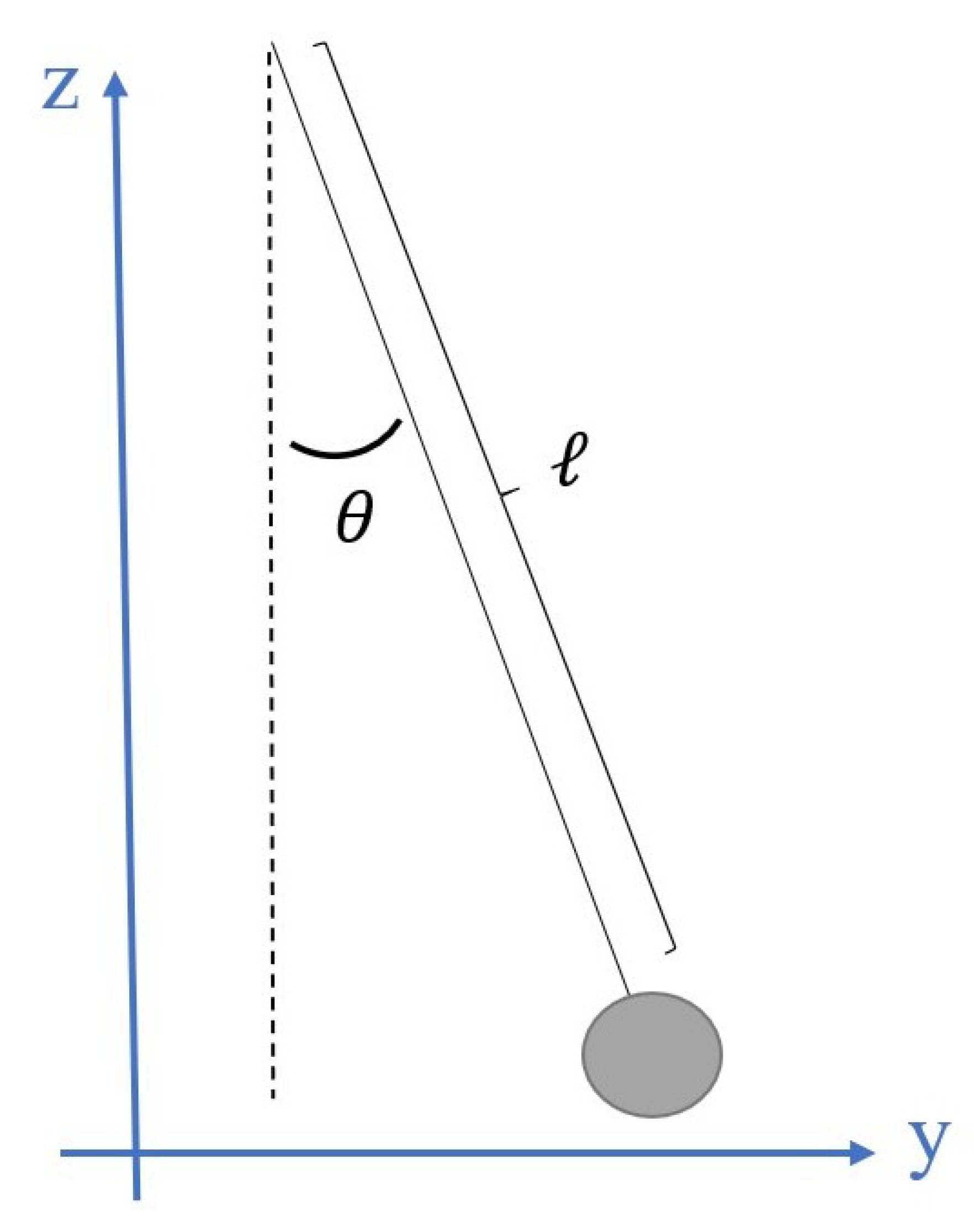
3.1. Simple Pendulum

In this section, we study a simple pendulum on Earth’s surface in the presence of Lorentz violation, in particular the Lorentz-violating effects, described by Lagrangian (2).

3.1.1. Theory: Period

A convenient coordinate system and basic properties of a simple pendulum are shown in Figure 2. In particular, denotes the length of the pendulum string, θ is the angle that the pendulum makes from the vertical, and m is the mass of the pendulum bob.
In terms of these variables, the Lagrangian takes the form
L = m 2 θ ˙ 2 2 [ ( 1 + 2 c y y ) cos 2 θ + ( 1 + 2 c z z ) sin 2 θ 4 c y z sin θ cos θ ] m g ( cos θ ) .
In this expression, c y y , c z z , and c y z are components of the background tensor c j k with respect to a coordinate system attached to Earth’s surface. Since Earth’s surface rotates, they are not truly constant. However, their variation is very slow compared to that of angle θ and so we can regard them as constants as we calculate and solve the pendulum’s equation of motion. More precisely: A typical human-scale pendulum has a period of about 1 s while the Lorentz-violation coefficients c j k vary with a period of order of 24 h, so any errors we make in assuming them to be constant are suppressed by roughly 1 sec 24 hr 10 5 . Note that this reasoning only applies during any particular data-gathering session of the pendulum swinging through a dozen cycles or so. When we compare sessions that are separated by hours, we need to take time variation of c j k into account. In fact, this variation is the key to separating Lorentz-violating effects from conventional effects.
Applying the Euler–Lagrange equations gives the equation of motion, a nonlinear 2nd-order differential equation for θ as a function of time t:
θ ¨ = g sin θ 1 2 c y y cos 2 θ 2 c z z sin 2 θ + 4 c y z sin θ cos θ + θ ˙ 2 2 c y y sin θ cos θ 2 c z z sin θ cos θ + 2 c y z ( cos 2 θ sin 2 θ ) .
Using the usual small-angle approximation, that is, keeping only first order in θ (so sin θ θ and cos θ 1 ), Equation (8) takes the simpler, linear form
θ ¨ = g ( 1 2 c y y ) θ .
This has the general solution
θ ( t ) = θ 0 cos ( ω t + ϕ 0 ) ,
where θ 0 is the amplitude, ϕ 0 is an initial phase, and the angular frequency ω = g ( 1 2 c y y ) . Note that this reduces to the conventional angular frequency when c j k = 0 .
The physical quantity that we directly measured was the period T = 2 π ω . Using the binomial approximation, the period in the presence of Lorentz violation can be written
T = 2 π g ( 1 + c y y )
to first order in c j k . Note again that this reduces to the conventional period when c j k = 0 .
The SME coefficient c y y is a component of a tensor with respect to a coordinate system x , y , z that rotates with Earth, and thus changes as the Earth rotates. In order to clarify the time dependence of c y y , we change coordinates to a non-rotating frame X , Y , Z , seen in Figure 3, commonly used in studies of Lorentz violation [7,8,17]. Using the rotation matrix described in [8], the time dependence of c y y and the period T can be explicitly written
c y y = c X X sin 2 Ω t 2 c X Y cos Ω t sin Ω t + c Y Y cos 2 Ω t , T = 2 π g 1 + c X X sin 2 Ω t 2 c X Y cos Ω t sin Ω t + c Y Y cos 2 Ω t .
In these expressions, Ω denotes the Earth’s sidereal rotation frequency, Ω = 2 π 23 h 56 min . The Lorentz-violation coefficients c J K on the right-hand side of this expression are defined with respect to the nonrotating coordinates X , Y , and Z. It is sometimes useful to write these in the alternate forms
c y y = 1 2 ( c X X + c Y Y ) 1 2 ( c X X c Y Y ) cos 2 Ω t c X Y sin Ω 2 t , T = 2 π g 1 + 1 2 ( c X X + c Y Y ) 1 2 ( c X X c Y Y ) cos 2 Ω t c X Y sin 2 Ω t .
In each of these forms, the last two terms vary at twice Earth’s sidereal frequency while the other(s) are constant.
Note that this transformation assumes that the Earth-frame y points due East. If a pendulum is oriented to swing along a different direction, then the transformation would need to be modified. This causes the period to display two new complications to its behavior: (1) The period has terms that vary at (one times) the sidereal frequency in addition to terms that are constant or vary at twice the sidereal frequency. (2) The period depends on the colatitude χ of the pendulum’s location. For example, the period of a pendulum that swings along the North–South direction takes the form
T = 2 π g 1 + 1 2 ( c X X + c Y Y ) cos 2 χ + c Z Z sin 2 χ 2 c X Z cos χ sin χ cos Ω t 2 c Y Z cos χ sin χ sin Ω t + 1 2 ( c X X c Y Y ) cos 2 χ cos 2 Ω t + c X Y cos 2 χ sin 2 Ω t .
The period of a pendulum that swings in any other direction will have a time dependence that is a linear combination of expressions (13) and (14). The experiments we describe in later sections all used pendulums oriented to swing East–West.

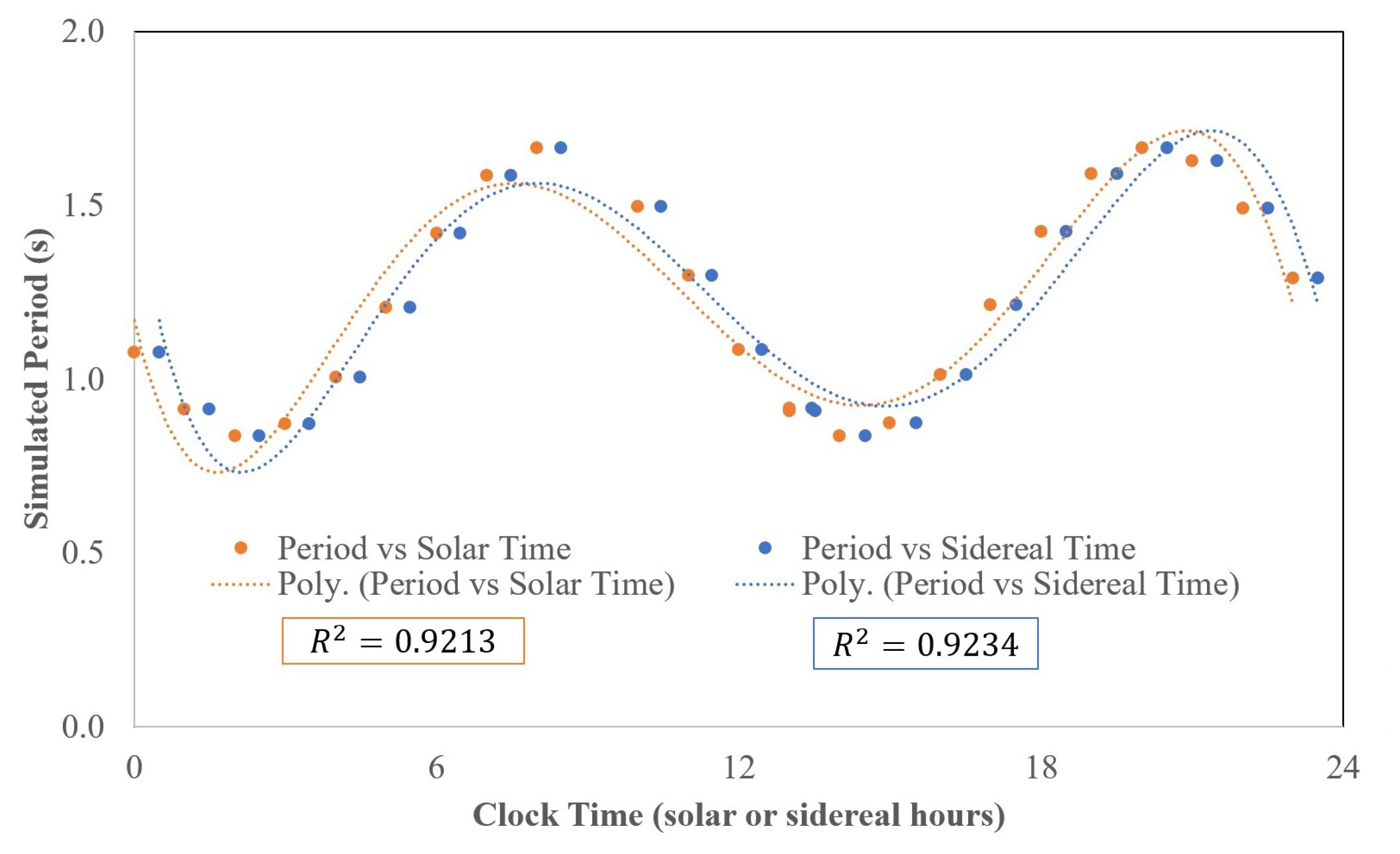
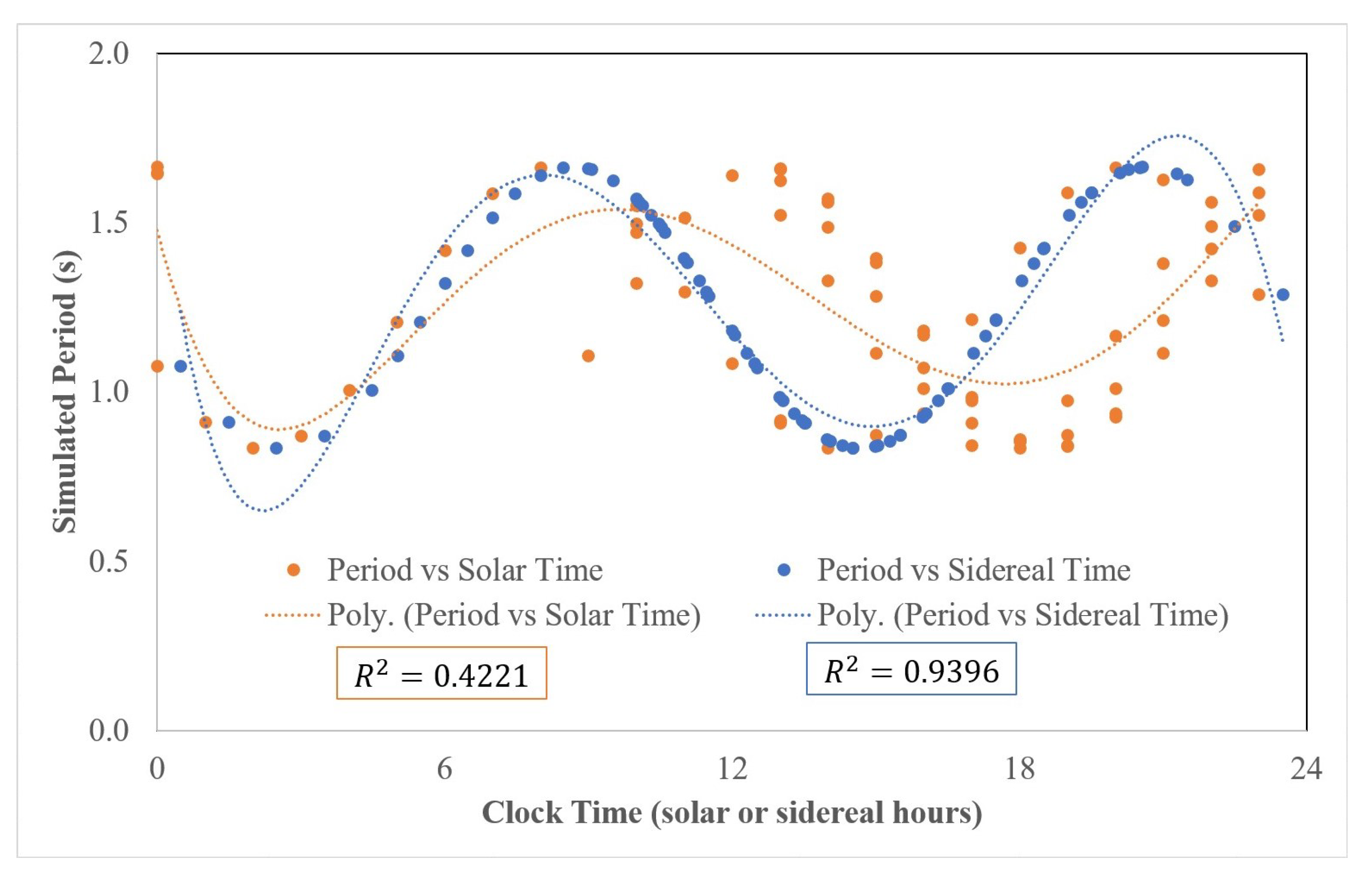
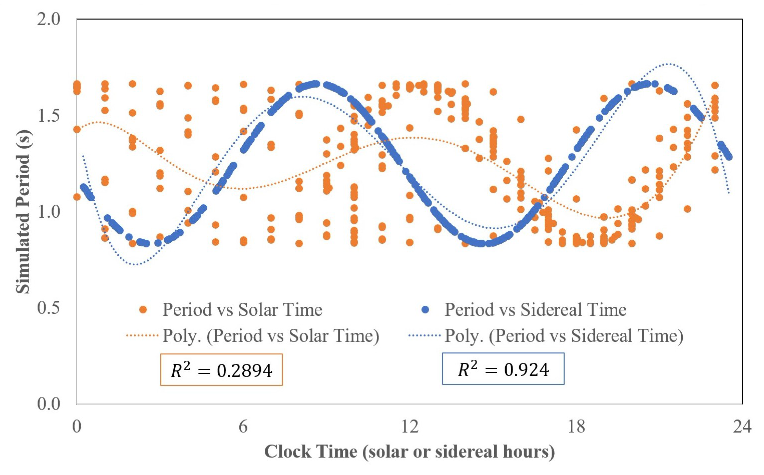
3.1.2. Simulated Data

We collected data for pendulum periods over a span of about 6 months. Before analyzing those data, though, we show some simulated data to help clarify what our experimental signal might look like. This exercise also helps clarify the importance of distinguishing between solar time and sidereal time.
Figure 4, Figure 5 and Figure 6 show simulated data generated under the assumption that c j k is rather large: c X X = 0.32 , c Y Y = 0.18 , and c X Y = 0.41 . In Figure 4, the simulated periods over one day are plotted against solar clock-time (orange) and sidereal clock-time (blue). The data were fit to a 6th-order polynomial and the corresponding R 2 values of the best-fit lines are shown. Figure 5 was similarly plotted but with data simulated over a three-month period. Finally, Figure 6 contains simulated data spanning six months.
As is apparent in Figure 4, it is difficult to distinguish solar variation from sidereal variation with data that span only a single day. The best-fit polynomials have approximately the same R 2 values. Figure 5 and Figure 6 show that data spanning several months allow solar and sidereal to be easily distinguished. In the case of our simulated Lorentz violation, the R 2 values for best-fit curves stay about the same for sidereal variation while they get much worse for solar variation. (The 6-month graph still has hints of a solar-day signal; this is because a large fraction of the data was taken in a single month.) Thus, to accurately measure Lorentz violation, it is important to utilize sidereal time.
A complementary situation occurs in some very high-precision experiments, such as those involving atomic clocks (e.g., [18]) or trapped electrons (e.g., [19]). These experiments may be sensitive to tiny mundane effects that are correlated with the solar day. For example, the lab’s temperature might be slightly warmer during the day and cooler at night (due to, say, humans being present more during the day); this could cause tiny shifts in clock frequencies. In an experiment measuring the anomaly frequency of a single magnetically trapped electron at the University of Washington [19], the data showed small “bumps” whenever the electric trolley outside came near the building [20]. Effects caused by human behavior tend to be more common during daytime, and therefore tend to be correlated with solar time. Valid Lorentz-violating effects may be untangled from mundane effects by searching specifically for variations correlated with sidereal time.

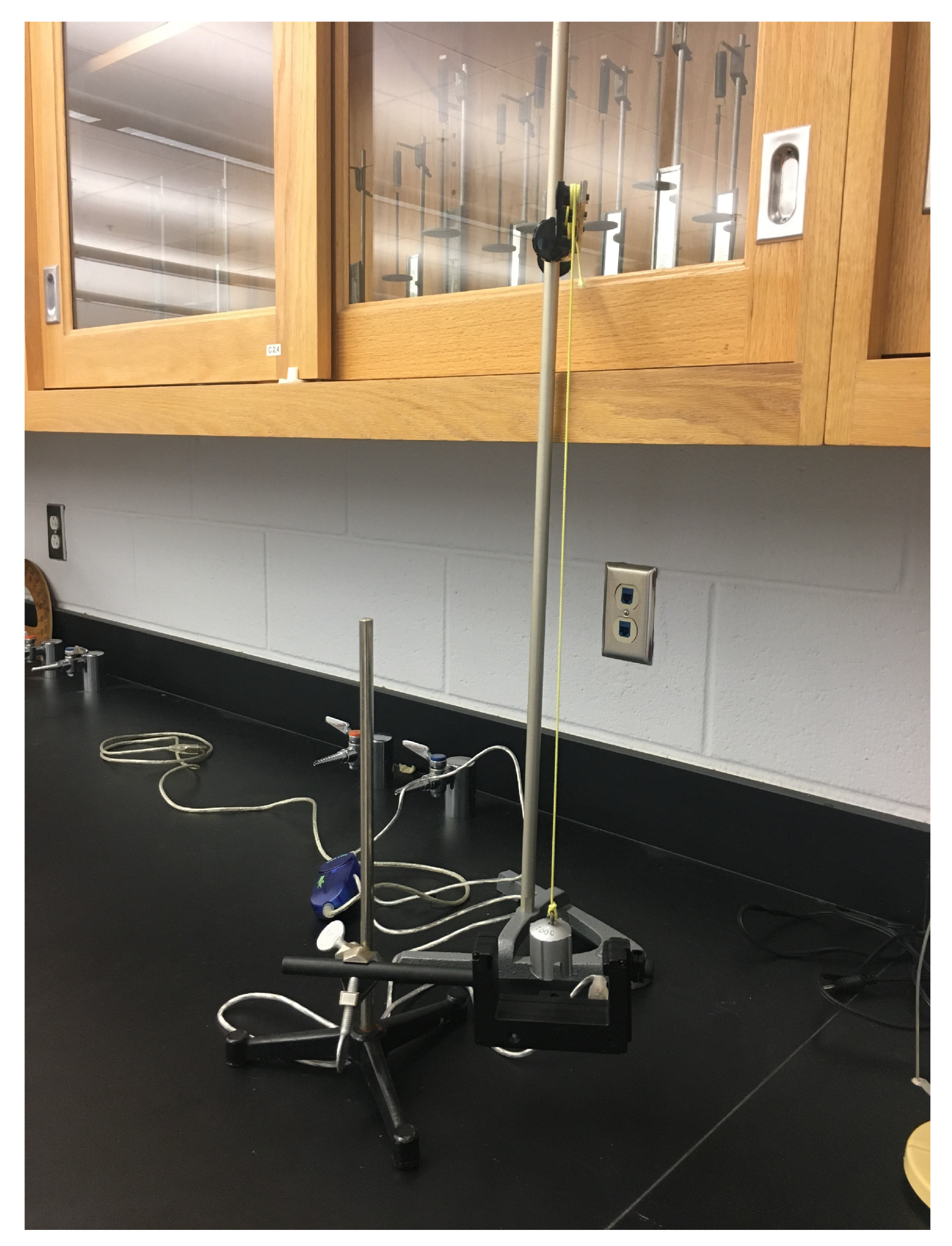
3.1.3. Pendulum Experiment

We built and studied several pendulums, such as the one shown in Figure 7, over approximately a six-month period to search for any Lorentz violation correlated with rotation of Earth. These pendulums were placed across the United States (five in Georgia, one in California) and monitored by multiple experimentalists (as listed in our Acknowledgments). The pendulums’ construction differed slightly, though all were set up to swing along an East–West direction.
The example pendulum seen in Figure 7 was assembled at Berry College using a steel support stand to hold a string with a suspended 100-gram pendulum bob. Other properties of this particular pendulum can be found in Table 1. A PASCO photogate [21] was also attached to a steel support stand and assembled underneath the pendulum so that the pendulum bob swung between the detector ports in order to measure the period of each oscillation. The PASCO photogate gave precision up to 0.0015 s.
On multiple days over a six-month time period, beginning in February 2020 and ending in July 2020, trials were run for twenty-four hours taking the period of the pendulum at the beginning of each hour. For each measurement, the pendulum would be brought to an initial angle from the vertical, as seen in Table 1, and released to oscillate fifteen times. The photogate calculated the period of each oscillation and so the average over fifteen oscillations was used to reduce any error caused by the pendulum being misaligned with or hitting the photogate. To further reduce this systematic error, the average period over fifteen oscillations was repeated three times for each trial. These three periods were then averaged to determine the approximate period of the pendulum at the beginning of each hour.
This process was repeated for each trial until reaching the twenty-four hour period from the day before, and then continued on another date the next month. All period measurements were recorded along with the date and time of the measurement. Then, for each measurement, the corresponding Solar and Sidereal times were calculated using Equation (1) based on a start date of the vernal equinox in the year 2000 (20 March 2000), which is the base time for standard Sun-centered coordinates. This start date ensured that our measured coefficients c J K in the Sun frame were the same as those measured in past Lorentz-violation studies.
Different pendulum setups had slightly different lengths, and therefore conventional physics predicts that they will have slightly different periods. To allow us to combine their data, therefore, we introduced a normalized period, defined to be each period measurement divided by the conventional period for that setup:
Normalized period = T ( t ) 2 π / g = 1 + c X X sin 2 Ω t 2 c X Y cos Ω t sin Ω t + c Y Y cos 2 Ω t .
This quantity is the same for all setups.
We used multiple linear regression to determine the SME coefficients and seek evidence of Lorentz symmetry violation. However, as evident in Equations (12), (13), and (15), the period is not a linear function of time but rather a sinusoidal function of time. Thus, we used sinusoidals corresponding to each SME coefficient in Equation (15) as our independent variables x j
x 1 = sin 2 Ω t x 2 = cos 2 Ω t x 3 = 2 sin Ω t cos Ω t ,
with dependent variable c y y = x 1 c X X + x 2 c Y Y + x 3 c X Y = normalized period   1 . Using the method of least squares function in Excel (LINEST), the SME coefficients were calculated using all of the period data over a six month interval and multiple pendulum setups. The results and their uncertainties can be found in Table 2.
Each of these is consistent with zero at the level of about 10 3 .
It should be noted that these bounds are several orders of magnitude stronger than would have been achieved by directly comparing each measurement of the period with the value predicted by conventional physics. This is typical in studies of Lorentz violation—sensitivity to sidereal effects is generally much stronger than sensitivity in absolute measurements. This is part of the reason that searches for Lorentz violation in low-energy, high-precision experiments could potentially detect Planck-scale effects in theories of physics beyond the Standard Model.
The values of c J K for different substances may a priori be unequal. For our experiment, the relevant values of c J K are those for our pendulum bobs, c J K bob . Typically, studies of the SME refer to values of c J K for protons, neutrons, and electrons, c J K p , c J K n , and c J K e , respectively. We may approximately relate our bounds to these as follows: the effective value of c J K for a composite object is an average of the values for its constituent particles, weighted by mass. Typical solid materials have roughly the same number of protons, neutrons, and electrons; proton and neutron masses are roughly equal, while the electron mass is about 1/2000 of each. Therefore, our c J K is approximately given by
c J K bob 1 2 c J K p + 1 2 c J K n + 1 2000 c J K e .
From this, we conclude that we have bounded c X X , c X Y , and c Y Y for protons and neutrons at the level of 10 3 and for electrons at the level of 10 0 . These are far away from the bounds that have been achieved in high-precision atomic experiments [7], which place bounds on c J K for protons and neutrons at the level of 10 30 and for electrons at the level of 10 27 . This is fine, as our experiment is not intended to be competitive with modern experiments. Rather, it is intended to serve as an illustration of the concepts and methods that appear in studies of Lorentz violation while being accessible to typical undergraduate students.

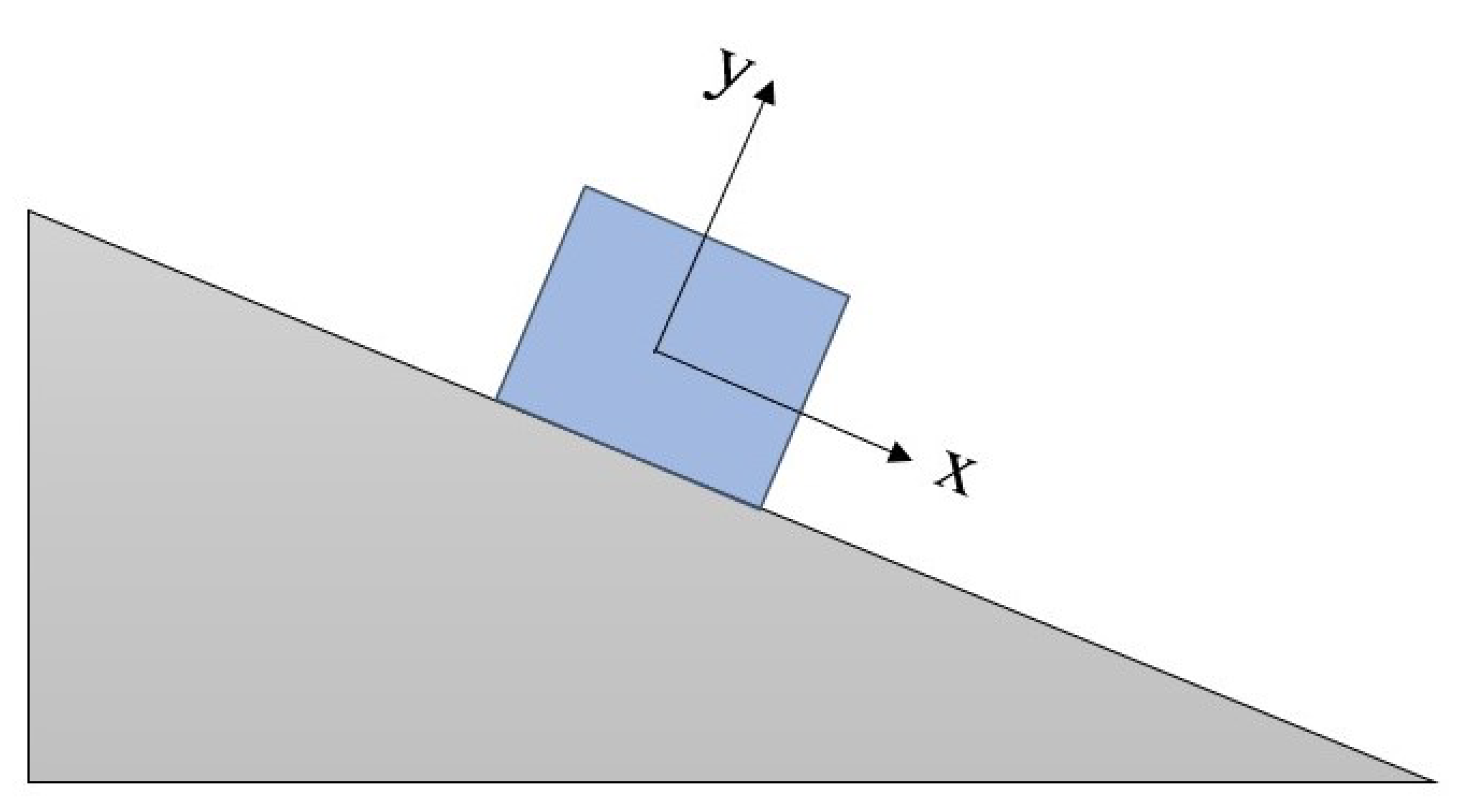
3.2. Block on Inclined Plane

In this section, we consider some aspects of a block on a frictionless inclined place on Earth’s surface in the presence of a Lorentz violation, in particular the Lorentz-violating effects described by Lagrangian (2). This system has already been analyzed in [15]; we briefly summarize their findings and then add a few comments.
A standard set of coordinates for analyzing a block-on-plane system is shown in Figure 8, with the x axis pointing parallel down the plane and the y axis pointing perpendicular to and out of the plane. As in Ref. [15], we restrict attention to the case where c j k , and hence the effective mass matrix m j k , are diagonal in our chosen coordinate system. To first order in c j k , they found the acceleration down the ramp to be
a x = ( 1 2 c x x ) g sin θ .
The gravitational force on the block is
F g = m g sin θ x ^ m g cos θ y ^ ;
recall that the gravitational force in this model is conventional, involving the (scalar) gravitational mass m. Since we are neglecting friction, the only other force acting on the block is the normal force, which, by definition, is perpendicular to the plane:
F N = F N y ^ .
Now consider the x components of all of these. The x component of the net force is m g sin θ while the x component of the acceleration is ( 1 2 c x x ) g sin θ : The net force and the acceleration are not parallel to each other.
On the other hand, the effective mass matrix times the acceleration is
m j k a k = m 1 + 2 c x x 0 0 0 1 + 2 c y y 0 0 0 1 + 2 c z z ( 1 2 c x x ) g sin θ 0 0 = m g sin θ 0 0
to first order in c j k . Therefore, the Lorentz-violating Newton’s 2nd Law (5) successfully relates net force and acceleration for this system while the conventional Newton’s 2nd Law fails.

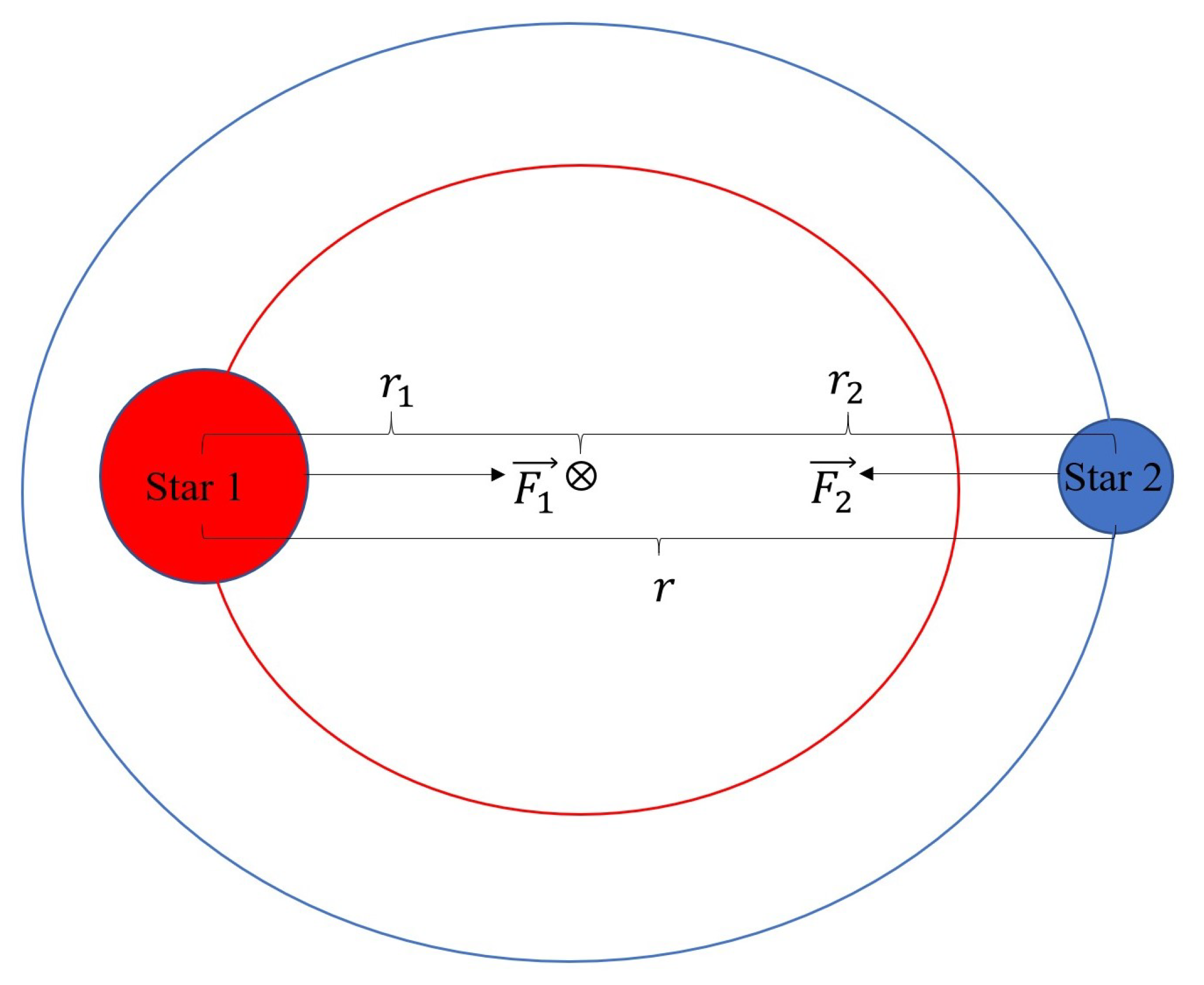
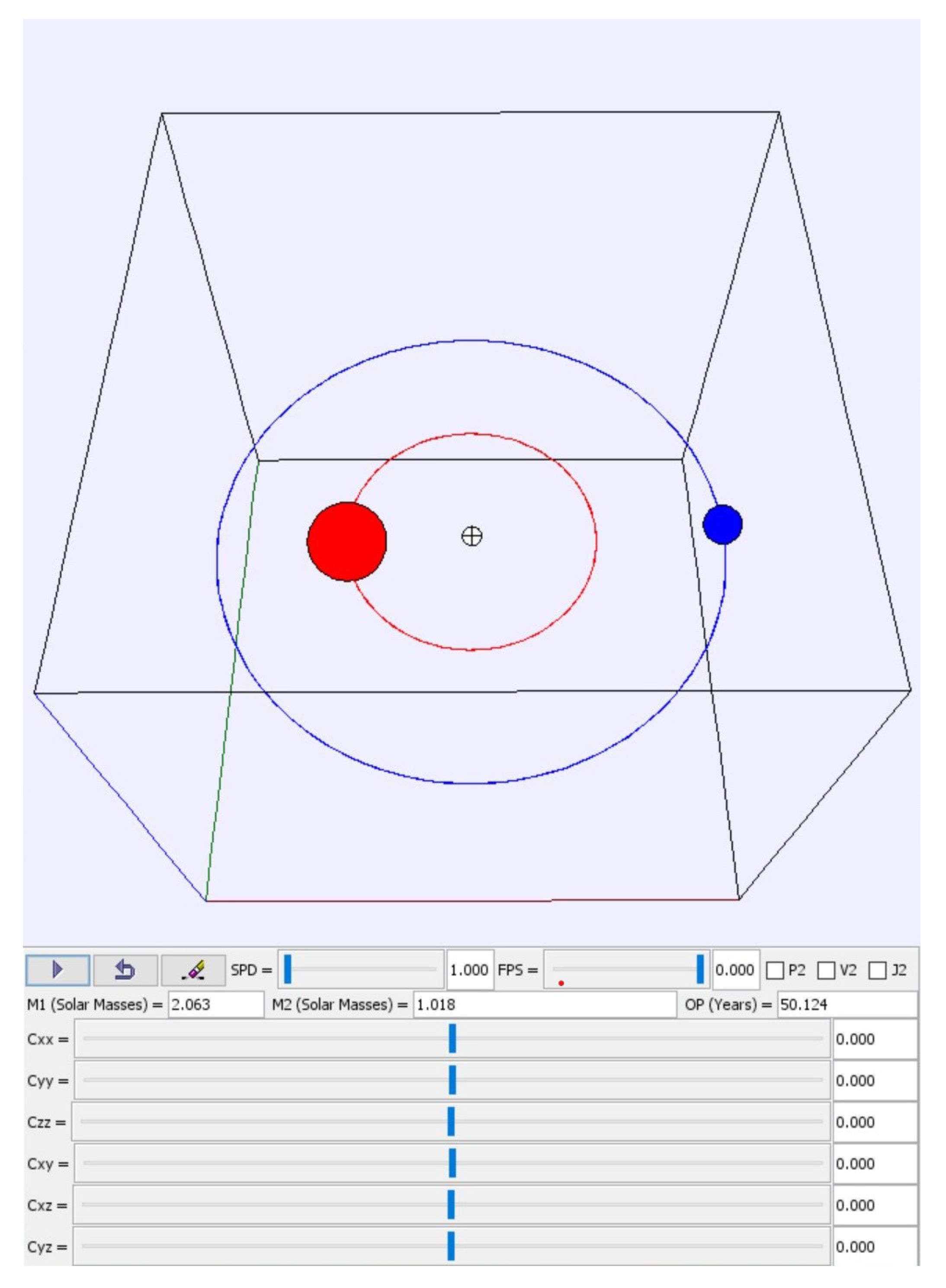
3.3. Binary Star System

The final system we use to study SME Lorentz-violating effects is a binary star system. In this system, a detached star system was considered with two stars orbiting about a common center of mass.
We first define some variables and derive the key theoretical expressions for this system. A few ideas are illustrated with data from a numerical simulation. We then describe the simulation in more detail and describe some interesting behavior that may be observed in it. Our completed simulation may be downloaded from the Open Source Physics group [22].

3.3.1. Theory: Equations of Motion

Neglecting all other relativistic and gravitational forces, the only forces acting on the stars are the gravitational forces that they exert on each other (as seen in Figure 9).
In our model of Lorentz violation, Newton’s 3rd Law holds and Newton’s law of universal gravitation is conventional. Thus, the gravitational force on Star 1 will be equal in magnitude and opposite in direction to the gravitational force on Star 2. Newton’s law of universal gravitation produces the following forces for the x, y, and z components of Star 1 and Star 2
F x 1 = G m 1 m 2 r 3 ( x 2 x 1 ) = F x 2 , F y 1 = G m 1 m 2 r 3 ( y 2 y 1 ) = F y 2 , and F z 1 = G m 1 m 2 r 3 ( z 2 z 1 ) = F z 2 ,
where G = 4 π 2 AU 3 /M years 2 is the gravitational constant in astronomical units, r = ( x 2 x 1 ) 2 + ( y 2 y 1 ) 2 + ( z 2 z 1 ) 2 is the distance between the two stars in AU, and m 1 and m 2 are the masses of Star 1 and Star 2 in solar masses, respectively.
Next, Newton’s second law, Equation (5), was used to determine the components of the acceleration of the two stars, including Lorentz-symmetry-violating effects and keeping only first-order terms in c j k . This produced the following accelerations of the two stars:
a 1 = G m 2 r 3 q 1 x x ^ + q 1 y y ^ + q 1 z z ^ , a n d a 2 = G m 1 r 3 q 2 x x ^ + q 2 y y ^ + q 2 z z ^ ,
where
q 1 x = ( 1 2 c x x ) ( x 2 x 1 ) 2 c x y ( y 2 y 1 ) 2 c x z ( z 2 z 1 ) = q 2 x , q 1 y = 2 c x y ( x 2 x 1 ) + ( 1 2 c y y ) ( y 2 y 1 ) 2 c y z ( z 2 z 1 ) = q 2 y , a n d q 1 z = 2 c z x ( x 2 x 1 ) 2 c z y ( y 2 y 1 ) + ( 1 2 c z z ) ( z 2 z 1 ) = q 2 z .

3.3.2. Theory: Energy

The total energy of the binary star system may be found by simply adding the potential and kinetic energy, where the potential energy is conventional
U = G m 1 m 2 r ,
and the kinetic energy formula is modified by Lorentz violation
K = 1 2 v 1 j m 1 j k v 1 k + 1 2 v 2 j m 2 j k v 2 k .
Explicitly calculating the kinetic energy of each star, for star 1
K 1 = m 1 2 ( 1 + 2 c x x ) v 1 x 2 + ( 1 + 2 c y y ) v 1 y 2 + ( 1 + 2 c z z ) v 1 z 2 + 4 c x y v 1 x v 1 y + 4 c x z v 1 x v 1 z + 4 c y z v 1 y v 1 z ,
and for star 2,
K 2 = m 2 2 ( 1 + 2 c x x ) v 2 x 2 + ( 1 + 2 c y y ) v 2 y 2 + ( 1 + 2 c z z ) v 2 z 2 + 4 c x y v 2 x v 2 y + 4 c x z v 2 x v 2 z + 4 c y z v 2 y v 2 z .
Thus, the total energy of the binary star system can be written as
E = K 1 + K 2 + U .
Since the Lagrangian (2) has no explicit time dependence, this energy is conserved.

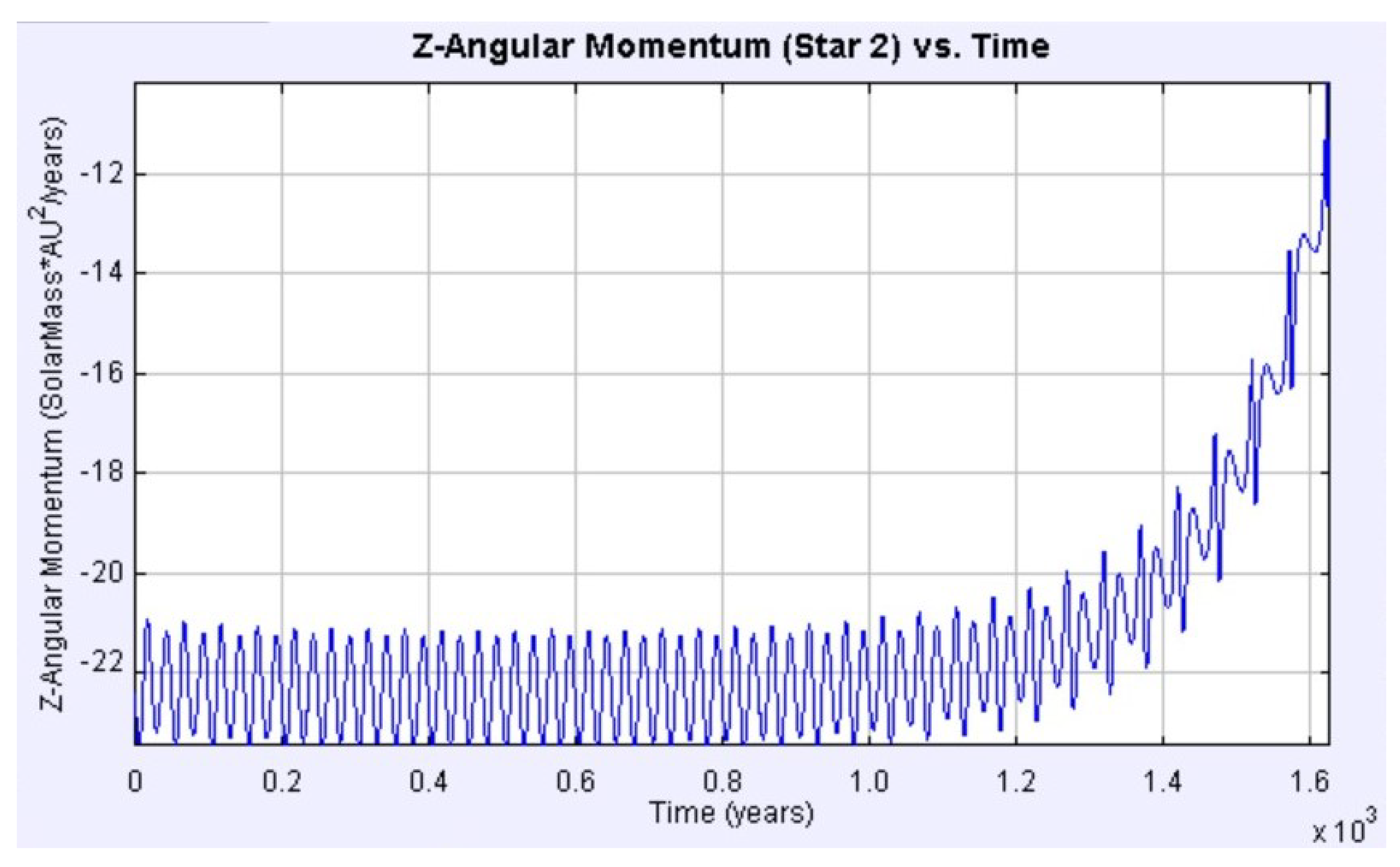
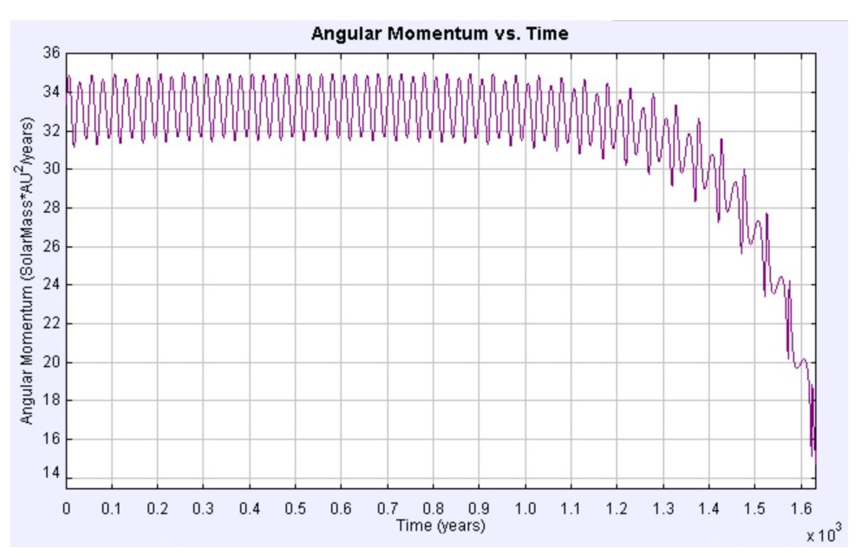
3.3.3. Theory: Angular Momentum

In order to study angular momentum conservation for the Lorentz-symmetry-violating binary star system, we may calculate the rate of change of angular momentum. The momentum of one of the stars is equal to
p j = m j k v k ,
where m j k is the mass matrix in Equation (6) and v k is the translational velocity vector of the star. In terms of the momentum and the star’s position r , the angular momentum can be written J = r × p or
J j = ε j k r k p ,
where ε j k is the Levi-Cevita antisymmetric tensor.
The rate of change of the angular momentum follows from the product rule
d J j d t = ε j k d r k d t p + r k d p d t .
The time derivative of the momentum may be expressed as the net force by using the Lorentz-violating Newton’s Second Law in Equation (5)
d p d t = m k a k = F ,
where a k is the acceleration of the star and F is the net force vector acting on it. Thus, we can rewrite Equation (32) using Equation (33)
d J j d t = ε j k d r k d t p + r k F .
Notice that in Figure 9 the net force on each star is simply the gravitational force from the other star. In our model, the gravitational force is conventional, and is thus antiparallel to the radial vector. Therefore, r × F = 0 and we can rewrite Equation (32) as
d J d t = v × p .
An important thing to notice is the fact that in this situation, the velocity is no longer parallel to the momentum. This can be seen in Figure 10, a screenshot from the simulation illustrating the Lorentz-symmetry-violating effect to binary star systems, where the gray vector is the velocity and the black vector is the momentum. This is meaningful if the c j k values become non-negligible, and thus the effective mass matrix alters the direction of the momentum.
Therefore, since the momentum and velocity are no longer parallel, it can be concluded that the total angular momentum of the system is no longer conserved. For example, the z-component of the angular momentum is plotted in Figure 11 to simulate the Lorentz-symmetry-violating effects for one of the individual stars. As Figure 12 shows, the angular momentum changes are not simply the precession of the orbit, as the magnitude of angular momentum decreases.

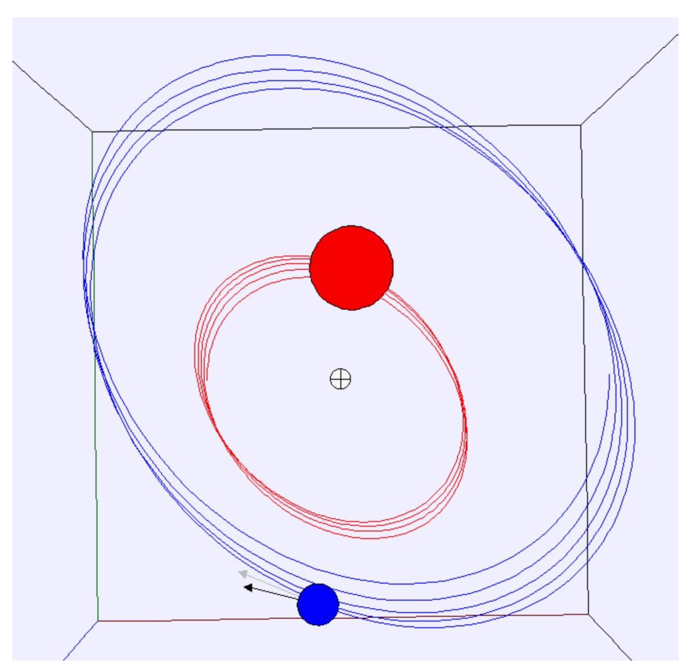
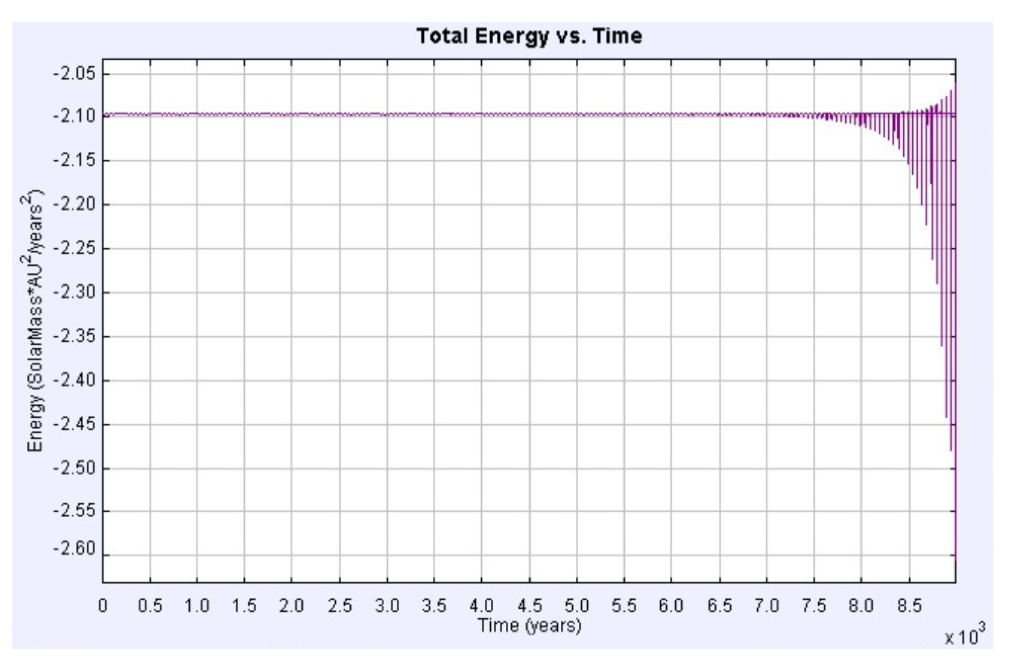
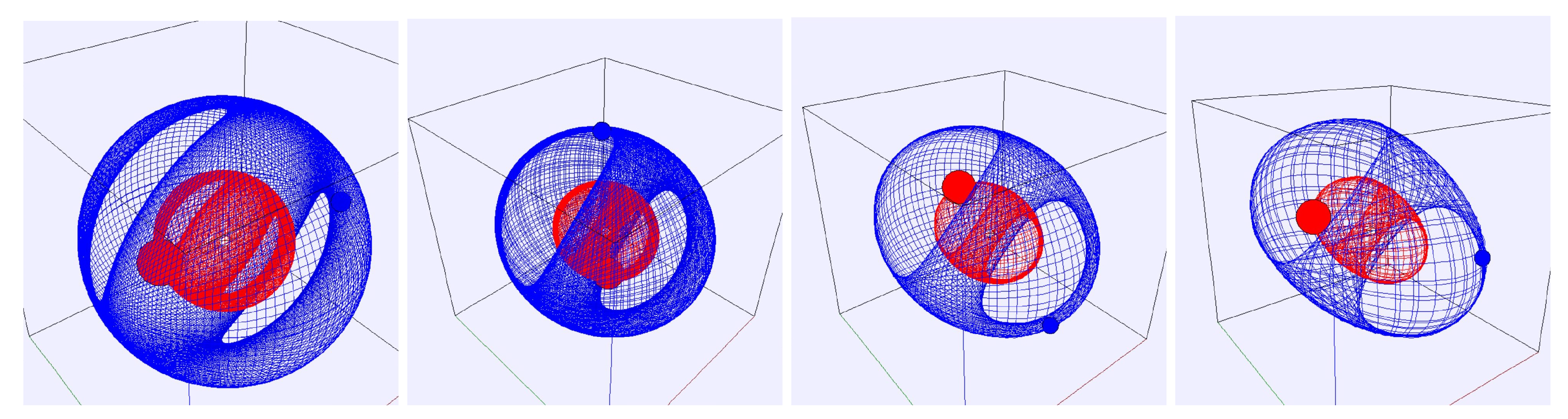
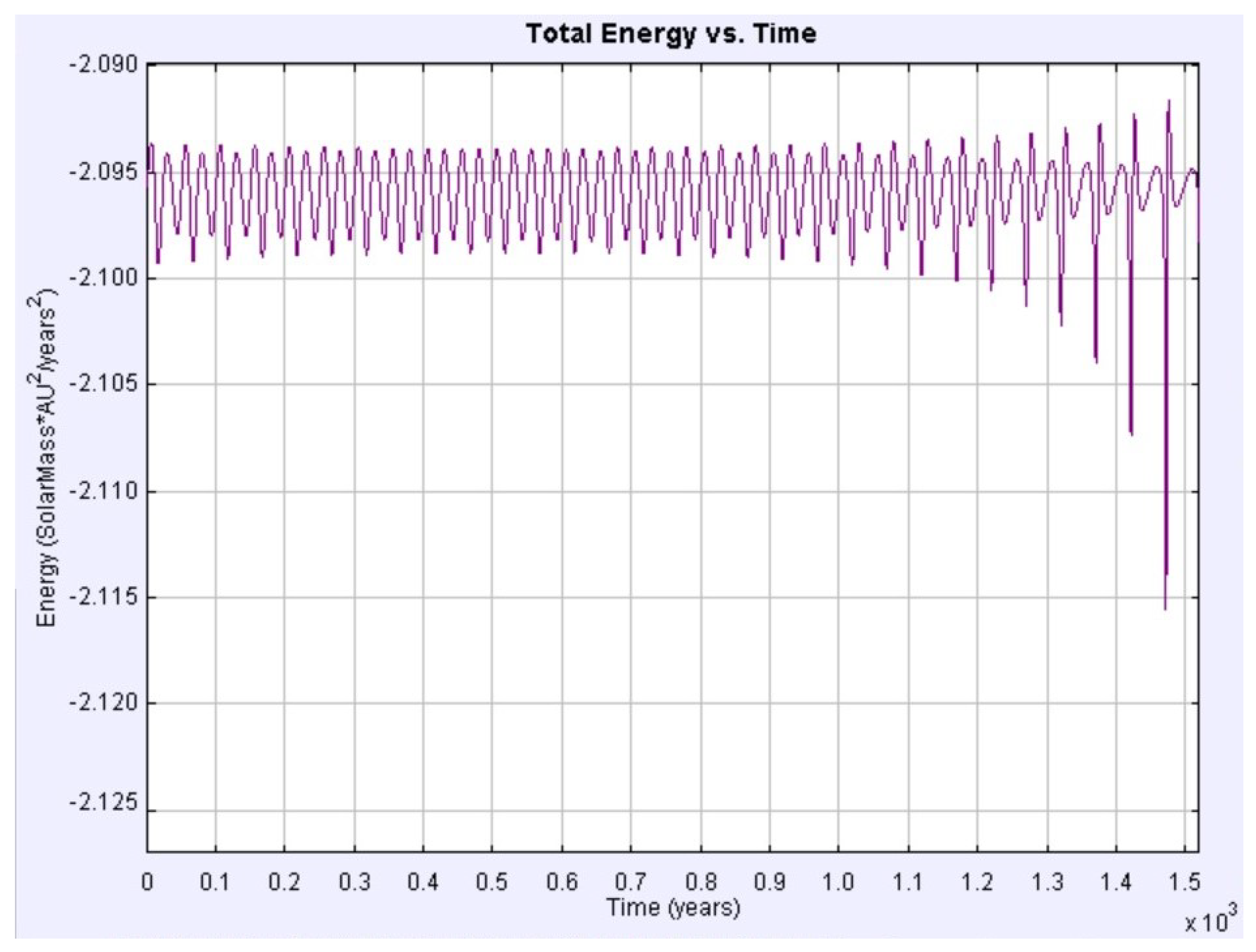
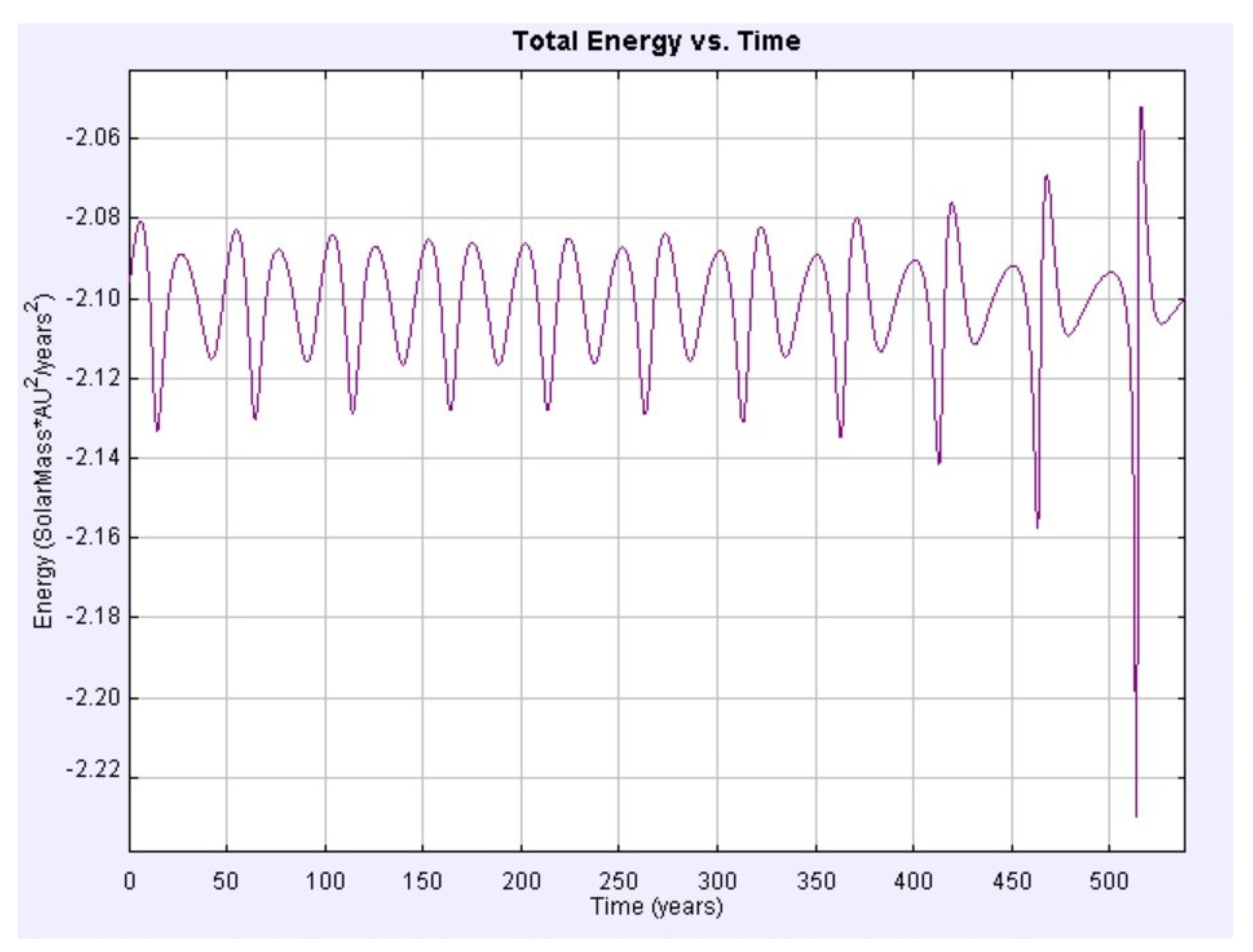
3.3.4. Binary Star System Computational Simulation

To study the Lorentz violation effects on binary stars, an Easy Java Simulation (EJS) was created to simulate any 3D detached binary system and the effects of the background tensor fields on the motion of the stars [22]. EJS uses embedded Java and Javascript programming. Throughout this section, all masses are stated as multiples of our Sun’s mass M , distances are stated as multiples of average Earth–Sun separation AU, and times are stated as multiples of Earth years.
Our simulation specifically uses data for the closest binary star system to Earth, Sirius A and B. We sometimes label Sirius A as “Star 1” and it is colored red in the simulation. Similarly, we sometimes label Sirius B as “Star 2” and it is colored blue. The orbit parameters and initial conditions of these stars can be found in Table 3.
Kepler’s third law of planetary motion may be used to determine relationships between several of these quantities. For example,
m 1 + m 2 = r 3 ( τ o p ) 2
relates τ o p , the orbital period of the binary star system, and r, the stars’ initial separation. If the system’s center of mass is located at ( 0 , 0 , 0 ) , then the masses and initial positions of the stars must be related by
m 1 r 1 = m 2 r 2 ,
where r 1 and r 2 are the distances from the center of mass to Star 1 and Star 2, respectively. Using Equations (36) and (37), the positions were found such that Star 1 was located initially at ( r 1 , 0 , 0 ) and Star 2 at ( r 2 , 0 , 0 ) .
Since the initial orbits are roughly circular, the initial velocity of Star 1 may be written in terms of its orbital period as
v y 1 2 π r 1 τ o p .
The initial value of v y 2 may be determined by working in a reference frame in which the total initial momentum of the system is zero. Since the SME momentum p j = m ( δ j k + 2 c j k ) v k is a linear function of Newtonian momentum m v j , this condition may be written as requiring that the initial Newtonian momentum also be zero: m 1 × v 1 = m 2 × v 2 . Recall that momentum is conserved in the Lorentz-violating SME, so the system will continue to have a total momentum of zero. Once inputting these initial conditions, as well as the equations of motion, the Velocity Verlet algorithm was used to solve the three-dimensional differential equations in Equation (23) to produce the subsequent trajectories of the stars.
The user interface is shown in Figure 13. The user has the ability to change the mass of both or either of the stars in order to visualize the effects on the orbit of the binary stars. Similarly, the orbital period can be altered in order to change the initial conditions of the simulation. Increasing the orbital period will increase the initial separation of the stars, and will decrease v y 1 and ultimately change the value of v y 2 as well. This gives the user the ability to observe the motion of a variety of different binary star systems that could possibly exist in our universe. Finally, the default EJS starts with all SME coefficients set to zero, but their values can be altered with the accompanying sliders to view the effects of Lorentz symmetry violation on the motion of binary stars.
We can use the simulation to verify some theoretical ideas we discussed earlier. For example, using Equation (29), the total energy may be plotted in the simulation to check energy conservation. Sample data are shown in Figure 14, where it may be seen that the energy is not strictly constant. This appears to be a numerical artifact. The rough outline of our reasoning for this claim is as follows: first, numerical simulations do not calculate exact values of anything so some apparent variation is normal. Moreover, our derivation of the equation of motion neglected terms that are quadratic in c j k . If some c j k 0.1 , that means we are neglecting effects at the level of c j k 2 1 % . An energy that varies in the simulation by a few percent is therefore consistent with energy conservation.
We may expand this argument with more details. First, for most values of c j k , the orbits are stable (such as in Figure 15, where a variety of long-term trajectories are shown) and the apparent energy non-conservation is a numerical artifact. For example, with c x z = 0.07 (and others zero), the total energy varies from 2.082 to 2.102 units, a variation of about 1%. Meanwhile, for the same value of c x z , the z component of angular momentum varies between 0 and 22 units, which is a huge variation. This suggests that the angular-momentum variation is a real effect while the energy variation is a numerical error. Moreover, the system appears to be stable over very long time-scales for most non- zero choices of c j k .
However, for some values of c j k , the energy eventually diverges, as shown in Figure 14. This is also likely to be a numerical artifact, for the following reasoning: In conventional orbital mechanics, a constant energy with an increasing angular momentum corresponds to an increasingly eccentric orbit. The more-eccentric orbit causes the objects to pass very close to each other, e.g., the perihelion gets smaller and smaller. At small values of separation between stars, the gravitational force gets very large. Numerically, the separation gets close to zero, and so the gravitational-force calculation becomes a division by zero (or close to zero), which is a common numerical instability.
This argument may be further supported by the observation that the simulation diverges sooner for larger values of c x y than for smaller values of c x y . For example, when c x y = 0.01 and all other c j k = 0 , the energy breakdown occurs, as seen in Figure 14, after 8500 years. When c x y = 0.05 , the major breakdown occurs after about 1400 years, as seen in Figure 16. For c x y = 0.1 , it occurs between 500 to 700 years, as in Figure 17, and when c x y = 0.2 , the simulation breaks around 300 or 400 years. Therefore, it appears that the breakdown-time is inversely proportional to the size of c x y .
We have considered the following alternate explanation: the conserved energy is K + V. Calculation of the equations of motion involves quantities like ( 1 + c j k ) 1 , which are then approximated to 1 c j k . That is, we neglect higher powers of c j k . It is reasonable to consider that these higher powers might be necessary for energy conservation when c j k is somewhat large (about 0.1 or so). However, this idea does not work. We worked out a model with c x x non-zero and kept all powers of it. When this model is programmed into the numerical simulation, the energy behaved essentially the same as before, i.e., it varied by a few percent. That is, keeping higher powers of c j k did not cause the energy to appear any more conserved.
For non-zero values of c x z and c y z , the simulation seems to be well behaved. It is stable for many, many cycles. In fact, we have not yet found any values of c x z and c y z that lead to instability. Again, in this regime, the energy varies by around 1% while the angular momentum components vary by huge amounts, lending support to the claim that the energy variation is a numerical artifact. We conclude that the apparent energy nonconservation is a numerical artifact rather than a true effect of Lorentz violation.
Additionally, the simulation includes plots of speed of the stars versus time and separation between the stars versus time. In these plots, one can understand how Lorentz-violating effects affect the change in speed and increased separation between the stars.
For many values of c j k , the system seems to be stable for very long time-scales. The trajectory of each star sweeps out a manifold that is a large portion of an ellipsoid, as shown in Figure 15. However, the trajectory manifold does not form a complete ellipsoid. There are regions of the potential ellipsoid where the stars do not go. These mouth-shaped regions occur for a wide variety of values of c j k , and so are not likely to be numerical accidents. Recall that the variation in angular momentum is given by d J / d t = v × p . During an orbit, these flop around a fair bit, and so it is plausible that d J / d t causes a reversal of J z often enough to forbid some values. An analytical understanding of this issue would be interesting but is beyond the scope of this paper.

4. Discussion and Conclusions

The classical limit of the SME may be used to illustrate many facets of Lorentz violation. Bounds on Lorentz violation using a macroscopic pendulum are not competitive with bounds from high-precision atomic experiments, but it still allows exploration of such effects as sidereal variation.
The numerical simulation of a binary star system can greatly aid visualization of Lorentz-violating effects such as non-conservation of angular momentum. Some behavior seen in the simulation is not easily explainable. For example, the “mouths” in trajectory manifolds are intriguing. Future projects that show a clear analytical explanation for their existence, shape, and size would be very interesting, as would an analytical study of the stability of orbits.

Author Contributions

All authors contributed equally. All authors have read and agreed to the published version of the manuscript.

Funding

This research received no external funding.

Acknowledgments

We would like to acknowledge several groups. For aid with performing pendulum measurements, we would like to thank Paolo Francisco, Kimberly Lowndes, Garrett Rowls, Jordan Schoon, Quinn Smith, and Zachary Lindsey. For help with EJS, we would like to thank Todd Timberlake. Finally, for financial support, we would like to thank Berry College.

Conflicts of Interest

The authors declare no conflict of interest.

Abbreviations

The following abbreviations are used in this manuscript:
SMEStandard-Model Extenshion
EJSEasy Java Simulation

References

  1. Kostelecky, V.; Samuel, S. Spontaneous Breaking of Lorentz Symmetry in String Theory. Phys. Rev. D 1989, 39, 683. [Google Scholar] [CrossRef] [PubMed] [Green Version]
  2. Kostelecky, V.; Potting, R. CPT and strings. Nucl. Phys. B 1991, 359, 545–570. [Google Scholar] [CrossRef]
  3. Connes, A. Noncommutative Geometry; Springer: San Diego, CA, USA, 1994. [Google Scholar]
  4. Carroll, S.M.; Harvey, J.A.; Kostelecky, V.A.; Lane, C.D.; Okamoto, T. Noncommutative field theory and Lorentz violation. Phys. Rev. Lett. 2001, 87, 141601. [Google Scholar] [CrossRef] [PubMed] [Green Version]
  5. Colladay, D.; Kostelecky, V. Lorentz violating extension of the standard model. Phys. Rev. D 1998, 58, 116002. [Google Scholar] [CrossRef] [Green Version]
  6. Kostelecky, V. Gravity, Lorentz violation, and the standard model. Phys. Rev. D 2004, 69, 105009. [Google Scholar] [CrossRef] [Green Version]
  7. Kostelecký, V.A.; Russell, N. Data Tables for Lorentz and CPT Violation. Rev. Mod. Phys. 2011, 83, 11–31. [Google Scholar] [CrossRef] [Green Version]
  8. Kostelecky, V.A.; Lane, C.D. Constraints on Lorentz violation from clock comparison experiments. Phys. Rev. 1999, D60, 116010. [Google Scholar] [CrossRef] [Green Version]
  9. Kostelecký, V.A.; Vargas, A.J. Lorentz and CPT Tests with Clock-Comparison Experiments. Phys. Rev. D 2018, 98, 036003. [Google Scholar] [CrossRef] [Green Version]
  10. Safronova, M.; Budker, D.; De Mille, D.; Kimball, D.F.J.; Derevianko, A.; Clark, C. Search for New Physics with Atoms and Molecules. Rev. Mod. Phys. 2018, 90, 025008. [Google Scholar] [CrossRef] [Green Version]
  11. Lane, C.D. Using Comparisons of Clock Frequencies and Sidereal Variation to Probe Lorentz Violation. Symmetry 2017, 9, 245. [Google Scholar] [CrossRef] [Green Version]
  12. Bailey, Q.G.; Kostelecky, V. Signals for Lorentz violation in post-Newtonian gravity. Phys. Rev. D 2006, 74, 045001. [Google Scholar] [CrossRef] [Green Version]
  13. Kostelecky, A.V.; Tasson, J.D. Matter-gravity couplings and Lorentz violation. Phys. Rev. D 2011, 83, 016013. [Google Scholar] [CrossRef] [Green Version]
  14. Kostelecky, A.V.; Russell, N. Classical kinematics for Lorentz violation. Phys. Lett. B 2010, 693, 443–447. [Google Scholar] [CrossRef] [Green Version]
  15. Bertschinger, T.; Flowers, N.A.; Moseley, S.; Pfeifer, C.R.; Tasson, J.D.; Yang, S. Spacetime Symmetries and Classical Mechanics. Symmetry 2018, 11, 22. [Google Scholar] [CrossRef] [Green Version]
  16. Jansky, K.G. Electrical Disturbances Apparently of Extraterrestrial Origin. Proc. Inst. Radio Eng. 1982, 21, 1387–1398. [Google Scholar]
  17. Kostelecky, V.; Mewes, M. Signals for Lorentz violation in electrodynamics. Phys. Rev. D 2002, 66, 056005. [Google Scholar] [CrossRef] [Green Version]
  18. Pihan-Le Bars, H.; Guerlin, C.; Lasseri, R.; Ebran, J.; Bailey, Q.; Bize, S.; Khan, E.; Wolf, P. Lorentz-symmetry test at Planck-scale suppression with nucleons in a spin-polarized 133Cs cold atom clock. Phys. Rev. D 2017, 95, 075026. [Google Scholar] [CrossRef] [Green Version]
  19. Mittleman, R.; Ioannou, I.; Dehmelt, H.; Russell, N. Bound on CPT and Lorentz symmetry with a trapped electron. Phys. Rev. Lett. 1999, 83, 2116–2119. [Google Scholar] [CrossRef]
  20. Mittleman, R.K.; (University of Washington, Seattle, WA, USA). Personal communication, 1999.
  21. PASCO Smart Gate PS-2180. Available online: www.pasco.com (accessed on 20 February 2020).
  22. Clyburn, M. Binary Star System with Lorentz Symmetry Violating Effects. 2020. Available online: https://www.compadre.org/OSP/items/Detail.cfm?ID=15555 (accessed on 10 September 2020).
Figure 1. Background vector field that violates rotational symmetry. (Image constructed by Charles D. Lane with POV-Ray software. Earth map from http://visibleearth.nasa.gov/).
Symmetry 12 01734 g001
Figure 2. Simple pendulum schematic.
Symmetry 12 01734 g002
Figure 3. Transformation of coordinates [8] between a rotating Earth-based frame x , y , z and a nonrotating Sun-based frame X , Y , Z . The origins of the frames are shown as coinciding to ease understanding of relative directions.
Symmetry 12 01734 g003
Figure 4. Plot of simulated period vs different clock times spanning 1 day.
Symmetry 12 01734 g004
Figure 5. Plot of simulated period vs different clock times spanning 3 months.
Symmetry 12 01734 g005
Figure 6. Plot of simulated period vs different clock times spanning 6 months.
Symmetry 12 01734 g006
Figure 7. Setup of one of the pendulums used to experimentally detect Lorentz symmetry violation.
Symmetry 12 01734 g007
Figure 8. Block on plane coordinate system.
Symmetry 12 01734 g008
Figure 9. Diagram of a binary star system where the only force on Star 1 (red) is the gravitational force from Star 2 (blue) and vice versa. The center of mass is denoted with a “⊗” symbol and all calculations are done in a frame where it is at rest.
Symmetry 12 01734 g009
Figure 10. EJS screenshot of a binary star system with SME coefficient c x y = 0.1 to illustrate that momentum (black vector) and velocity (gray vector) are no longer parallel.
Symmetry 12 01734 g010
Figure 11. Plot of the z-component of angular momentum of Star 2 vs. time when the SME coefficient c x y = 0.05 to illustrate the rate that angular momentum changes.
Symmetry 12 01734 g011
Figure 12. Example where c x y = 0.05 to illustrate that angular momentum is no longer conserved under Lorentz-symmetry-violating effects.
Symmetry 12 01734 g012
Figure 13. User interface for the binary star simulator.
Symmetry 12 01734 g013
Figure 14. Total energy breakdown when c x y = 0.01 .
Symmetry 12 01734 g014
Figure 15. Long-term trajectories for a variety of values of c x z . From left to right, the values are c x z = 0.01 , 0.05 , 0.1 , and 0.2 .
Symmetry 12 01734 g015
Figure 16. Total energy breakdown when c x y = 0.05 .
Symmetry 12 01734 g016
Figure 17. Total energy breakdown when c x y = 0.1 .
Symmetry 12 01734 g017
Table 1. Properties of an example pendulum used to search for Lorentz violation.
ConstantsValueUncertainty
Mass m0.1 kg±0.01 kg
Length 0.47 m±0.01 m
Initial Angle θ 0 25 ± 1
Co-latitude χ 0.9724 rad±0.0005 rad
Table 2. SME coefficients relative to the sun’s non-rotating frame and their determined values and uncertainties using multiple linear regression.
SME CoefficientValueUncertainty
c X X −0.00012±0.00079
c X Y −0.00058±0.00066
c Y Y 0.00014±0.00081
Table 3. Initial Conditions based off of calculated variables for Sirius A (Star 1) and Sirius B (Star 2) for the Easy Java Simulation (EJS) simulation.
ParameterValue
m 1 2.063 M
m 2 1.018 M
τ o p 50.124 years
( x 1 , y 1 , z 1 ) (−6.536, 0, 0) AU
( x 2 , y 2 , z 2 ) (13.246, 0, 0) AU
( v x 1 , v y 1 , v z 1 ) (0, 0.819,0) AU/years
( v x 2 , v y 2 , v z 2 ) (0, −1.66,0) AU/years
Publisher’s Note: MDPI stays neutral with regard to jurisdictional claims in published maps and institutional affiliations.

