Abstract
In order to reduce the data size and simplify the process of creating characters’ 3D models, a new and interactive ordinary differential equation (ODE)-based C2 continuous surface creation algorithm is introduced in this paper. With this approach, the creation of a three-dimensional surface is transformed into generating two boundary curves plus four control curves and solving a vector-valued sixth order ordinary differential equation subjected to boundary constraints consisting of boundary curves, and first and second partial derivatives at the boundary curves. Unlike the existing patch modeling approaches which require tedious and time-consuming manual operations to stitch two separate patches together to achieve continuity between two stitched patches, the proposed technique maintains the C2 continuity between adjacent surface patches naturally, which avoids manual stitching operations. Besides, compared with polygon surface modeling, our ODE C2 surface creation method can significantly reduce and compress the data size, deform the surface easily by simply changing the first and second partial derivatives, and shape control parameters instead of manipulating loads of polygon points.
1. Introduction
Surface creation approaches are widely applied in creative, digital, and design industries to create external appearances of various objects. Depending on different mathematical representations, surfaces can be divided into implicit, explicit, and parametric ones. Among them, parametric surfaces are the most common methods. Current popular surface creation techniques are polygon, patch modeling such as NURBS, and subdivision. The polygon technique creates complicated models from simple geometric primitives through manipulating surface points. The patch technique divides a complex model into a lot of patches, creates all these patches separately, and stitches them together to produce the model. The subdivision technique uses approximating or interpolating schemes to subdivide the polygonal faces of a coarse polygonal model into smaller faces and generates a denser polygon mesh of the model. Moreover, the patch technique is especially suitable for smooth curved surfaces with a small data size.
In spite of the suitability of the patch technique in creating smooth curved surfaces, further improvements are required in the following aspects. First, when using this technique to create three-dimensional (3D) objects, tedious and time-consuming manual operations are required to stitch adjacent surface patches together and achieve smoothness between adjacent patches. Second, when the control points of a surface patch are plenty to preserve the detail, the global shape of the patch is difficult to manipulate. Thirdly, the traditional patch modeling technique is purely geometric and does not consider any underlying physics of object deformations. Introducing physics into the patch technique usually involves computationally expensive numerical calculations, leading to slow surface modeling.
ODE-based surface creation generates a surface from the solution to a vector-valued ordinary differential equation subjected to boundary constraints. This technique is simple and efficient in manipulating the global shape of a surface patch. However, how to achieve the solution is not easy work. For complicated surface creation, it also depends on heavy numerical calculations. In addition, it is very difficult to analytically achieve tangent or curvature continuity in two different parametric directions of a 4-sided surface patch at the same time.
In order to tackle the above limitations, in this paper, as shown in Figure 1, we develop a new ODE-based C2 continuous surface creation technique which transforms creation of curvature continuous surfaces into the task to find the closed form solution of a vector-valued 6th order ordinary differential equation subjected to the constraints of boundary curves, and first and second partial derivatives at the boundary curves. After that, the iso-parametric line for each vertex on the boundary curve is calculated for the whole surface creation. With this technique, only two boundary curves or two boundary curves and four control curves are required. Different surface shapes can be created easily and efficiently through the shape control parameters.
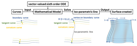
Figure 1.
Overview of the proposed approach.
The contributions of the proposed method include: (1) Compared to the existing patch modeling technique, the proposed technique achieves up to curvature continuities naturally, no manual operations are required to stitch adjacent patches together and deal with the continuity problem between them. (2) Compared with polygon surface and other modeling technique, the data size of character’s 3D model can be sharply compressed and reduced by the proposed method for accelerating network transmission. (3) The global shape of a surface patch can be manipulated easily and efficiently through simply changing one of the first and second partial derivatives at boundary curves and shape control parameters. (4) Since the curves used to define a surface are controlled by differential equations which characterize natural physical process, the proposed technique is one physics-based surface creation method. (5) Compared with other ODE-based surface creation methods, our proposed technique is simpler and more efficient due to its analytical nature.
2. Related Work
Polygon modeling and skin surface creation [1] have been widely applied in commercial available graphics package. This modeling approach can produce detailed or branched models, assign UV texture coordinates, and create hard edges more readily than NURBS modeling. However, polygons are incapable of accurately representing curved surfaces. Therefore, a large number of polygons must be used to approximate curved surfaces in a visually appealing manner. The typical patch modeling approach is NURBS modeling [2,3]. With NURBS modeling, smooth curved objects can be created and edited with few control points. One obvious disadvantage for NURBS modeling is that a lot of manual operations are required to stitch adjacent patches together and deal with the continuity problem between different patches. Subdivision modeling [4,5,6,7] starts the modeling with a coarse polygonal model, subdivides its polygonal faces into smaller faces through approximating or interpolating schemes, and generates a denser polygon mesh of the model. Subdivision makes the modeling of complex geometry more easily and rendering more efficiently. Some disadvantages of subdivision modeling are difficult to specify precision and lack of underlying parametrization. In contrast to the approaches based on trimmed surfaces and control polyhedra, in curved network-based design feature, curves can be directly created and edited in 3D. The method introduced by [8] focuses on special design techniques to adjust the interior of transfinite patches when further shape control is needed.
Physics-based modeling considers the underlying physics of surface deformation. It has the capacity to create more realistic appearances. Various physics-based modeling approaches are reviewed by [9]. These approaches include finite element method, finite difference method [10], finite volume method, mass-spring systems, mesh-free methods, coupled particle systems, and reduced deformable models using modal analysis.
ODEs have been widely applied in scientific computing and engineering analyses to describe the underlying physics. For example, fourth-order ODEs have been used to describe the lateral bending deformations of elastic beams. Introducing ODEs into geometric processing can create physically realistic appearances and deformations of 3D models. ODE-based sweeping surfaces [11], ODE-based surface deformations [12,13], and ODE-based surface blending [14] have also been developed previously. Compared with the conventional surface modeling methods, the ODE-based methods provide the user with a higher level control of the generated surfaces using the parameters and the boundary conditions of the ODE instead of hundreds of control points. Therefore, they can be easily implemented as an easy to use interactive modeling package. However, before that can be realized, one serious hurdle to be overcome, which is to solve the corresponding ODE efficiently. Currently, it is done either ad hoc or only for simple problems. For complicated problems, expensive numerical methods are still the only available choice, such as the finite element method [15,16], finite difference method [10,17], and collocation point method [18]. In order to improve the computational efficiency, the Fourier series method was proposed [19,20]. Although researchers studied ODE-based surface creation and deformations, modeling of curves and surfaces with up to curvature continuities using analytical solutions to ordinary differential equations has not been investigated yet.
3. Mathematical Model
Any 3D parametric surfaces always can be described by the vector-valued mathematical equation , where u and v are two parametric variables usually defined in the region: and , X is a vector-valued position function which has three components x, y, and z, and also has three components , , and . When the parametric variable v takes the constant , the surface at the position becomes a parametric curve , where the vector-valued function has three components , , and . Therefore, the surface can be regarded as the set of the parametric curves , , , which are obtained by changing from 0 to 1 continuously. Based on this consideration, the modelling of 3D parametric surfaces can be transformed into that of a set of parametric curves.
In order to achieve the C2 continuity between two adjacent surface patches, the two surface patches should share the same position function, and first and second partial derivatives with respect to the parametric variable u at their joint should interface. That is to say, a C2 continuous surface patch in the parametric direction u should exactly satisfy the boundary constraints at and which consist of position functions, and the first and second partial derivatives determined by the adjacent surface patches at the positions. If the position functions, and the first and second partial derivatives at the positions and are , the boundary constraints which a C2 continuous surface patch should satisfy can be written as
where and are position functions, and are the first partial derivatives, and and are the second partial derivatives at the boundaries.
With the above treatment, the task of surface modeling is to determine the mathematical equation of the set of the parametric curves which meets Equation (1) at their two ends.
A parametric curve can be described by some popular curve functions such as NURBS. However, these curve functions are purely geometric and did not involve any underlying physics. It has been realized that the physics can be introduced into geometric modeling to improve the realism of geometric modeling and many research studies have addressed physics-based geometric modeling and deformations. Ordinary differential equations (ODEs) usually can be used to describe the deformations of curve-like objects such as beams and members. It is known that the accurate solution of second order ODEs has two unknown constants only which are used to satisfy the constraints of two position functions, and that of fourth order ODEs has four unknown constants which can be used to meet the constraints of two position functions and two first partial derivatives at boundaries. In contrast, the solution of sixth order ODEs contains six unknown constants which can be used to satisfy all the position functions, and the first and second partial derivatives given in boundary constraints Equation (1). Therefore, the following vector-valued sixth order ODE is introduced
where , , and are shape control parameters, represents a 3D parametric curve whose components are , , and , and is the virtual sculpting force function whose components are , , and .
The set of parametric curves can be obtained by finding the solution to Equation (2) subjected to boundary constraints Equation (1). The solution consists of two parts: a complementary solution of the associated homogeneous equation of ODE Equation (2) and a particular solution. In this work, interactive surface creation using the complementary solution is investigated. Surface manipulation using the particular solution will be addressed in the following work.
Before investigating the complementary solution to ODE Equation (2), let us first discuss how to generate the boundary constraints Equation (1). Here, two different approaches are proposed.
The first approach is to draw two boundary curves and , as shown in Figure 2a and Figure 3a. Then boundary tangents and boundary curvature are taken to be the same forms as the boundary curves modified by different coefficients, i.e., , , , and where are different coefficients. Some surfaces generated with this approach were depicted in Figure 2 and Figure 3.
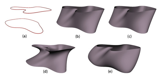
Figure 2.
Closed surface modelling by using two boundary curves.
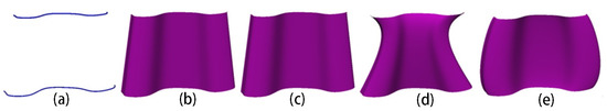
Figure 3.
Open surface modelling by using two boundary curves.
As shown in Figure 4 and Figure 5, the second approach is to create two boundary curves and at and , respectively, and generate the other four control curves at , at , at , where is different from , and at by duplicating the boundary curves and deforming the duplicated curves through some of geometric transformations: translation, scaling, and rotation.
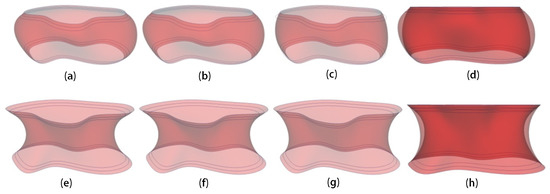
Figure 4.
Closed surface modelling by using two boundary and four control curves.
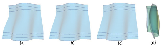
Figure 5.
Open surface modelling by using two boundary and four control curves.
For an arbitrary point on the boundary curve at the position , firstly use the following forward difference formula to calculate the first derivative at the points and , i.e.,
Then the same forward difference formula is used to calculate the second derivative at the point
Similarly, for an arbitrary point on the boundary curve at the position , the following backward difference formula is used to calculate the first derivative at the points and , i.e.,
Next, use the same backward difference formula and the first derivative at the points and to calculate the second derivative at the point
When changes from to , the boundary tangents and boundary curvature in the above equations are continuous functions of the parametric variable v. Therefore, the functions , , , and in Equation (1) can be written as
In Figure 4 and Figure 5, some surfaces which are generated with the second approach are presented.
The surface created by the complementary solution of the associated homogeneous equation of ODE Equation (2) subjected to boundary constraints Equation (1) can be manipulated by the shape control parameters in Equation (2), and the first and second partial derivatives in Equation (1). In order to increase the capacity of surface manipulation, we can further manipulate the created surface through deforming some curves on the surface using the particular solution of ODE Equation (2), which involves a sculpting force represented by the term of the right-hand side of ODE Equation (2). We will address this issue in the following work. The sections below discuss how to achieve the closed form complementary solution of ODE Equation (2) subjected to boundary constraints Equation (1) and use the solution to create various parametric surfaces.
4. Closed Form Complementary Solution
After drawing two boundary curves or 2 boundary curves plus 4 control curves used for the determination of the first and second partial derivatives, the above two approaches can be used to obtain the boundary constraints Equation (1), and create 3D parametric surfaces with the complementary solution of the associated homogeneous equation of ODE Equation (2), i.e.,
subjected to the boundary constraints Equation (1).
The sixth order ODE Equation (2) can be changed into a fourth order ODE by introducing the following vector-valued second order ordinary differential equation
Calculating the second and fourth derivatives of with respect to the parametric variable u and substituting them as well as Equation (9) into Equation (8), the following fourth ODE is reached
The vector-valued ODE Equation (10) can be transformed into an algebra equation by considering
Substituting Equation (11) together with the second and fourth derivatives of with respect to the parametric variable u into Equation (10) and deleting , the following quartic equation is obtained
If is further introduced, the quartic equation Equation (12) is changed into a quadratic equation below
whose roots are
For the sake of conciseness, here only consider the situation of . The other situations can be treated with the same methodology. After substituting Equation (14) into the relation , and introducing two new constants and which are determined by
the following four roots of the quartic equation Equation (12) are obtained
According to the above four roots, the solution to Equation (10) can be written into the following form
where are vector-valued unknown constants. Substituting the above equation into Equation (9) and solving the second order ordinary differential equation, the following solution to the sixth order ordinary differential equation Equation (8) is achieved
where are vector-valued unknown constants. Inserting Equation (18) into the boundary constraints Equation (1), solving for the 6 vector-valued unknown constants , and substituting them back into Equation (18), the following functions which define a 3D parametric surface satisfying the ODE Equation (8) and the boundary constraints Equation (1) exactly is reached:
where
and
5. Continuity between Adjacent Surface Patches
The mathematical equations describing parametric surfaces involve two parametric variables u and v. When parametric surface patches are connected together, they should maintain specified continuities in both u and v parametric directions, shown as Figure 6. In what follows, the continuity in the u parametric direction, and then the continuity in the v parametric direction, will be investigated.
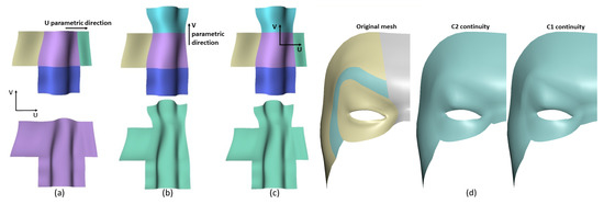
Figure 6.
(a–c) illustrate that our approach can connect surface patches with up to C2 continuities in both u and v parametric directions. (d) shows the comparison between C1 and C2 continuity—our approach can achieve better continuity between patches.
5.1. Continuity in Parametric Direction U
For the continuity of two connected surface patches in the u parametric direction, assuming the two parametric surface patches to be connected together are and , respectively. They are defined by Equation (1) and Equation (8). For the surface patch , the vector-valued function , known vector-valued functions , and shape control parameters , , and in Equations (1) and (2) are replaced by , , and , respectively.
If the two surface patches are required to maintain up to the curvature continuities at the interface where the two surface patches are connected together, the constraints , , and must be satisfied. If the surface patch with the following boundary constraints are created,
continuities of the position, tangent, and curvature between the two surface patches in the u parametric direction are achieved.
5.2. Continuity in Parametric Direction V
For the continuity of two connected surface patches in the v parametric direction, the first and second partial directives of with respect to the parametric variable v are required and can be determined from Equation (19). The first and second partial directives of and the mathematical equations of the surface can be unified as
where indicates the surface of , its first and second partial derivatives with respect to the parametric variable v, respectively, and can be determined from boundary constraints Equation (1).
We still denote the two surface patches to be connected together with and , and use Equations (15), (20)–(22), (26) to determine them and their first and second partial derivatives with respect to the parametric variable v. In the equations, with and without the symbol ∧ on top, denotes for the two adjacent surface patches and and their first and second partial derivatives, respectively.
At the interface where the two surface patches and are to be connected together, the continuity of the position function, and first and second partial derivatives require to be met. According to Equation (26), if and , the constraints are always satisfied.
If setting , have according to Equation (22), from Equation (21), and according to Equation (20). Therefore, two adjacent surface patches achieve up to C2 continuities at their interface if and the position of the boundary curve and its first and second partial derivatives with respect to the parametric variable v for the first surface patch are equal to the ones for the second surface patch at the interface point of the two boundary curves.
The image in Figure 6b is used to visually indicate two surface patches are connected together in the parametric direction v and achieve up to C2 continuities. The shape control parameters for the two surface patches are: , , , , , and and the function of the boundary curves for the two surface patches are and . The experiment in Figure 6c demonstrates that various patches can be smoothly connected together with up to C2 continuities, both in direction u and direction v. In Figure 6d, we decompose the original mesh into 4 parts and recreate the surfaces with C1 and C2 respectively. It indicates the difference between C1 continuity and C2 continuity: (1) C2 continuity can achieve better continuity than C1; (2) and C2 continuity provides the second derivatives as a shape manipulation tool and makes shape manipulation more powerful, as shown in Figure 10.
6. Experiments and Application
Quite a number of experiments are presented to show that the proposed technique achieves up to curvature continuities naturally—no manual operations are required to stitch adjacent patches together and deal with the continuity problem between them. Compared with polygon surfaces, the data size of 3D models can be sharply compressed and reduced by the proposed method for accelerating network transmission. The global shape of a surface patch can be manipulated easily and efficiently through simply changing one of the first and second partial derivatives at boundary curves and shape control parameters.
6.1. Creation of Single Surface
The implemented tool initially uses the first approach to create a closed surface. We draw two boundary curves which were depicted in Figure 2a. The surface created using the Maya loft operation was shown in Figure 2b.
Then, we took the mathematical equation of the first and second partial derivatives to be the same form as the corresponding boundary curves but modified them with the modifying coefficients . When , the surface is generated in Figure 2c, which is the same as that achieved with the Maya loft operation.
If only the first partial derivative is changed and the second partial derivative is kept unchanged, i.e., take , , and , the surface indicated in Figure 2d was produced. If the modifying coefficients were changed into , , and , which means only the second partial derivative was modified, the surface shown in Figure 2e was obtained.
These images indicate that the proposed surface creation method not only can produce surface shapes generated by the Maya loft operation, but also can create different shape changes through manipulating the first and second partial derivatives.
Next, we use the second approach to create a closed surface. Firstly, draw two boundary curves which are the top and bottom ones on the image shown in Figure 4a. Then use the top boundary curve as reference to create another two curves as the control curves of the top boundary curve. Similarly, generate the other two control curves of the bottom boundary curve. Using the Maya loft operation, obtain the surface given in Figure 4a, which interpolates the 2 boundary curves and four control curves. Using Equation (2) to determine the first and second partial derivatives at the top and bottom boundary curves and first taking the shape control parameters to be , and , the surface created with the proposed second approach is given in Figure 4b.
Comparing Figure 4a with Figure 4b, it can be concluded that this approach can also create similar surfaces to those generated by the Maya loft operation. However, this approach has two advantages over the Maya loft operation.
First, this approach can achieve up to C2 continuities between the adjacent patches and there are no manual operations to stitch these adjacent patches together. This is because the two adjacent patches created with this approach share the same first and second partial derivatives.
Second, the shape of the surfaces created with this approach is controllable. This can be demonstrated by comparing Figure 4b and Figure 4c, where the surface in Figure 4c is obtained with the same boundary and control curves as those in Figure 4b but the shape control parameters and are reduced to 0.0001. The shape change between Figure 4b and Figure 4c can be more clearly observed from Figure 4d where the surfaces in Figure 4b,c are shown in the same figure.
If the four control curves in Figure 4a are scaled down, different surfaces are achieved, given in Figure 4e–h where the surface in Figure 4e is from the Maya loft operation, that in Figure 4f is from the proposed second approach with the shape control parameters and , and the one in Figure 4g is from and . Figure 4h is used to compare the surfaces given in Figure 4f,g.
The images in Figure 4 also indicate that the surfaces created with this approach may or may not pass through the four control curves depending on different values of the shape control parameters.
Apart from the applications in creating closed surfaces, the proposed two approaches also apply to open surfaces. We demonstrate this in the following Figure 3 and Figure 5.
In Figure 3, we use two boundary curves and the first approach to create different surface shapes defined by the two boundary curves and different first and second partial derivatives. Figure 3a indicates the two boundary curves, Figure 3b is from the Maya loft operation, Figure 3c–e are from the first approach where Figure 3c is from zeroed first and second partial derivatives, Figure 3d is from the first partial derivative , and zeroed second partial derivative, and Figure 3e is from zeroed first partial derivative and the second partial derivative and . These images also demonstrate that the proposed first approach not only can create those generated by the Maya loft operation, but also those which cannot be obtained from the Maya loft operation.
In Figure 5, we use two boundary curves, four control curves shown in the figure, and the second approach to generate different surface shapes. Figure 5a is generated by the Maya loft operation, Figure 5b is from the second approach and the shape control parameters and , and Figure 5c is from the second approach and the shape control parameters and . The influence of the shape control parameters on surface shapes can be clearly observed from the side view Figure 5d of the surfaces in Figure 5b,c where the surface in yellow is from Figure 5b and the other is from Figure 5c. These images also indicate that the proposed second approach not only creates the surface shapes by the Maya loft operation, but also other surface shapes which cannot be obtained through the Maya loft operation.
6.2. Creation of Complicated Objects
This section introduces how to create complicated objects with the above developed approach. Two approaches will be discussed below.
The first approach is to decompose a surface object into parts. For some complicated parts, they are further decomposed into simple surface patches. The proposed approach is used to create each surface patch which shares the same boundary constraints of position and first and second partial derivatives with the adjacent patch at its four edges.
Taking the dog model in Figure 7a as an example, we first decompose the dog model into parts of head, neck, torso, tail, ears, eyes, front legs, and rear legs. Each of the front legs is further decomposed into three surface patches and each of the rear legs is divided into two surface patches. Then, each surface patch is created and two adjacent patches share the same constraints of the position and the first and second partial derivatives. Besides, the flower model in Figure 7b and plane model in Figure 7c are also created by this approach.
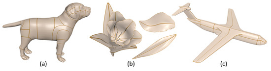
Figure 7.
Creation of surface models by patches.
The second approach is to generate some sketched curves on the model to be created. These sketched curves define some 4-sided and 3-sided patches. For each of 4-sided or 3-sided patches, an ODE surface is created with the constraints of the position and the first and second partial derivative being the same as those of the adjacent surface patches. Here, take the creation of a female face as an example. Some sketched curves in Figure 8a are used to define the plane model, and, accordingly, ODE surface patches are used to build the face model, shown in Figure 8b.
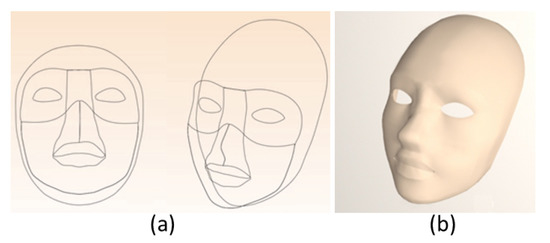
Figure 8.
Creation of surface model by sketch.
From the experiments carried out above, we demonstrate that our approach can compress and reduce the data size of polygon model by just curves, then recreate the surface by our ODE-based method. The recreated model can have the same topology exactly as the original polygon model, as shown in Figure 9, or lower or higher resolution, depending on the parameters chosen by the user, as shown in Figure 10. Table 1 shows the data size comparison between polygon models and our approach. As shown in Figure 7, Figure 8 and Figure 12, in our approach, we only use several boundary curves, and the first and second partial derivatives at the boundary curves to represent and reconstruct the whole original polygon models, so the data size of our approach consists of the vertices’ coordinates of the boundary curves, and the values of first and second derivatives at the boundary curves. Taking the male face model in Figure 12 for instance, the polygon model has 4081 vertices, but the number of vertices on the curves is only 489, in this case, the number of first and second derivatives is 489 as well, so the number of curve variables used by our approach is 1467, and the data size comparison of 36% refers to the curve variables 1467 divided by the original polygon vertices 4081, as shown in the second column of Table 1. This illustrates that the data size of the face model generated by our approach is largely reduced compared with polygon models, being only about one third of original polygon model; the data size of the plane reduced to about one forth; and the data size of the flower model and dog model were reduced to about one fifth of the original polygon models by our approach.
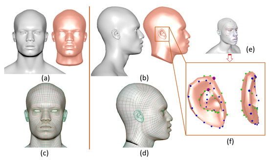
Figure 9.
Global comparison between the face model (red golden) created by the curve network with the proposed method and the original polygon face model (silver).
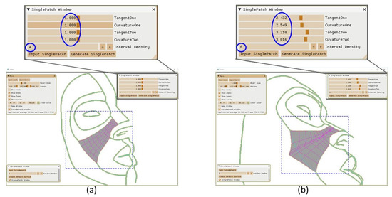
Figure 10.
(a) shows the patch surface generated by default shape control values, (b) shows changing the values of shape control paremeters will generate different surfaces.

Table 1.
The data size comparison between variables of polygon model and our approach.
6.3. One Application of C2 Curve Network for Face Modeling
Face modeling plays a crucial role in both the animation industry and computer graphic academia, in order to obtain high-quality character’s facial shapes for various applications. In this section, one application of the proposed C2 continuous ODE-based surface creation approach is demonstrated. First, one curve network structure is built to represent the 3D facial mesh according to the Facial Action Coding System (FACS) [21], which can be used to obtain diverse face shapes by changing corresponding parameters. Movements of individual facial muscles are encoded by FACS from slightly different instant changes in facial appearance [22]. It is a common standard to systematically categorize the physical expression of emotions, and it has proven useful to psychologists and animators. Using FACS, ref. [23] human coders can manually code nearly any anatomically possible facial expression, deconstructing it into the specific action units (AU) and their temporal segments that produce the expression. As AUs are independent of any interpretation, they can be used for any higher order decision making process including recognition of basic emotions, or pre-programmed commands for an ambient intelligent environment.
As discussed above, the Facial Action Coding System could be used as powerful rules to achieve any anatomically possible facial expression. But how can FACS be implemented and represented by mathematical model to reduce tedious manual work and process more accurately? In order to solve this problem, our work develops one curve network as the mathematical representation of FACS, as shown in Figure 11. Based on the FACS mentioned in the section above, we build the curve network to represent both the neutral human face and approximate diverse facial actions only by several curves. These curves are the basis that can be used accordingly to reconstruct the whole facial model by our C2 continuous ODE surface method.
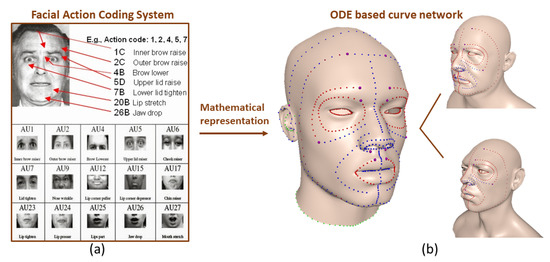
Figure 11.
Mathematical representation of Facial Action Coding System (FACS).
Figure 12 shows the front view and side view of one practical facial curve network structure created by implementing the ODE-based parameterization method, in order to reduce tedious manual work for efficient surface creation. This approach can greatly reduce the data size for facial models compared with polygon models and provide one new and quick way to build different face shapes and expressions by changing the boundary curves and shape control parameters.
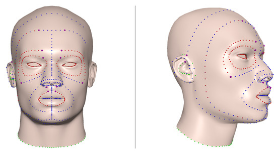
Figure 12.
One face curve network template which can be used to represent and reconstruct different face shapes by our algorithm.
Figure 13 shows the different facial action units reconstructed by the proposed approach which only uses few curves. The first row in Figure 13 shows the polygon models of different Action Units and the curve network (colored curve points) designed for surface representation. The second row shows the red golden area on the right face is reconstructed by curves and the proposed approach, and the remaining area is the original polygon model for comparison. Compare the right side and left side of the models in the third row, the difference between recreated areas (red golden) and original polygon surface can hardly be seen visually. So, the color map is computed for each action unit to show the differences between original and recreated meshes, the Maximum Vertex Errors (MVEs) of AU1, AU2, AU4, and AU9 are 0.011671, 0.013067, 0.020739, and 0.026909, respectively.
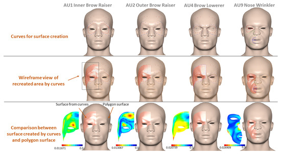
Figure 13.
Reconstruct the surface of different Action Units from few curves by the proposed approach, and compare the realism between reconstructed surfaces and polygon surface.
Figure 9 shows the global comparison between the face model (red golden) created by the curve network with proposed method and the original polygon face model (silver). The front and side views of comparison are shown in (a) and (b). In (c) and (d), the red wireframe is the wireframe of surface created by the curve network, while the green wireframe is from the original polygon surface. From (c) and (d), we can see the surface can be created following the same resolution and edge flow of original model. (e) and (f) show the curve network can also be used to generate detailed areas, such as the ear part, shown in Figure 9f, which uses 4 curves to reconstruct the ear part. The proposed process includes: extracting curve network from one template mesh; generating mesh by curve network and C2 continuous ODE surface method; comparing the reconstructed mesh with original mesh to optimize the shape control parameters.
The obtained results shown in Figure 9 and Figure 13 demonstrate that our method can compress the polygon model into a much smaller data size but still keep the quality of the original model. The data size reduced by the curve network can be seen in Table 1.
The implementation of a GUI for showing the curve network structure and using default parameters to generate initialized surfaces are shown in Figure 14. This implementation of the ODE-based continuous surface creation algorithm is accomplished by C++11 in Visual studio 2017 on a computer with an i7 8650U CPU, 16 GB RAM, and Intel(R) UHD Graphics 620. Figure 14a shows the curve network in the main window and two child windows, the curve network window, and the single patch window. In the curve network window, we can select different numbers of surfaces to create, as shown in Figure 14b,d. Then, Figure 14c,e show the surfaces generated from different input numbers. The above generations depend on the default parameters saved beforehand.
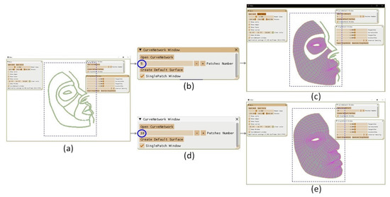
Figure 14.
GUI for showing the curve network structure and use default parameters to generate initialized surfaces.
Instead of using default parameters, the values can be changed in the single patch window to optimize each generated surface shape. The influence of the controller’s value can be seen as Figure 10.
From these experiments, compared to the existing patch modeling technique, the proposed technique achieves up to curvature continuities naturally, and no manual operations are required to stitch adjacent patches together and deal with the continuity problem between them. Compared with polygon surface, the data size of a character’s 3D model can be sharply compressed and reduced by the proposed method for accelerating network transmission. The global shape of a surface patch can be manipulated easily and efficiently through simply changing one of the first and second partial derivatives at boundary curves and shape control parameters.
7. Discussion and Conclusions
In this paper, an efficient ODE-based surface generation technique has been proposed to create C2 continuous surfaces. This technique is based on the mathematical model consisting of a vector-valued sixth order ordinary differential equation and C2 continuous boundary constraints.
The solution to the vector-valued sixth order ordinary differential equation is a three-dimensional curve which is used to define an iso-parametric line of surface models. By making an isoparametric line satisfying the constraints of the position, and the first and second partial derivatives, a surface patch is created. The surface models consisting of such surface patches always maintain C2 continuity between different surface patches.
In order to create surface patches quickly, the analytical solution to the vector-valued sixth order ordinary differential equation subjected to the constraints of position and the first and second partial derivatives is developed. With the obtained analytical solution, the users only generate two boundary curves or two boundary curves plus four control curves, the proposed approach transforms them into the boundary constraints of the position and the first and second derivatives, and creates a surface patch precisely satisfying these constraints.
When building surface models, existing patch modeling techniques require tedious and time-consuming manual operations to stitch two separate patches together to achieve tangential or curvature continuity. The technique proposed in this work solves this problem. All created surface patches are connected together automatically with C2 continuity. Moreover, the technique can largely reduce the data size of polygon model, especially suitable for quick network transmission. Besides, the proposed approach introduces physics to improve the realism of geometric modeling.
Author Contributions
All authors contributed to the paper, and approved the present version to be published. All authors have read and agreed to the published version of the manuscript.
Acknowledgments
This research is supported by Innovate UK (Knowledge Transfer Partnerships Ref: KTP010860) and the EU Horizon 2020 RISE 2017 funded project PDE-GIR (H2020-MSCA-RISE-2017-778035). Shaojun Bian is also supported by China Scholarship Council.
Conflicts of Interest
The authors declare no conflict of interest.
References
- Russo, M. Polygonal Modeling: Basic and Advanced Techniques; Jones & Bartlett Learning: Burlington, MA, USA, 2006. [Google Scholar]
- Piegl, L.; Tiller, W. The NURBS Book; Springer Science & Business Media: Berlin/Heidelberg, Germany, 2012. [Google Scholar]
- Farin, G. Curves and Surfaces for Computer-Aided Geometric Design: A Practical Guide; Elsevier: Amsterdam, The Netherlands, 2014. [Google Scholar]
- Stam, J. Exact evaluation of Catmull-Clark subdivision surfaces at arbitrary parameter values. In Proceedings of the 25th Annual Conference on Computer Graphics and Interactive Techniques, Orlando, FL, USA, 19–24 July 1998; ACM: New York, NY, USA, 1998; pp. 395–404. [Google Scholar]
- DeRose, T.; Kass, M.; Truong, T. Subdivision surfaces in character animation. In Proceedings of the 25th Annual Conference on Computer Graphics and Interactive Techniques, Orlando, FL, USA, 19–24 July 1998; ACM: New York, NY, USA, 1998; pp. 85–94. [Google Scholar]
- Warren, J.; Weimer, H. Subdivision Methods for Geometric Design: A Constructive Approach; Morgan Kaufmann: Burlington, MA, USA, 2001. [Google Scholar]
- Cashman, T.J.; Augsdörfer, U.H.; Dodgson, N.A.; Sabin, M.A. NURBS with extraordinary points: high-degree, non-uniform, rational subdivision schemes. In ACM Transactions on Graphics (TOG); ACM: New York, NY, USA, 2009; Volume 28, p. 46. [Google Scholar]
- Várady, T.; Salvi, P.; Rockwood, A. Transfinite surface interpolation with interior control. Graph. Model. 2012, 74, 311–320. [Google Scholar] [CrossRef]
- Nealen, A.; Müller, M.; Keiser, R.; Boxerman, E.; Carlson, M. Physically Based Deformable Models in Computer Graphics. Computer Graphics Forum; Wiley: Hoboken, NJ, USA, 2006; Volume 25, pp. 809–836. [Google Scholar]
- Chaudhry, E.; Bian, S.; Ugail, H.; Jin, X.; You, L.; Zhang, J.J. Dynamic skin deformation using finite difference solutions for character animation. Comput. Graph. 2015, 46, 294–305. [Google Scholar] [CrossRef]
- You, L.; Yang, X.; Pachulski, M.; Zhang, J.J. Boundary Constrained Swept Surfaces for Modelling and Animation. Computer Graphics Forum; Wiley: Hoboken, NJ, USA, 2007; Volume 26, pp. 313–322. [Google Scholar]
- You, L.; Yang, X.; You, X.Y.; Jin, X.; Zhang, J.J. Shape manipulation using physically based wire deformations. Comput. Animat. Virtual Worlds 2010, 21, 297–309. [Google Scholar] [CrossRef]
- Chaudhry, E.; You, L.; Jin, X.; Yang, X.; Zhang, J.J. Shape modeling for animated characters using ordinary differential equations. Comput. Graph. 2013, 37, 638–644. [Google Scholar] [CrossRef]
- You, L.; Ugail, H.; Tang, B.; Jin, X.; You, X.Y.; Zhang, J.J. Blending using ODE swept surfaces with shape control and C1 continuity. Vis. Comput. 2014, 30, 625–636. [Google Scholar] [CrossRef]
- Li, Z.C. Boundary penalty finite element methods for blending surfaces, I basic theory. J. Comput. Math. 1998, 110, 457–480. [Google Scholar]
- Li, Z.C.; Chang, C.S. Boundary penalty finite element methods for blending surfaces, III. Superconvergence and stability and examples. J. Comput. Appl. Math. 1999, 110, 241–270. [Google Scholar] [CrossRef]
- Cheng, S.; Bloor, M.I.; Saia, A.; Wilson, M.J. Blending between quadric surfaces using partial differential equations. Adv. Des. Autom. 1990, 1, 257–263. [Google Scholar]
- Bloor, M.I.; Wilson, M.J. Representing PDE surfaces in terms of B-splines. Comput. Aided Des. 1990, 22, 324–331. [Google Scholar] [CrossRef]
- Bloor, I.M.; Wilson, M.J. Spectral approximations to PDE surfaces. Comput. Aided Des. 1996, 28, 145–152. [Google Scholar] [CrossRef]
- Bian, S.; Deng, Z.; Chaudhry, E.; You, L.; Yang, X.; Guo, L.; Ugail, H.; Jin, X.; Xiao, Z.; Zhang, J.J. Efficient and realistic character animation through analytical physics-based skin deformation. Graph. Models 2019, 104, 101035. [Google Scholar] [CrossRef]
- Paul, E.; Wallace, F.V.; Joseph, H.C. Facial Action Coding System. The Manual on CD ROM; A Human Face: Salt Lake City, UT, USA, 2002. [Google Scholar]
- Hamm, J.; Kohler, C.G.; Gur, R.C.; Verma, R. Automated facial action coding system for dynamic analysis of facial expressions in neuropsychiatric disorders. J. Neurosci. Methods 2011, 200, 237–256. [Google Scholar] [CrossRef] [PubMed]
- Freitas-Magalhães, A. The Face of Lies; Leya: Amadora, Portugal, 2013. [Google Scholar]
© 2019 by the authors. Licensee MDPI, Basel, Switzerland. This article is an open access article distributed under the terms and conditions of the Creative Commons Attribution (CC BY) license (http://creativecommons.org/licenses/by/4.0/).