The Generalized Distance Spectrum of the Join of Graphs

Abstract

Let G be a simple connected graph. In this paper, we study the spectral properties of the generalized distance matrix of graphs, the convex combination of the symmetric distance matrix $D\left(G\right)$ and diagonal matrix of the vertex transmissions $Tr\left(G\right)$. We determine the spectrum of the join of two graphs and of the join of a regular graph with another graph, which is the union of two different regular graphs. Moreover, thanks to the symmetry of the matrices involved, we study the generalized distance spectrum of the graphs obtained by generalization of the join graph operation through their eigenvalues of adjacency matrices and some auxiliary matrices.

1. Introduction

Complicated graph structures can often be built from relatively simple graphs via graph-theoretic binary operations such as products. Graph spectrum provides a unique way of characterizing graph structures, sometimes even identifying the entire graph classes. Moreover, using simple graph operations, the spectra of complicated graphs may be constructed from those of small and simple graphs. The interplay between graph spectra (including adjacency, Laplacian, etc.) and various binary graph operations such as corona, edge corona, and disjoint union has been extensively studied in the literature; see e.g., [1,2,3,4,5,6].

In this paper, we consider simple connected graphs [7]. A graph G is represented by $G=\left(V\right(G),E(G\left)\right)$, in which the set $V\left(G\right)=\{v_1,v_2,\dots ,v_n\}$ represents its vertex set and $E\left(G\right)$ is the edge set connecting pairs of distinct vertices. The number $n=\left|V\right(G\left)\right|$ is referred to as the order of G and $\left|E\right(G\left)\right|$ is the size of it. A vertix adjacent to a vertex $v\in V\left(G\right)$ is called the neighborhood of v and is presented by $N\left(v\right)$. The degree of a vertex v is the cardinality of its neighborhood and denoted by $d_G\left(v\right)$ or simply $d_v$. A regular graph has the same degree for all vertices. The distance $d_{uv}$ is the length of a shortest path between two vertices u and v. The maximum distance between two vertices is called the diameter of a graph. The matrix $D\left(G\right)={\left(d_{uv}\right)}_{u,v\in V\left(G\right)}$ is called the distance matrix of G. As usual, $\overline{G}$ is the complement of the graph G. Moreover, the complete graph $K_n$, the complete bipartite graph $K_{s,t}$, the path $P_n$, the cycle $C_n$, and the wheel graph $W_n$ are defined in the conventional way. The sum of the distances from a vertex v to all other vertices, $T{r}_G\left(v\right)={\displaystyle \sum _{u\in V\left(G\right)}}{d}_{uv}$, is called the transmission degree of v. A k-transmission regular graph admits $T{r}_G\left(v\right)=k$ for any vertex v. Let $T{r}_i=T{r}_G\left(v_i\right)$. Then the sequence $\{T{r}_1,T{r}_2,\dots ,T{r}_n\}$ is said to be the transmission degree sequence. The quantity ${\displaystyle T_i:=\sum _{j=1}^n{d}_{ij}T{r}_j}$ is referred to as the second transmission degree of $v_i$.

The diagonal matrix $Tr\left(G\right):=diag(T{r}_1,T{r}_2,\dots ,T{r}_n)$ characterizes the vertex transmissions of G. For a connected graph, M. Aouchiche and P. Hansen [8,9] studied the Laplacian and the signless Laplacian for its distance matrix. The distance Laplacian matrix $D^L\left(G\right)=Tr\left(G\right)-D\left(G\right)$ and the distance signless Laplacian matrix $D^Q\left(G\right)=Tr\left(G\right)+D\left(G\right)$ have attracted great recent research attention due to their usefulness in spectrum theory. Recently, Cui et al. [10] investigated a convex combination of $Tr\left(G\right)$ and $D\left(G\right)$ in the form of $D_{\alpha }\left(G\right)=\alpha Tr\left(G\right)+(1-\alpha )D\left(G\right),$ $0\le \alpha \le 1,$ which is called the generalized distance matrix. Through the study of generalized distance matrix, not only new results can be derived but existing results can be looked into in a new unified point of view.

Let I be the identity matrix of order n. The characteristic polynomial of $D_{\alpha }\left(G\right)$ can be written as $\psi (G:\partial )=\det (\partial I-D_{\alpha }\left(G\right))$. The generalized distance eigenvalues of G are the zeros of $\psi (G:\partial )$. Noting that $D_{\alpha }\left(G\right)$ is real and symmetric, we arrange the eigenvalues as ${\partial }_1\ge {\partial }_2\ge \cdots \ge {\partial }_n$. We call ${\partial }_1$ the generalized distance spectral radius of G. The generalized distance spectrum and energy have been recently scoped in [11,12].

The rest of the paper is organized as follows. In Section 2, we study the generalized distance spectrum of join of regular graphs. We will show that the generalized distance spectrum of join of two regular graphs can be obtained from their adjacency spectrum. Again using adjacency eigenvalues, we determine the generalized distance spectrum of join of a regular graph with the union of two different regular graphs. In Section 3, we use the adjacency matrix eigenvalues and auxiliary matrices to characterize the generalized distance spectrum of the joined union of regular graphs.

2. On the Generalized Distance Spectrum of Join of Graphs

In this section, we study the generalized distance spectrum of join of regular graphs. We will establish new relationship between generalized distance spectrum and adjacency spectrum. As applications, we obtain the generalized distance spectrum of some special graph classes including complete bipartite graph, complete split graph, wheel graph and some derived graphs from a complete graph.

Consider two disjoint vertex sets $V_1$ and $V_2$ with $|V_1|=n_1$ and $|V_2|=n_2$. For two graphs $G_1=(V_1,E_1)$ and $G_2=(V_2,E_2)$, the union is $G_1\cup G_2=(V_1\cup V_2,E_1\cup E_2)$. The join of them is denoted by $G_1\nabla G_2$ consisting of $G_1\cup G_2$ and all edges joining each vertex in $V_1$ and each vertex in $V_2.$ In other words, the join of them can be obtained by connecting each vertex of $G_1$ to all vertices of $G_2.$

The following gives the generalized distance spectrum of join of two regular graphs in terms of their eigenvalues of adjacency matrices.

Theorem 1.

Let $G_i$ be an $r_i$-regular graph of order $n_i$, for $i=1,2.$ Let $r_1={\lambda }_1,{\lambda }_2,\cdots ,{\lambda }_{n_1}$ and $r_2={\mu }_1,{\mu }_2,\cdots ,{\mu }_{n_2}$ are the adjacency eigenvalues of $G_1$ and $G_2$, respectively. The characteristic polynomial of the generalized distance matrix of $G_1\nabla G_2$ is given by

$$\begin{array}{c}\psi (G_1\nabla G_2:x)=[x^2-({\gamma }_1+{\gamma }_2-(1-\alpha )(n_1+n_2))x+{\gamma }_1{\gamma }_2-{\gamma }_1{n}_1(1-\alpha )-{\gamma }_2{n}_2(1-\alpha )]\\ \prod _{i=2}^{n_1}\left(x-\alpha {\gamma }_1+(1-\alpha )({\lambda }_i+2)\right)\prod _{j=2}^{n_2}\left(x-\alpha {\gamma }_2+(1-\alpha )({\mu }_j+2)\right),\end{array}$$

where ${\gamma }_1=2n_1+n_2-r_1-2$ and ${\gamma }_2=2n_2+n_1-r_2-2$.

Proof. 

For $i=1,2$, let $G_i$ be an $r_i$-regular graph of order $n_i$. Let $G=G_1\nabla G_2$ be the join of the graphs $G_1$ and $G_2$. It is clear that G is graph of diameter 2. Let $V\left(G_i\right)=\{v_{i1},v_{i2},\cdots ,v_{i{n}_i}\}$ be the vertex set of the graph $G_i$, then the vertex set of G is $V\left(G\right)=V\left(G_1\right)\cup V\left(G_2\right)$. For all $v\in V\left(G_1\right)$, we have $Tr\left(v\right)=2n_1+n_2-r_1-2$ and for all $u\in V\left(G_2\right)$, we have $Tr\left(u\right)=2n_2+n_1-r_2-2$. Let us label the vertices of G, so that the first $n_1$ vertices are from $G_1$. Under this labelling, it can be seen that the generalized distance matrix of G can be written as

$$\begin{array}{c}\hfill D_{\alpha }\left(G\right)=\left(\begin{array}{cc}\alpha {\gamma }_1{I}_{n_1}+(1-\alpha )(A_1+2{\overline{A}}_1)& (1-\alpha )J_{n_1\times n_2}\\ (1-\alpha )J_{n_2\times n_1}& \alpha {\gamma }_2{I}_{n_2}+(1-\alpha )(A_2+2{\overline{A}}_2)\end{array}\right),\end{array}$$

where ${\gamma }_1=2n_1+n_2-r_1-2$, ${\gamma }_2=2n_2+n_1-r_2-2$, $J_{n_1\times n_2}$ is an all one matrix, $I_{n_i}$ is the identity matrix of order $n_i$, $A_i$ is the adjacency matrix of $G_i$ and ${\overline{A}}_i$ is the adjacency matrix of the complement ${\overline{G}}_i$, for $i=1,2.$

Since $G_i$ is an $r_i$-regular graph, it follows that $e_{n_i}={(1,1,\cdots ,1)}^T$, the all ones vector of order $n_i$, is an eigenvector corresponding to the eigenvalue $r_i$ of $A_i$ and corresponding to the eigenvalue $n_i-1-r_i$ of ${\overline{A}}_i$. Let x be a vector orthogonal to $e_{n_1}$, satisfying $A_{1}x=\lambda x$, then ${\overline{A}}_{1}x=(-\lambda -1)x$. Taking $X=\left(\begin{array}{c}x\\ 0\end{array}\right)$ and using $J_{n_1\times n_2}x=0$, we have $D_{\alpha }\left(G\right)X=[\alpha {\gamma }_1-(1-\alpha )(\lambda +2)]X$. This shows that $\alpha {\gamma }_1-(1-\alpha )(\lambda +2)$ is an eigenvalue of $D_{\alpha }\left(G\right)$ corresponding to the eigenvalue $\lambda$ of $A_1$. Let y be a vector orthogonal to $e_{n_2}$, satisfying $A_{2}y=\mu y$, then ${\overline{A}}_{2}y=(-\mu -1)y$. Taking $Y=\left(\begin{array}{c}0\\ y\end{array}\right)$ and using $J_{n_2\times n_1}y=0$, we have $D_{\alpha }\left(G\right)Y=[\alpha {\gamma }_2-(1-\alpha )(\mu +2)]Y$. This shows that $\alpha {\gamma }_2-(1-\alpha )(\mu +2)$ is an eigenvalue of $D_{\alpha }\left(G\right)$ corresponding to the eigenvalue $\mu$ of $A_2$. The equitable quotient matrix of $D_{\alpha }\left(G\right)$ is

$$\begin{array}{c}\hfill M=\left(\begin{array}{cc}\alpha n_2+2n_1-r_1-2& (1-\alpha )n_2\\ (1-\alpha )n_1& \alpha n_1+2n_2-r_2-2\end{array}\right).\end{array}$$

Since the characteristic polynomial of M is $x^2-({\gamma }_1+{\gamma }_2-(1-\alpha )(n_1+n_2))x+{\gamma }_1{\gamma }_2-{\gamma }_1{n}_1(1-\alpha )-{\gamma }_2{n}_2(1-\alpha )$ and any eigenvalue of M is an eigenvalue of $D_{\alpha }\left(G\right)$ [13], the result follows. □

Let $K_{r,s}$ be the complete bipartite graph. It is well-known that $K_{r,s}={\overline{K}}_r\nabla {\overline{K}}_s$. We have the following observation from Theorem 1, which gives the generalized distance spectrum of $K_{r,s}$.

Corollary 1.

The generalized distance eigenvalues of $K_{r,s}$ consists of the eigenvalue $\alpha (2r+s)-2$ with multiplicity $r-1$, the eigenvalue $\alpha (2s+r)-2$ with multiplicity $s-1$ and the eigenvalues $x_1,x_2=\frac{\alpha (s+r)+2(s+r)-4\pm \sqrt{(r^2+s^2){(\alpha -2)}^2+2rs({\alpha }^2-2)}}{2}$.

Proof. 

Similarly as in Theorem 1, this can be proved by taking $n_1=r,n_2=s,r_1=r_2=0$ and ${\lambda }_i={\mu }_j=0$, for all $i,j$. □

Let $W_{n+1}$ be the wheel graph of order $n+1$. It is well known that $W_{n+1}=C_n\nabla K_1$. Using the fact that the adjacency spectrum of $C_n$ is $\{2cos\left(\frac{2\pi (j-1)}{n}\right):j=1,2,\cdots ,n\}$, we have the following observation from Theorem 1, which gives the generalized distance spectrum of $W_{n+1}$.

Corollary 2.

The generalized distance eigenvalues of the wheel graph $W_{n+1}$ consists of the eigenvalues $\alpha (2n-3)-(1-\alpha )(2+2cos\left(\frac{2\pi (i-1)}{2}\right)),i=2,3,\cdots ,n$ and also the eigenvalues $x_1,x_2=\frac{(\alpha +2)n+\alpha -4\pm \sqrt{{[(\alpha +2)n+\alpha -4]}^2-8\alpha n(n-1)+4n}}{2}$.

Proof. 

Proof follows from Theorem 1, by taking $n_1=n,n_2=1,r_1=2,r_2=0$ and ${\lambda }_i=2cos\left(\frac{2\pi (i-1)}{n}\right),$ for $i=2,3,\cdots ,n$. □

The graph $C{S}_{t,n-t}$ of order n is called complete split graph. It is constructed by linking each vertex of a clique of t vertices to each vertex of an independent set of $n-t$ vertices. It is clear that $C{S}_{t,n-t}=K_t\nabla {\overline{K}}_{n-t}$. Using the fact that the adjacency spectrum of $K_t$ is $\{t-1,-1^{[t-1]}\}$, we have the following observation from Theorem 1, which gives the generalized distance spectrum of $C{S}_{t,n-t}$.

Corollary 3.

The generalized distance eigenvalues of $C{S}_{t,n-t}$ consists of the eigenvalues $\alpha n-1$ with multiplicity $t-1$, the eigenvalue $\alpha (2n-t)-2$ with multiplicity $n-t-1$ and the eigenvalues$x_1,x_2=\frac{2n-t+\alpha n-3\pm \sqrt{\theta }}{2}$, $\theta =(5-4\alpha )t^2+(6\alpha n-8n-4\alpha +6)t+n^2{(\alpha -2)}^2+2n\alpha -4n+1$.

Proof. 

Similarly as in Theorem 1, this can be shown by taking $n_1=t,n_2=n-t,r_1=t-1,r_2=0$, ${\lambda }_i=-1,$ for $i=2,3,\cdots ,t$ and ${\mu }_j=0$, for $j=2,3,\cdots ,n-t$. □

In the next result, we work out the relationship between the generalized distance spectrum of the join of regular graphs and their adjacency spectra.

Theorem 2.

For $i=0,1,2,$ let $G_i$ be $r_i$-regular with order $n_i$. Let $A\left(G_i\right)$ be their adjacency matrices and the adjacency eigenvalues are ${\lambda }_{i,1}=r_i\ge {\lambda }_{i,2}\ge \dots \ge {\lambda }_{i,n_i}$. We have that the generalized distance spectrum of $G_0\nabla (G_1\cup G_2)$ is eigenvalues $\alpha (m+n_0+{\lambda }_{0,j}-r_0)-{\lambda }_{0,j}-2$ for $j=2,\dots ,n_0,$ and $\alpha (2m-n_0+{\lambda }_{i,j}-r_i)-{\lambda }_{i,j}-2,$ for $i=1,2$ and $j=2,3,\dots ,n_i,$ where $m={\sum }_{i=0}^2{n}_i,$ and three extra eigenvalues defined by the eigenvalues of the following matrix

$$\left(\begin{array}{ccc}{\mathsf{\Theta }}_0& (1-\alpha )n_1& (1-\alpha )n_2\\ (1-\alpha )n_0& {\mathsf{\Theta }}_1& 2(1-\alpha )n_2\\ (1-\alpha )n_0& 2(1-\alpha )n_1& {\mathsf{\Theta }}_2\end{array}\right),$$

(1)

where ${\mathsf{\Theta }}_0=\alpha (m-n_0)+2n_0-r_0-2,$ and ${\mathsf{\Theta }}_i=\alpha (2m-n_0-2n_i)+2n_i-r_i-2,$ $i=1,2.$

Proof. 

Given $i=0,1,2$. Assume $G_i$ is $r_i$-regular and has $n_i$ vertices. Let $G=G_0\nabla (G_1\cup G_2)$ be the join of the graphs $G_0$ and $G_1\cup G_2$. Obviously, G has diameter 2. Let $V\left(G_i\right)=\{v_{i1},v_{i2},\cdots ,v_{i{n}_i}\}$ be the vertex set of the graph $G_i$, then the vertex set of G is $V\left(G\right)=V\left(G_0\right)\cup V\left(G_1\right)\cup V\left(G_2\right)$. For all $v\in V\left(G_0\right)$, we have $Tr\left(v\right)=m+n_0-r_0-2$, for all $u\in V\left(G_1\right)$, we have $Tr\left(v\right)=2m-n_0-r_1-2$ and for all $w\in V\left(G_2\right)$, we have $Tr\left(w\right)=2m-n_0-r_2-2$. Let us label the vertices of G, so that the first $n_0$ vertices are from $G_0$, the next $n_1$ vertices are from $G_1$ and the next $n_2$ vertices are from $G_2$. Under this labelling, the generalized distance matrix of G has the form

$$D_{\alpha }\left(G\right)=\left(\begin{array}{ccc}{S}_0& (1-\alpha )J_{n_0\times n_1}& (1-\alpha )J_{n_0\times n_2}\\ (1-\alpha )J_{n_1\times n_0}& S_1& 2(1-\alpha )J_{n_1\times n_2}\\ (1-\alpha )J_{n_2\times n_0}& 2(1-\alpha )J_{n_2\times n_1}& S_2\end{array}\right),$$

where $S_0=\alpha \left((m+n_0-r_0)I_{n_0}+A\left(G_0\right)-2J_{n_0}\right)+2(J_{n_0}-I_{n_0})-A\left(G_0\right),$ and $S_i=\alpha \left((2m-n_0-r_i)I_{n_i}+A\left(G_i\right)-2J_{n_i}\right)+2(J_{n_i}-I_{n_i})-A\left(G_i\right),$ for $i=1,2.$

For a regular graph $G_i$, the all ones vector $e_{n_i}={(1,1,\cdots ,1)}^T$ of order $n_i$ is an eigenvector corresponding to the eigenvalue $r_i$. Other eigenvectors are orthogonal to $e_{n_i}$. Therefore, the all ones vector $e_{n_0}={(1,1,\cdots ,1)}^T$ of order $n_0$ is an eigenvector corresponding to the eigenvalue $r_0$. Other eigenvectors are orthogonal to $e_{n_0}.$ Suppose that $\lambda$ be an eigenvalue of adjacency matrix of $G_0$ and its eigenvector is x satisfying $e_{n_0}^{T}x=0,$ then ${\left(x^T{0}_{1\times n_1}{0}_{1\times n_2}\right)}^T$ is an eigenvector of $D_{\alpha }\left(G\right)$ with the eigenvalue $\alpha (m+n_0+\lambda -r_0)-\lambda -2.$ Let $\mu ,\xi$ be any eigenvalues of the adjacency matrix of $G_1$ and $G_2$ with associated eigenvector y and z satisfying $e_{n_1}^{T}y=0,e_{n_2}^{T}z=0$, respectively. In a similar way, it can be seen that the vectors ${\left(0_{1\times n_0}{y}^T{0}_{1\times n_2}\right)}^T$ and ${\left(0_{1\times n_0}{0}_{1\times n_1}{z}^T\right)}^T$ are eigenvectors of $D_{\alpha }\left(G\right)$ with corresponding eigenvalues $\alpha (2m-n_0+\mu -r_1)-\mu -2$ and $\alpha (2m-n_0+\xi -r_2)-\xi -2,$ respectively.

Hence, we obtained eigenvectors ${\left(x^T{0}_{1\times n_1}{0}_{1\times n_2}\right)}^T,$ ${\left(0_{1\times n_0}{y}^T{0}_{1\times n_2}\right)}^T$ and $(0_{1\times n_0}{0}_{1\times n_1}$ $z^T{)}^T$. They are $m-3$ eigenvectors. It is easy to see that they are orthogonal to ${\left(e_{n_0}^T{0}_{1\times n_1}{0}_{1\times n_2}\right)}^T,$ ${\left(0_{1\times n_0}{e}_{n_1}^T{0}_{1\times n_2}\right)}^T$ and ${\left(0_{1\times n_0}{0}_{1\times n_1}{e}_{n_2}^T\right)}^T.$ All other three eigenvectors of $D_{\alpha }\left(G\right)$ can be represented by ${\left(\beta e_{n_0}^T\gamma e_{n_1}^T\theta e_{n_2}^T\right)}^T$ for some $(\beta ,\gamma ,\theta )\ne (0,0,0).$

Suppose that $\nu$ is an eigenvalue of the matrix $D_{\alpha }\left(G\right)$ with associated eigenvector $X={(\beta e_{n_0}^T,\gamma e_{n_1}^T,\theta e_{n_2}^T)}^T$. Recall that $D_{\alpha }\left(G\right)X=\nu X,$ and $A\left(G_i\right)e_{n_i}=r_i{e}_{n_i}$ ($i=0,1,2$). We obtain:

$$\begin{array}{c}(\alpha (m-n_0)+2n_0-r_0-2)\beta +(1-\alpha )n_1\gamma +(1-\alpha )n_2\theta =\nu \beta ,\hfill \\ (1-\alpha )n_0\beta +(\alpha (2m-n_0-2n_1)+2n_1-r_1-2)\gamma +2(1-\alpha )n_2\theta =\nu \gamma ,\hfill \\ (1-\alpha )n_0\beta +2(1-\alpha )n_1\gamma +(\alpha (2m-n_0-2n_2)+2n_2-r_2-2)\theta =\nu \theta .\hfill \end{array}$$

These equations admit a nontrivial solution only if (1) has an eigenvalue $\nu$. Moreover, any nontrivial solution of the equations is an eigenvector of $D_{\alpha }\left(G\right)$ associated to $\nu .$ As the remaining three eigenvectors of $D_{\alpha }\left(G\right)$ are formed like this, it is obvious that any eigenvalue of (1) is also an eigenvalue of $D_{\alpha }\left(G\right)$. □

Consider the graph $G(n_0,n_1,n_2)=K_{n_0}\nabla (K_{n_1}\cup K_{n_2})$. We have the following observation from Theorem 2, which gives the generalized distance spectrum of $G(n_0,n_1,n_2)$.

Corollary 4.

The generalized distance eigenvalues of $G(n_0,n_1,n_2)$ consists of eigenvalue $\alpha m-1$, with multiplicity $n_0-1$, the eigenvalue $\alpha (2m-n_0-n_1)-1,$ with multiplicity $n_1-1$, the eigenvalue $\alpha (2m-n_0-n_2)-1,$ with multiplicity $n_2-1$ and three more eigenvalues which are the eigenvalues of the matrix

$$\left(\begin{array}{ccc}\alpha (m-n_0)+n_0-1& (1-\alpha )n_1& (1-\alpha )n_2\\ (1-\alpha )n_0& \alpha (2m-n_0-2n_1)+n_1-1& 2(1-\alpha )n_2\\ (1-\alpha )n_0& 2(1-\alpha )n_1& \alpha (2m-n_0-2n_2)+n_2-1\end{array}\right),$$

where $m={\sum }_{i=0}^2{n}_i$.

Proof. 

Proof follows from Theorem 2, by taking $r_0=n_0-1,r_1=n_1-1,r_2=n_2-1,{\lambda }_{i,j}=-1$, for all $i=0,1,2$ and $j=2,3,\cdots ,n_i$. □

Suppose we have a complete graph $K_n$ of order n. The graph $K_n-e$ is obtained by removing an edge e from $K_n$. Taking $n_0=n-2,n_1=n_2=1$ and $m=n$, in Corollary 4, we obtain the generalized distance spectrum of the graph $K_n-e$ given by $\{\alpha n-1^{[n-3]},x_1,x_2,x_3\}$, where $x_1,x_2$ and $x_3$ are the roots of the equation $f\left(x\right)=x^3-[2\alpha (n+1)+n-3]x^2+[(n^2+2n){\alpha }^2+2n(n-1)\alpha -2n]x-[(n^3+n^2+4){\alpha }^2-2\alpha (n^2+4)+4]=0$.

3. The Generalized Distance Spectrum of the Joined Union

In this section, we describe the relationship between generalized distance spectrum and the adjacency spectrum of the joined union of regular graphs.

The spectrum of a graph may determine the class of graphs that share the same properties. There have been some different names for the binary graph operation to be introduced below. We will call it joined union following [4,6]. This operation is also called generalized composition [14] or H-join [3]. Let $G=(V,E)$ have order n and $G_i=(V_i,E_i)$ have order $m_i,$ for $i=1,\dots ,n$. The joined union $G[G_1,\dots ,G_n]$ is the graph $H=(W,F)$ satisfying:

$$\begin{array}{ccc}\hfill W& =& \bigcup _{i=1}^n{V}_i\hfill \\ \hfill \mathrm{and}F& =& \bigcup _{i=1}^n{E}_i\cup \bigcup _{\{v_i,v_j\}\in E}{V}_i\times V_j.\hfill \end{array}$$

Clearly, the joined union graph can be constructed by taking the union of $G_1,\dots ,G_n$ and linking any pair of vertices between $G_i$ and $G_j$ if $v_i$ and $v_j$ are neighbors in $G.$ By this definition, the usual join of $G_1$ and $G_2$ can be viewed as $K_2[G_1,G_2]$, which is a special joined union graph.

Theorem 3.

Suppose G is a graph with diameter at most 2 over $V\left(G\right)=\{v_1,\dots ,v_n\}$. Denote by $G_i$ an $r_i$-regular graph of order $m_i$ and adjacency eigenvalues ${\lambda }_{i1}=r_i\ge {\lambda }_{i2}\ge \dots \ge {\lambda }_{i{m}_i},$ where $i=1,2,\dots ,n.$ The generalized distance spectrum of the joined union $G[G_1,\dots ,G_n]$ consists of the eigenvalues $\alpha (2m+{\lambda }_{ik}-m_i^{\prime }-r_i)-{\lambda }_{ik}-2$ for $i=1,\dots ,n$ and $k=2,3,\dots ,m_i$, where ${\displaystyle m=\sum _{i=1}^n{m}_i}$ and ${\displaystyle m_i^{\prime }=\sum _{v_i{v}_j\in E\left(G\right)}{m}_j}$. The remaining n eigenvalues are given by the matrix

$$\left(\begin{array}{cccc}{M}_{1,1}& (1-\alpha )m_2{d}_G(v_1,v_2)& \dots & (1-\alpha )m_n{d}_G(v_1,v_n)\\ (1-\alpha )m_1{d}_G(v_2,v_1)& M_{2,2}& \dots & (1-\alpha )m_n{d}_G(v_2,v_n)\\ ⋮& ⋮& \ddots & ⋮\\ (1-\alpha )m_1{d}_G(v_n,v_1)& (1-\alpha )m_2{d}_G(v_n,v_2)& \dots & M_{n,n}\end{array}\right),$$

(2)

where $M_{i,i}=\alpha (2m-2m_i-m_i^{\prime })+2m_i-r_i-2.$

Proof. 

Let G be a graph over $V\left(G\right)=\{v_1,\dots ,v_n\}$ and let $V\left(G_i\right)=\{v_{i1},\dots ,v_{i{n}_i}\}$ be the vertex set of graph $G_i$, for $i=1,2,\cdots ,n_i$. Suppose that $H=G[G_1,\dots ,G_n]$ is the joined union of the graphs $G_1,G_2,\cdots ,G_n$. By appropriately labelling the vertices of the graph H, we see that the generalized distance matrix $D_{\alpha }\left(H\right)$ of the graph H can be put into the form

$$D_{\alpha }\left(H\right)=\left(\begin{array}{cccc}{S}_1& (1-\alpha )d_G(v_1,v_2)J_{n_1\times n_2}& \dots & (1-\alpha )d_G(v_1,v_n)J_{n_1\times n_n}\\ (1-\alpha )d_G(v_2,v_1)J_{n_2\times n_1}& S_2& \dots & (1-\alpha )d_G(v_2,v_n)J_{n_2\times n_n}\\ ⋮& ⋮& \ddots & ⋮\\ (1-\alpha )d_G(v_n,v_1)J_{n_n\times n_1}& (1-\alpha )d_G(v_n,v_2)J_{n_n\times n_{n-1}}& \dots & S_n\end{array}\right),$$

where for $i=1,2,\dots ,n,$

$$\begin{array}{ccc}\hfill S_i& =& (1-\alpha )(2(J_{n_i}-I_{n_i})-A\left(G_i\right))+\alpha (2m-2-r_i-m_i^{\prime })I_{n_i}\hfill \\ & =& \alpha \left((2m-r_i-m_i^{\prime })I_{n_i}-2J_{n_i}+A\left(G_i\right)\right)+2J_{n_i}-2I_{n_i}-A\left(G_i\right),\hfill \end{array}$$

$J_{n_i}$ is the all-one matrix, $A\left(G_i\right)$ is the adjacency matrix, and $I_{n_i}$ is the identity matrix of order $n_i$.

Since $G_i$ is $r_i$-regular, the all-one vector $e_{m_i}$ is an eigenvector of $A\left(G_i\right)$ associated to eigenvalue $r_i$. The rest of the eigenvectors turn out to be orthogonal to $e_{m_i}.$ We do not require connectivity of $G_i$ and likewise we do not require $r_i$ to be a simple eigenvalue. Suppose that $\lambda$ is an eigenvalue of $A\left(G_i\right)$ associated with the eigenvector $X={(x_{i1},x_{i2},\cdots ,x_{i{n}_i})}^T$ satisfying $e_{m_i}^{T}X=0.$ Note that X is essentially defined over $V\left(G_i\right)$ and allows a correspondence from $v_{ij}$ to $x_{ij}$. Namely, $X\left(v_{ij}\right)=x_{ij}$ ($i=1,2,\dots ,n$, $j=1,2,\cdots ,n_i$). Given the vector $Y={(y_1,y_2,\cdots ,y_m)}^T$, where

$$y_j=\left\{\begin{array}{cc}\hfill x_{ij}& \mathrm{if}{v}_{ij}\in V\left(G_i\right)\hfill \\ \hfill 0& \mathrm{otherwise}.\hfill \end{array}\right.$$

It can seen that the vector Y is an eigenvector of $D_{\alpha }\left(H\right)$ corresponding to the eigenvalue $\alpha (2m+\lambda -m_i^{\prime }-r_i)-\lambda -2.$ There exists a total of $m-n$ mutually orthogonal eigenvectors of $D_{\alpha }\left(H\right)$ in this manner. They turn out to be orthogonal to the vectors ${\mathbf{1}}^i={(z_1^i,z_2^i,\cdots ,z_m^i)}^T,$ where $i=1,\dots ,n,$ and

$$z_j^i=\left\{\begin{array}{cc}\hfill 1& \mathrm{if}{v}_{ij}\in V\left(G_i\right)\hfill \\ \hfill 0& \mathrm{otherwise}.\hfill \end{array}\right.$$

This implies that the rest n eigenvectors of $D_{\alpha }\left(H\right)$ are spanned by the vectors ${\mathbf{1}}^1,{\mathbf{1}}^2,\dots ,{\mathbf{1}}^n,$ which due to the fact that ${\mathbf{1}}^1,{\mathbf{1}}^2,\dots ,{\mathbf{1}}^n$ appear to be linearly independent, suggests that the rest eigenvectors of $D_{\alpha }\left(H\right)$ are ${\displaystyle \sum _{i=1}^n{\beta }_i{\mathbf{1}}^i}$ for some coefficients ${\beta }_1,\dots ,{\beta }_n.$

Assume that $\mu$ is an eigenvalue of $D_{\alpha }\left(H\right)$ associated to an eigenvector ${\displaystyle \sum _{i=1}^n{\beta }_i{\mathbf{1}}^i.}$ As $A\left(G_i\right)e_{m_i}=r_i{e}_{m_i},$ ($i=1,\dots ,n,$)

$$\begin{array}{ccc}\hfill {\displaystyle D_{\alpha }\left(H\right)\sum _{i=1}^n{\beta }_i{\mathbf{1}}^i}& =& {\displaystyle \sum _{i=1}^n{\beta }_i{D}_{\alpha }\left(H\right){\mathbf{1}}^i}\hfill \\ & =& {\displaystyle \sum _{i=1}^n{\beta }_i\left(\alpha (2m-2m_i-m_i^{\prime })+2m_i-r_i-2\right){\mathbf{1}}^i+\sum _{k\ne i}{d}_G(v_k,v_i)m_i{\mathbf{1}}^k}\hfill \\ & =& {\displaystyle \sum _{i=1}^n\left((\alpha (2m-2m_i-m_i^{\prime })+2m_i-r_i-2){\beta }_i+\sum _{k\ne i}{d}_G(v_k,v_i)m_k{\beta }_k\right){\mathbf{1}}^i}\hfill \\ & =& {\displaystyle \mu \sum _{i=1}^n{\beta }_i{\mathbf{1}}^i.}\hfill \end{array}$$

We derive the following equations involving ${\beta }_1,\dots ,{\beta }_n:$

$$\begin{array}{c}\hfill {\displaystyle \left(\alpha (2m-2m_i-m_i^{\prime })+2m_i-r_i-2-\mu \right){\beta }_i+\sum _{k\ne i}{d}_G(v_k,v_i)m_k{\beta }_k=0,i=1,\dots ,n.}\end{array}$$

(3)

This set of equations admits a nontrivial solution only if $\mu$ becomes an eigenvalue of (2). Moreover, any nontrivial solution of (3) appears to be an eigenvector of $D_{\alpha }\left(H\right)$ associated to the eigenvalue $\mu .$ We see that each eigenvalue of (2) must also be an eigenvalue of $D_{\alpha }\left(H\right)$ since the rest n eigenvectors of $D_{\alpha }\left(H\right)$ are represented in this manner. □

The lexicographic product $G\left[H\right]$ of two graphs G and H can be constructed in the following way. The vertex set of $G\left[H\right]$ is equivalent to the product set $V\left(G\right)\times V\left(H\right)$. If $ab\in E\left(G\right), \mathrm{or} a=b \mathrm{and} xy\in E\left(H\right)$, then $(a,x)$ and $(b,y)$ are connected, namely, they form an edge in $E\left(G\right[H\left]\right)$. We know that $G\left[H\right]$ is a special case of joined union $G[G_1,G_2,\dots ,G_n]$ with $G_i=H$ ($1\le i\le n$). When $G_i=K_1$, it can be seen that $G[K_1,K_1,\dots ,K_1]=G$. In view of Theorem 3, the generalized distance spectrum of the joined union $G[G_1,G_2,\dots ,G_n]$ can be written using eigenvalues of $A\left(G_i\right)$’s as well as those of (2). The relationship between the eigenvalues of $A\left(G\right)$ and the generalized distance spectrum of the joined union $G[G_1,G_2,\dots ,G_n]$ is not explicit though. The following example should shed a light on this relationship. When both G and H are regular graphs and G is a graph of diameter less than or equal to 2, the general distance spectrum of $G\left[H\right]$ can be calculated via Theorem 3.

Corollary 5.

Suppose that G is s-regular over n vertices with adjacency eigenvalues ${\mu }_1=s\ge {\mu }_2\ge \dots \ge {\mu }_n$ and diameter less than or equal to 2. Assume that H is r-regular over m vertices with adjacency eigenvalues ${\lambda }_1=r\ge {\lambda }_2\dots \ge {\lambda }_m$. Therefore, the generalized distance spectrum of $D_{\alpha }\left(G\left[H\right]\right)$ contains $\alpha (2nm+{\lambda }_k-r-sm)-{\lambda }_k-2$ for $2\le k\le m$ each $(n$ times) together with the eigenvalues of the matrix $m(1-\alpha )(2J-A(G\left)\right)+\left(\alpha \right(2nm-sm)-r-2)I$, which are $2nm-sm-r-2$ and $\alpha (2nm+m{\mu }_j-sm)-m{\mu }_j-r-2$ for $2\le j\le n.$

It is clear that the complete t-partite graph $K_{m_1,m_2,\cdots ,m_t}$ is a joined union of the graphs $G_i={\overline{K}}_{m_i}$, when the parent graph is $G=K_t$. That is, $K_{m_1,m_2,\cdots ,m_t}=K_t[{\overline{K}}_{m_1},{\overline{K}}_{m_2},\cdots ,{\overline{K}}_{m_t}]$. The following observation is a result of Theorem 3 and gives the generalized distance spectrum of, $K_{m_1,m_2,\cdots ,m_t}$, the complete t-partite graph.

Corollary 6.

The generalized distance spectrum of $K_{m_1,m_2,\cdots ,m_t}$ with ${\displaystyle m=\sum _{i=1}^t{m}_i}$ consists of the eigenvalue $\alpha (m+m_i)-2$, for $i=1,2,\cdots ,t$ each $m_i($ times) and the k eigenvalues of the matrix

$$\begin{array}{c}\hfill \left(\begin{array}{cccc}{M}_{1,1}& (1-\alpha )m_2& \dots & (1-\alpha )m_n\\ (1-\alpha )m_1& M_{2,2}& \dots & (1-\alpha )m_n\\ ⋮& ⋮& \ddots & ⋮\\ (1-\alpha )m_1& (1-\alpha )m_2& \dots & M_{n,n}\end{array}\right),\end{array}$$

where $M_{i,i}=\alpha (m-m_i)+2m_i-2.$

Proof. 

Proof follows from Theorem 3 by using $r_i=0,m_i^{\prime }=m-m_i$ and the fact that the eigenvalues of ${\overline{K}}_{m_i}$ are 0 with multiplicity $m_i$ ($i=1,2,\cdots ,t$). □

Example 1.

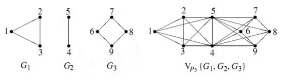
Considering the family of graphs $F=\{G_1,G_2,G_3\}$ as depicted in Figure 1 and the graph $G=P_3,$ the path of order 3, the generalized distance matrix $D_{\alpha }\left(H\right)$ of the joined union $H=P_3[G_1,G_2,G_3]$ is a block matrix of the form

$$\left(\begin{array}{ccc}{S}_1& J(1-\alpha )& 2J(1-\alpha )\\ J(1-\alpha )& S_2& J(1-\alpha )\\ 2J(1-\alpha )& J(1-\alpha )& S_3\end{array}\right),$$

where $S_i=\alpha (14I-2J+A\left(G_i\right))+2J-2I-A\left(G_i\right),i=1,3$ and $S_2=\alpha (10I-2J+A\left(G_2\right))+2J-2I+A\left(G_2\right).$

Since the adjacency spectrums of $G_1,G_2,G_3$ are $spe{c}_A\left(G_1\right)=\{{(-1)}^{\left[2\right]},2\},spe{c}_A\left(G_2\right)=\{-1,1\}$ and $spe{c}_A\left(G_3\right)=\{-2,0^{\left[2\right]},2\},$ respectively, then from Theorem 3, the generalized distance spectrum of H, consists of the eigenvalues $\left\{13\alpha -1^{\left[2\right]},14\alpha -2^{\left[2\right]},9\alpha -1,12\alpha \right\},$ also with the eigenvalues of the matrix

$$\left(\begin{array}{ccc}10\alpha +2& 2(1-\alpha )& 8(1-\alpha )\\ 3(1-\alpha )& 7\alpha +1& 4(1-\alpha )\\ 6(1-\alpha )& 2(1-\alpha )& 8\alpha +4\end{array}\right).$$

Therefore, $spe{c}_{D_{\alpha }}\left(H\right)=\left\{13\alpha -1^{\left[2\right]},14\alpha -2^{\left[2\right]},9\alpha -1,12\alpha ,16\alpha -4,\frac{9\alpha +11\pm \sqrt{81{\alpha }^2-202\alpha +137}}{2}\right\}.$

Note that, as $D_0\left(H\right)=D\left(H\right)$, then the distance spectrum of H is

$$spe{c}_D\left(H\right)=\left\{-1^{\left[2\right]},-2^{\left[2\right]},-1,0,-4,\frac{11\pm \sqrt{137}}{2}\right\}.$$

Also, as $D_{\frac{1}{2}}\left(H\right)=\frac{1}{2}{D}^Q\left(H\right)$, then the distance signless Laplacian spectrum of H is

$$spe{c}_{D^Q}\left(H\right)=\left\{8^{\left[2\right]},{10}^{\left[2\right]},{11}^{\left[2\right]},7,12,23\right\}.$$

References

- Barik, S.; Sahoo, G. On the distance spectra of coronas. Linear Multilinear Algebra 2017, 65, 1617–1628. [Google Scholar] [CrossRef]
- Barik, S.; Pati, S.; Sarma, B.K. The spectrum of the corona of two graphs. SIAM J. Discrete Math. 2007, 24, 47–56. [Google Scholar] [CrossRef]
- Cardoso, D.M.; de Freitas, M.A.; Martins, E.A.; Robbiano, M. Spectra of graphs obtained by a generalization of the join graph operation. Discrete Math. 2013, 313, 733–741. [Google Scholar] [CrossRef]
- Neumann, M.; Pati, S. The Laplacian spectra of graphs with a tree structure. Linear Multilinear Algebra 2009, 57, 267–291. [Google Scholar] [CrossRef]
- Shang, Y. Random lifts of graphs: Network robustness based on the Estrada index. Appl. Math. E-Notes 2012, 12, 53–61. [Google Scholar]
- Stevanović, D. Large sets of long distance equienergetic graphs. Ars Math. Contemp. 2009, 2, 35–40. [Google Scholar] [CrossRef]
- Cvetković, D.M.; Doob, M.; Sachs, H. Spectra of Graphs—Theory and Application; Academic Press: New York, NY, USA, 1980. [Google Scholar]
- Aouchiche, M.; Hansen, P. Distance spectra of graphs: A survey. Linear Algebra Appl. 2014, 458, 301–386. [Google Scholar] [CrossRef]
- Aouchiche, M.; Hansen, P. Two Laplacians for the distance matrix of a graph. Linear Algebra Appl. 2013, 439, 21–33. [Google Scholar] [CrossRef]
- Cui, S.Y.; He, J.X.; Tian, G.X. The generalized distance matrix. Linear Algebra Appl. 2019, 563, 1–23. [Google Scholar] [CrossRef]
- Alhevaz, A.; Baghipur, M.; Ganie, H.A.; Shang, Y. Bounds for the generalized distance eigenvalues of a graph. Symmetry 2019, 11, 1529. [Google Scholar] [CrossRef]
- Alhevaz, A.; Baghipur, M.; Ganie, H.A.; Shang, Y. On the generalized distance energy of graphs. Mathematics 2020, 8, 17. [Google Scholar] [CrossRef]
- Brouwer, A.E.; Haemers, W.H. Spectra of Graphs; Springer: New York, NY, USA, 2012. [Google Scholar]
- Schwenk, A.J. Computing the characteristic polynomial of a graph. In Graphs Combinatorics; Bary, R., Harary, F., Eds.; Lecture Notes in Mathematics; Springer: Berlin, Germany, 1974; Volume 406, pp. 153–172. [Google Scholar]
© 2020 by the authors. Licensee MDPI, Basel, Switzerland. This article is an open access article distributed under the terms and conditions of the Creative Commons Attribution (CC BY) license (http://creativecommons.org/licenses/by/4.0/).