Article

A Simplified Climate Change Model and Extreme Weather Model Based on a Machine Learning Method

1
GNSS Research Center, Wuhan University, Wuhan 430079, China
2
School of Civil Engineering, Wuhan University, Wuhan 430072, China
3
School of Civil and Environmental Engineering, University of Technology Sydney, Ultimo, NSW 2007, Australia
4
Huaibei Administration for Market Regulation, Huaibei 235000, China
*
Authors to whom correspondence should be addressed.
Symmetry 2020, 12(1), 139; https://doi.org/10.3390/sym12010139
Submission received: 8 December 2019 / Revised: 5 January 2020 / Accepted: 7 January 2020 / Published: 9 January 2020

Abstract

:
The emergence of climate change (CC) is affecting and changing the development of the natural environment, biological species, and human society. In order to better understand the influence of climate change and provide convincing evidence, the need to quantify the impact of climate change is urgent. In this paper, a climate change model is constructed by using a radial basis function (RBF) neural network. To verify the relevance between climate change and extreme weather (EW), the EW model was built using a support vector machine. In the case study of Canada, its level of climate change was calculated as being 0.2241 (“normal”), and it was found that the factors of CO2 emission, average temperature, and sea surface temperature are significant to Canada’s climate change. In 2025, the climate level of Canada will become “a little bad” based on the prediction results. Then, the Pearson correlation value is calculated as being 0.571, which confirmed the moderate positive correlation between climate change and extreme weather. This paper provides a strong reference for comprehensively understanding the influences brought about by climate change.

1. Introduction

Over the past hundred decades, global temperatures have been rapidly rising. According to the latest data from NASA, the long-term trend of global temperature rise has become more apparent, as is indicated in Figure 1. From 1880 to 2018, where the warmest ten years begin at 2015, and 2016 is the hottest year since 1880 [1,2]. However, the impacts of climate change (CC) are not just a rise in temperature. There is much scientific evidence showing that the effects brought by climate change are diverse, such as warming oceans, decreased snow cover, sea-level rise, ocean acidification, extreme events, etc. [3]. The negative influence of climate change seems to appear more and more prominent. It creates not only new risks and exacerbates existing vulnerabilities, but also offers various challenges to human health and safety, quality of life, and the rate of economic growth [4]. In order to prevent the further development of climate change, some scientific associations have studied the root causes of climate change and it is undeniable that human activities are the main factors [5]. However, there are still many factors that should be highlighted. Simply studying the relationship between certain natural phenomena and climate change cannot reflect the impact of climate change from a macro perspective. Therefore, a comprehensive study involving various influential factors is critically needed [6].
There is a large volume of published studies that have researched the influence of climate change. Some scientific methods have already been adopted in climate change research. Research using a process-oriented approach reveals the ecological response to recent climate change [7]. It discussed the phenology and physiology of organisms, the range and distribution of species, the composition of the community, and the dynamic characteristics of ecosystems. This confirms that climate change does have an influence on various species and human society, and it exposes a consistent mode of ecological change across the whole system [8]. Then, a scientific study on the sensitivity, potential impact, adaptability, and vulnerability of forests was conducted, which indicated that moderate increases in carbon dioxide concentration and temperature will promote forest growth and wood productivity in the short term. However, the enormous risks brought by extreme weather (EW) phenomena, such as drought and floods, is likely to reduce the wood productivity of the forest [9]. Another important finding has found that the impact of climate change on biological species is becoming more apparent than ever before. Using a climate envelope species distribution model to disclose the effect of climate change on wild crop relatives, 16–22% of the estimated species will go extinct in a specific migration scenario, and the range size of most species will reduce by over 50% [10]. In fact, the occurrence of climate change not only brings a huge challenge to the ecological environment and species diversity, but may also increase the spread of infectious diseases. This is because an essential consequence of climate change is global warming, and the rise of temperatures can accelerate the spread of some infectious diseases, such as the Ross River virus disease, which will likely threaten human health [11,12,13]. In addition, climate change is also closely related to community well-being, which suggests that the impact of climate change on human society is increasing [14]. Meanwhile, climate change adaptation policies caused by climate change also play an essential role in the stability of the country and society [15,16]. Obviously, climate change is no longer a matter of simple ecological environment change, but is also a primary issue related to social stability and national sustainable development.
However, the current impacts of climate change have not been quantified clearly. Most research approaches verify the existence of climate change using existing data and phenomena. It should be mentioned that the data on climate change factors are often small in magnitude [17,18]. Hence, the public is not sensitive to the effects of climate change. For instance, the 2019 United Nations Climate Change Conference had announced that the global average annual temperature rise rate is only 0.03 °C, a phenomenon called hiatus [1]; the small change rate of 0.03 °C can cause the public to mistakenly believe that climate change has stopped, and as such, the public will think that the government does not need to continue to put too much energy and money on the issues surrounding climate change. The lack of support of government work will bring certain risks to social stability, and the public’s misunderstanding of climate change will continue to exacerbate the negative impact of climate change. In addition, in some regions, the potential impact of climate change has been overlooked due to economic backwardness, and in other regions, the impact of climate change has been exaggerated because of the hype from media and other platforms. Having an unscientific understanding of climate change is useless for solving climate problems, since even if the real data reflected by climate change do not fluctuate greatly, its impact will not be small. The public needs to correctly understand the current level of climate change and its future developmental trends, and the gap between the real situation and the public’s imagination needs to be balanced. Therefore, research on quantifying the effects of climate change is essential for a sustainable future.
The purpose of this study is to achieve the coordination and symmetry between the micro research and the macro research, the complex climate and weather phenomena are integrated with scientific theories through analysis and modeling. First, providing a mathematical model of climate change that is able to be explained and comprehended. Second, the constructed extreme weather model is unique in its ability to quantify the effects of extreme weather conditions. Third, explaining the relevance between climate change and extreme weather. This research aims to provide a new way to understand the impact of climate change better.
The content structure is arranged as follows: Part 1 is a comprehensive introduction. Part 2 introduces the methods of constructing the climate change model and the extreme weather model. Part 3 provides the results and discussion, and the conclusion is given in Part 4.

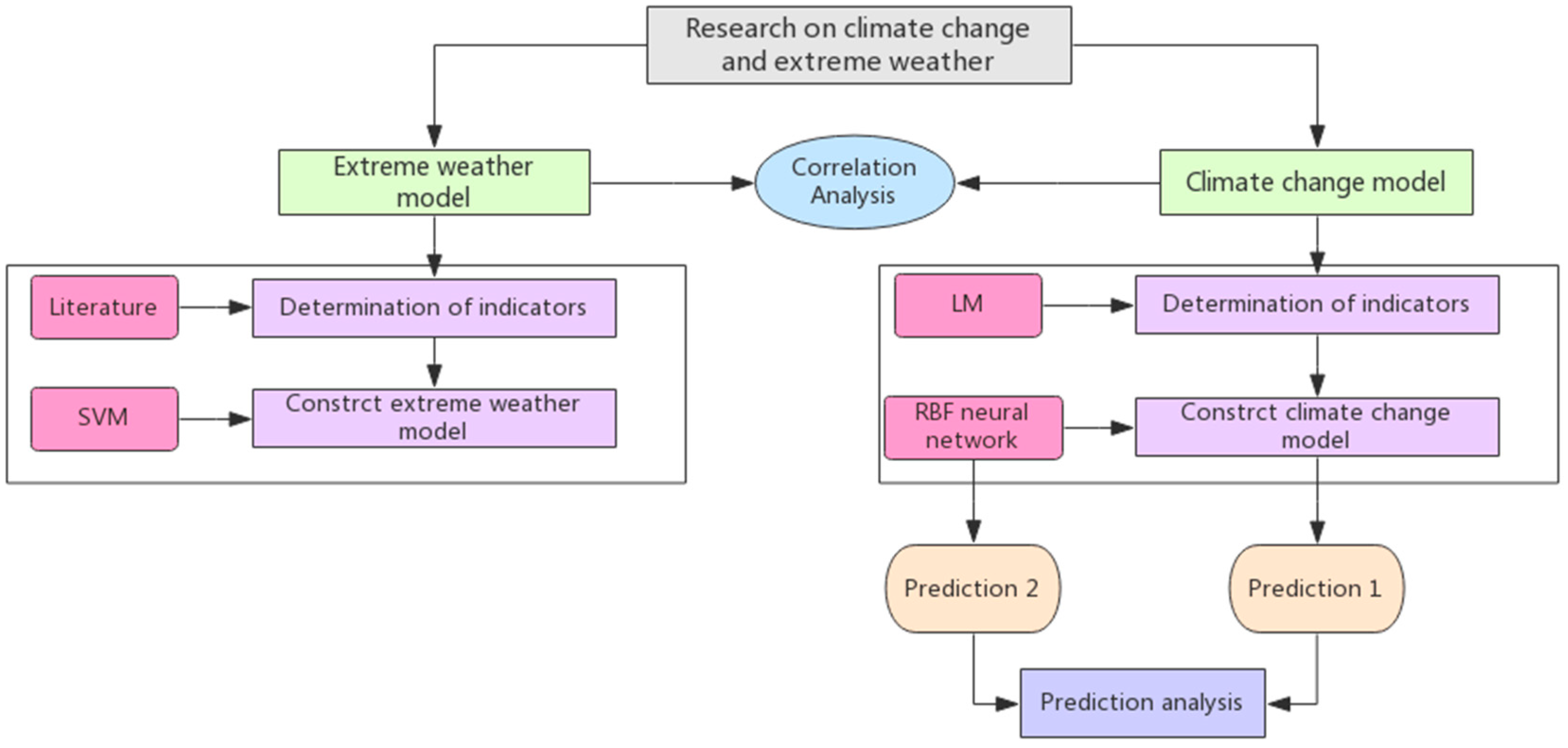
2. Materials and Methods

2.1. Assumptions

Some climate-related weather models usually involve many changeable factors. Some assumptions are put forward to make the model more scientific.
Hypothesis 1.
The trend of temperature changes is continuous all the time, and there is no sudden increase or decrease in temperature.
Hypothesis 2.
The official data obtained from the observatory is enough to represent the changes within the study area and the officially provided data is accurate.
Hypothesis 3.
The statistical data is reliable in terms of reflecting the true meaning of the indicator.
Hypothesis 4.
When discussing the temporal and spatial trends of temperature, the temporal and spatial variations of temperature are considered to be two relatively independent variables.
Hypothesis 5.
The original climate change system is a grey system. The selected impact indicators are independent of each other and there is no cross-impact or complex multi-collinearity.
Hypothesis 6.
The EW model can be decomposed into the sum of the extreme temperature model (TM) and the extreme precipitation model (PM). Additionally, the complex nonlinear relationships or other relationships that may exist between TM and PM are not considered.

2.2. Construct the Climate Change Model

In a prevailing view, a complete CC model should be capable of guiding the government and relevant policymakers toward clarifying the current climate status and possible future climate change trends [19]. Thus, the work toward obtaining a CC model can be divided into two parts: (1) determining the significant indicators and (2) constructing the CC model using some reliable mathematical methods. The value of the influence of climate change (C) is defined as the level of climate change, which belongs in the range 0–1. When the value of C is closer to 0, it means the state of the climate is more stable and better. When the value of C is closer to 1, it means the state of the climate is worse. Therefore, C can be defined as the following:
C = i = 1 n x i × q i + ε ,
where i is the ith impact indicator, i = 1, 2, …, 11, q i is the weight coefficient of the ith indicator, C i is the climate change value of the ith indicator, and adding the climate change values of all indicators gives the overall climate change value. x i is the normalized processed value of the ith index, which is obtained by mapping the index to the interval [0,1] after dimensionless processing. ε is the error term of the CC model. The expression of the important factor x i is given as follows:
x i = x x m i n x m a x x m i n .
In order to obtain the CC model, determining the indicators involved in the CC model should be completed at first.

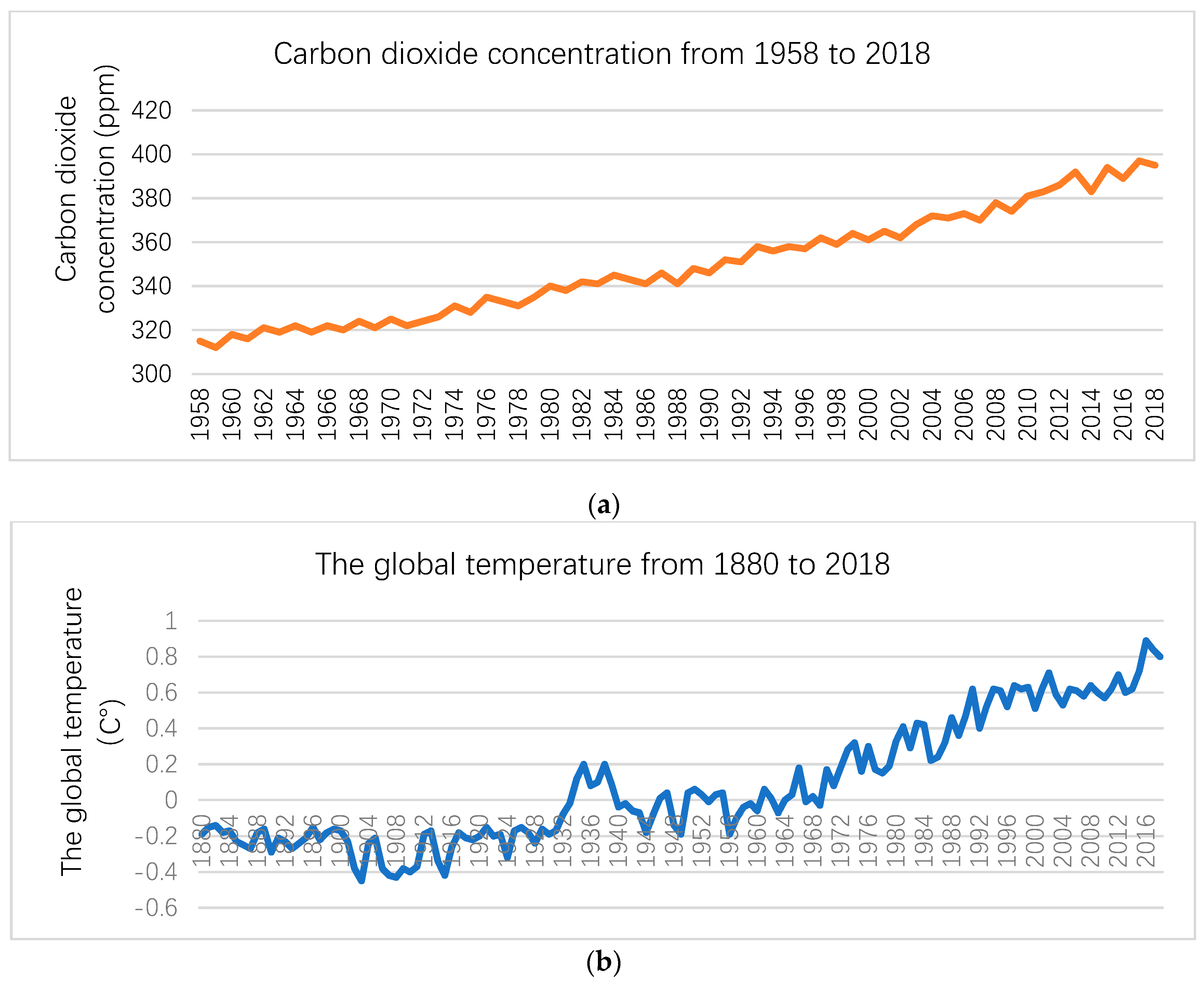
2.2.1. Determination of the Indicators

It is well accepted that there are numerous factors affecting climate change; however, this does not mean that each factor contributes significantly to climate change. To determine the important factors contributing to climate change, Laplacian eigenmapping (LM) was used as a nonlinear dimensionality reduction technique is adopted to facilitate the establishment of the CC model.
LM is a graph-theory-based method. It maps the randomly distributed points in space through analyzing the similarity between neighboring structures to obtain the data shape in low-dimensional space [20]. According to the local neighbor relationship existing in the high-dimensional space, the data set of the local neighbor relationship in the low-dimensional area is obtained.
The graph is composed of nodes and edges. The edge represents the value information. The degree of the node is the number of edges passing through the point. The degree of node i is the sum of the weights of all edges passing through the node. The definition matrix D is a diagonal matrix whose primary oblique element value is the degree of the node.
d i = j w i j , D = [ d 1 0 0 d n ] ,
where d i is the weight of the edge between nodes i and j .
In this study, the directed graph of the LM was applied, which is a semi-positive definite matrix. All the eigenvalues are non-negative real numbers. The transform of dimensionality reduction is obtained by decomposing the eigenvalues of the LE matrix.
The selected data set x 1 , x 2 ,   , x n are the vectors of space vector R l , and the space vector of the expected dimensionality reduction is defined as R m , m l . M is a manifold embedded in R l . The steps involved in applying the LM are as follows.
1. Establish the adjacency relationship of the construction diagram
If the distance between the sample points of x i and x j is small, an edge can be made for x i and x j . When judging the distance between two sample points, the criterion is the neighbor rule. If node i is in the nearest n neighbor node sets of the node j , then the nodes of i and j are considered to be close. If there are five nodes, the possible relationship can be described as shown in Figure 2, thereby the relationship between nodes can be determined.
2. Calculate the weight of the edge
If node i exists on the edge of node j , it means that the two nodes are connected and the weights of the edges w i j between the two nodes are given by:
w i j = e x p ( x i x j 2 t ) ,
where t is a constant. If two nodes are unconnected, then w i j = 0 .
After getting the weight of each edge, then the directed graph can be obtained.
3. Feature mapping
Based on the directed graph, calculate the Laplacian matrix and solve the generalized eigenvalues and eigenvector values:
L f = λ D f ,
where L represents the Laplacian matrix, f is the generalized matrix, and λ is the eigenvalue.
If the solution of the generalized matrix is f 0 , f 1 ,   , f k 1 , the feature vector values are sorted in ascending order to obtain:
0 = λ 0 λ 1     λ k 1 .
If the eigenvalue of the point is zero, remove the point. Subsequently, the eigenvectors of the remaining points are constructed into the final projection matrix. The data is mapped into the low-dimensional space, thereby the dimensionality reduction processing of the indicator is complete.

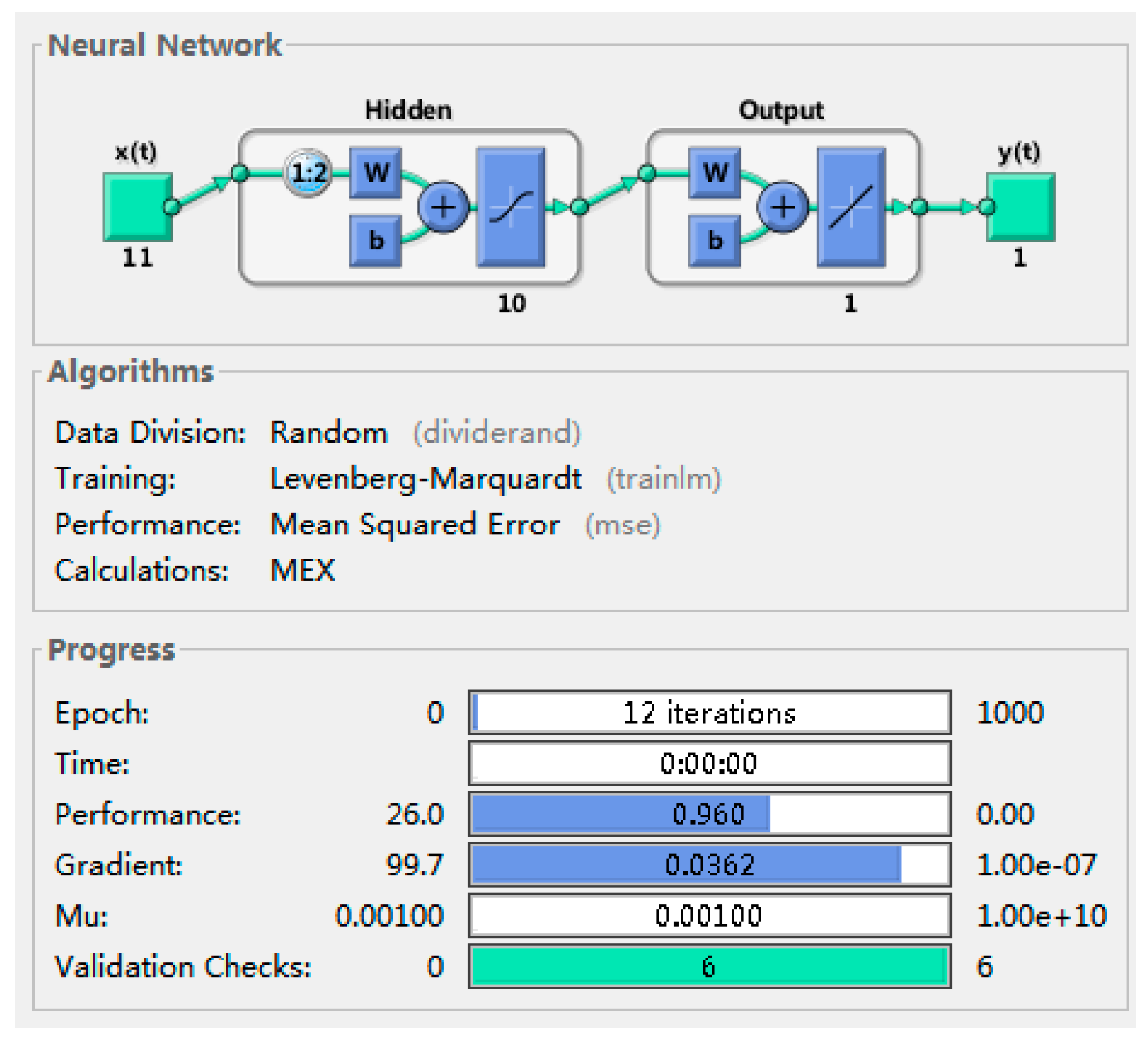
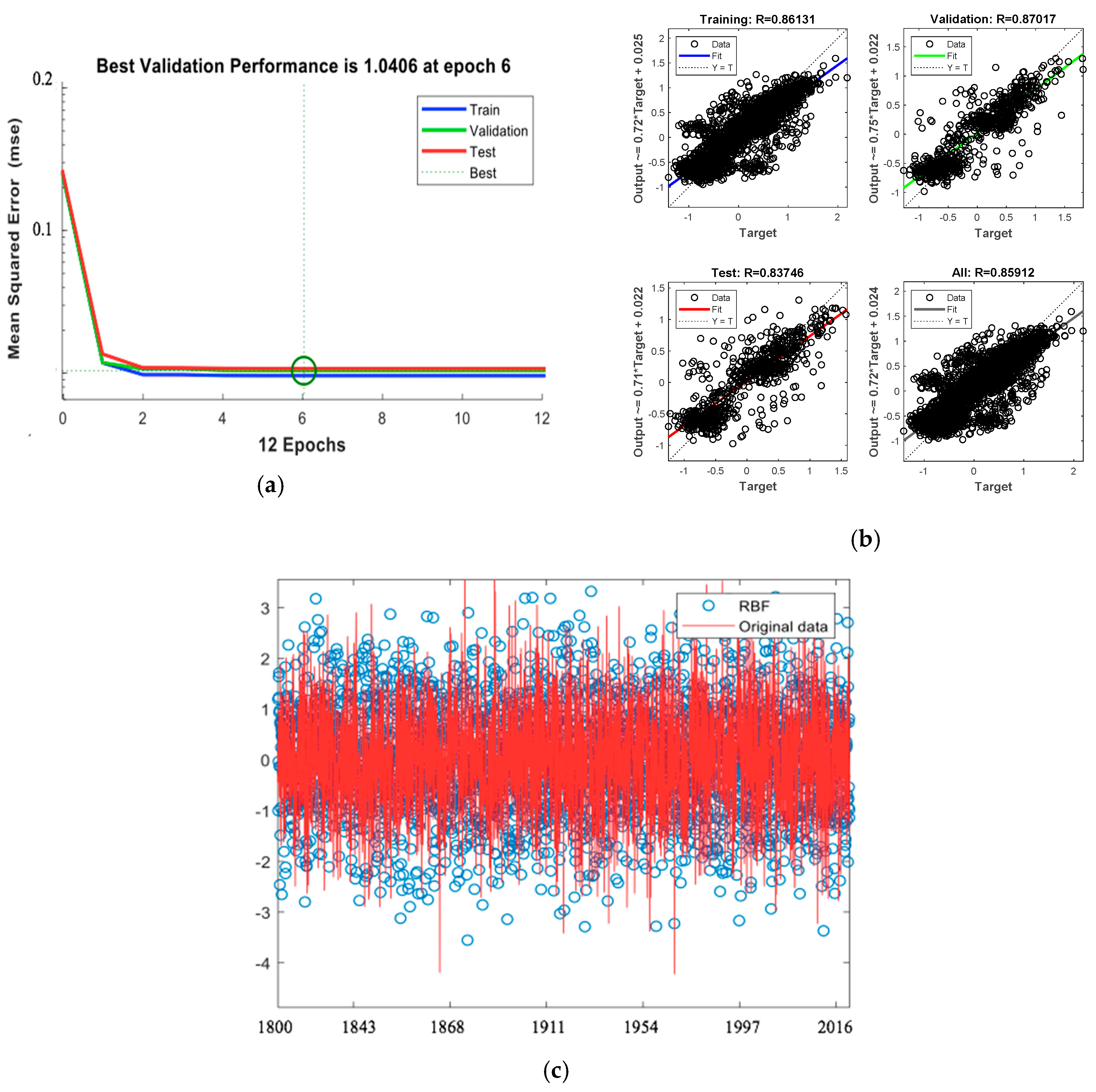
2.2.2. Climate Model Based on a Radial Basis Function Neural Network

Inspired by the work of predecessors, a radial basis function (RBF) neural network is adopted to get the weight coefficient of each indicator. It is worth noting that the RBF neural network is suitable for managing the issues of weight connections. The relationship between the input vector and the output vector can be confirmed without the requirement of weight connections [21]. There is a linear assumption between the hidden layer and the output layer, namely that the output of the network is linear for tunable parameters. Thus, the speeds of learning and training are promoted in a way, and the learning rate is rather low. When the amount of involved data is quite large, the dominating advantage of the RBF neural network becomes clear. The significant steps of the RBF neural network are shown below.
(1) The determination of parameters
1. Identify the initial input vector, output vector, and expected output vector:
X = [ x 1 , x 2 , , x n ] , Y = [ y 1 , y 2 , , y q ] , O = [ o 1 , o 2 , , o q ] T ,
here X is the input vector and n represents the nth input layer. Y is the output vector, and O is the expected output vector. q is the qth output layer.
2. Initialize weights between the hidden layer and the output layer:
W k = [ w k 1 , w k 2 , , w k p ] T , ( k = 1 , 2 , , q ) ,
where p is the pth hidden layer.
Based on center initialization theory, the weight initialization method from the hidden layer to the output layer is expressed below:
W k j = m i n k + j m a x k m i n k q + 1 ,
where m i n k is the minimum value of all expected outputs in the kth output neuron in the training set and m a x k is the maximum value of all expected outputs of the kth output neuron in the training set.
3. Initialize the central parameters of each neuron in the hidden layer
The initial value of the central parameter of the RBF neural network is given below:
c j i = m i n i + m a x i m i n i 2 p + ( j 1 ) m a x i m i n i   p ,
where p is the total number of neurons in the hidden layer and j = 1 ,   2 ,   ,   p .
4. Initialize the width vector
The width vector affects the range of the action of neurons regarding input information; the smaller the width, the narrower the shape of the action function of the corresponding hidden layer neurons. Its function is as follows:
d j i = d f 1 N k = 1 N ( x i k c j i ) ,
where d f is the width adjustment coefficient; its value is less than 1. The function of d f is to realize the ability to perceive and respond to local information easily and accurately.
(2) Calculate the output value, z j , of the jth neuron in the hidden layer:
z j = exp ( X C j D j 2 ) , j = 1 ,   2 ,   , p ,
C j = [ c j 1 , c j 2 , , c j n ] ,
D j = [ d j 1 , d j 2 , , d j n ] T ,
where C j is the central vector in the hidden layer of the jth neuron. It is composed of the jth neuron in the hidden layer corresponding to the central component of all neurons in the input layer. D j is the width vector of the jth neuron in the hidden layer corresponding to C j .
(3) Calculate the output of neurons in the output layer:
Y = [ y 1 , y 2 , , y q ] T ,
y k = j = 1 p w k j z j ,   k = 1 ,   2 ,   , q .
(4) Calculate the weight coefficient
The training method for the weight parameters of the RBF neural network is the gradient descent method. The central, width, and adjusting weight parameters are adjusted to the best value by learning through adaptation, and the iterative calculation is as follows:
W k j ( t ) = W k j ( t 1 ) η E W k j ( t 1 ) + α [ W k j ( t 1 ) W k j ( t 2 ) ] ,
c j i ( t ) = c j i ( t 1 ) η E c j i ( t 1 ) + α [ c j i ( t 1 ) c j i ( t 2 ) ] ,
d j i ( t ) = d j i ( t 1 ) η E d j i ( t 1 ) + α [ d j i ( t 1 ) d j i ( t 2 ) ] ,
where W k j ( t ) is the adjustment weight between the kth output neuron and the jth hidden layer neuron in the tth iteration calculation. c j i ( t ) is the adjustment weight between the jth output neuron and the ith hidden layer neuron in the tth iterative calculation. d j i ( t ) is the width corresponding to the centre c j i ( t ) .
Then, the evaluation function of the RBF neural network is constructed as follows:
E = 1 2 l = 1 N k = 1 q ( y l k O l k ) 2 ,
where E represents the evaluated result of the RBF neural network, O l k is the expected output value of the kth output neuron in the input sample l , and y l k is the network output value of the kth output neuron in the input sample l .
(5) Calculate the R M S of the network output:
R M S = i = 1 N k = 1 q ( O l k y l k ) q N .
If RMSε, the network training is finished. Otherwise, retrain the network from step 3.

2.3. Construct the Extreme Weather Model

Recently, global warming has been intensifying, but local extreme weather frequently occurs, which makes many people think that global warming has already stopped. The paradox is whether there is a conflict between the climate change model and the extreme weather model. Therefore, it is necessary to carry out deeper research on extreme weather. Furthermore, another goal of establishing an EW model is to separate the factors that can explain extreme weather from a series of disordered extreme weather indicators.

2.3.1. Determination of the Indicators

In this study, the EW model only covers extreme temperature conditions and extreme precipitation conditions. According to Kaas and Frich [22], the requirements for extreme weather indicators are “weak extremes, low noise, and more reliable.” In the previous study of extreme weather, the extreme value threshold method is usually used to define whether a weather phenomenon is extreme. If the threshold value is exceeded, the weather condition is considered to be an extreme weather event. The threshold value is set according to the existing literature, studies, and standards published on the government website. Hence, this study finally selected 13 indicators that can be used to describe extreme weather. The selected indicators and the corresponding threshold values can be seen in Table 1.

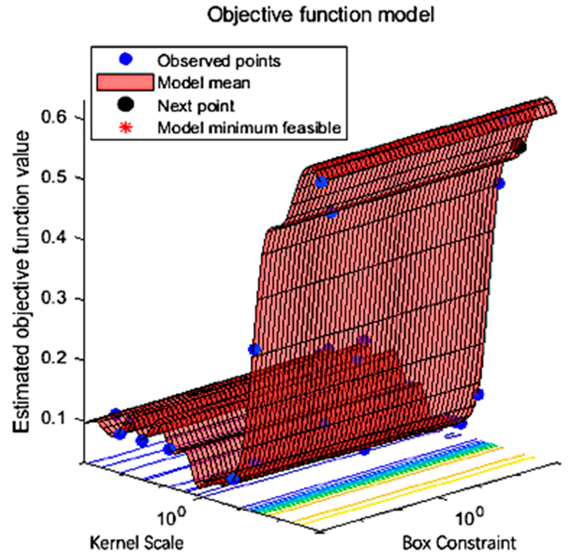
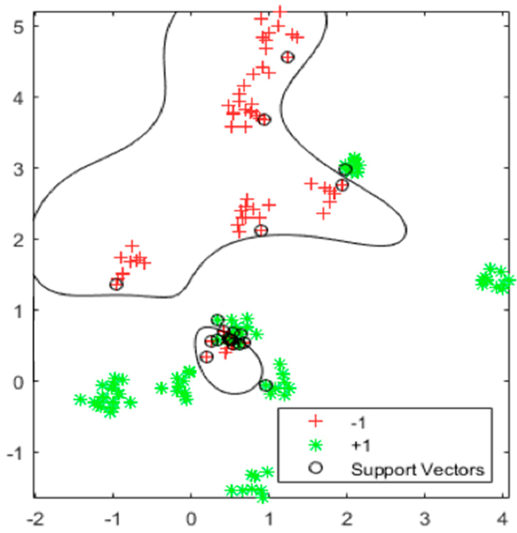
2.3.2. Extreme Weather Model Based on Support Vector Machine

The primary purpose of establishing the extreme weather model was to separate the factors that can explain extreme weather from a series of disordered extreme weather indicators and assign corresponding weights to these explanatory variables to define extreme weather. A support vector machine (SVM) method was adopted to establish the EW model. Different from prior perceptron models, a SVM can classify a distance hyperplane more accurately, especially the point closest to the hyperplane distance. The core element of the SVM method is to keep the spots near the hyperplane away from the hyperplane. Then, maximize the interval such that the classification points are on both sides of the respective support vectors to achieve an optimized classification effect [23].
Assume the hyperplane has the form w T x + b , where it is required that a point close to the hyperplane moves far from the hyperplane. This can be described as follows:
m a x γ = y ( w T x + b ) w 2   ( i = 1 ,   2 , , m ) s . t . y i ( w T x i + b ) = γ ( i ) γ ,
where x is the input vector, w is the weight vector, b is the bias, and γ is the function interval, which is used to determine whether the index classification is correct. At the same time, in order to unify the conditions, a constraint condition is added to the normal vector w , and γ is defined to measure the precise distance between the hyperplane and the observed value. In this part, the constraint function y i ( w T x i + b ) is defined as being 1, and therefore Equation (22) can be simplified to:
m a x γ = 1 w 2 s . t . y i ( w T x i + b ) 1   ( i = 1 ,   2 , , m ) .
Since the maximization problem of 1 w 2 is equivalent to the minimization problem of 1 2 w 2 2 , the optimization function of SVM is equivalent to Equation (24):
m i n 1 2 w 2 2 s . t . y i ( w T x i + b ) 1   ( i = 1 ,   2 , , m ) .
The objective function 1 2 w 2 2 is convex, so the Lagrangian function can be used to solve the optimal norm problem. The mathematical form of the Lagrangian function is shown as follows:
L ( w , b , α ) = 1 2 ω 2 2 i = 1 m α i [ y i ( ω T x i + b ) 1 ] , α i 0 ,
where α i represents the optimal coefficient of the hyperplane.
Subsequently, optimization goals can be simplified as m i n   m a x   L ( ω , b , α ) by deriving the partial derivatives of w and b , respectively.
L w = 0 w = i = 1 m α i y i x i , L b = 0 I ˙ = 1 m α i y i = 0 .
Based on Equation (26), the relationship between w and α can be determined. Therefore, the optimization function ψ ( α ) can be defined:
ψ ( α ) = m i n   L ( ω , b , α ) , ψ ( α ) = i = 1 m α i 1 2 i = 1 ,   j = 1 m α i α J ˙ y i y j x i T x j .
Owing to ψ ( α ) only having a relationship with α , the problem of solving the objective function ψ ( α ) can be transformed to obtain the solution α :
m a x 1 2 i = 1 m α i j = 1 m α i α j y i y j ( x i x j ) i = 1 m α i s . t .   i = 1 m α i y i = 0 , α i 0 ,   i = 1 ,   2 , , m
The solution process of Equation (28) requires the use of the sequential minimal optimization algorithm to obtain the corresponding values of α* and ω* [24]. Through the above processes, all points can be classified on the side of their respective support vectors. A linear ε insensitive loss function is selected to allow for error minimization. Then, the RBF neural network is used to regress the SVM. Due to the different parameter values set in the software, the regression function shape obtained is quite different [25]. Therefore, it remains a need to learn and train the sample multiple times, the best combination of parameters can be obtained eventually, and the regression parameters of the SVM can be obtained as well.

3. Results and Discussion

3.1. Data

In this study, Canada was the targeted country. Historical data on weather across Canada can be found at http://climate.weather.gc.ca/historical_data/search_historic_data_e.html. In fact, there are many climatic stations in every administrative region of Canada. In this study, due to the influence of regional differences on the research results, stations in every administrative region were selected. Additionally, due to the impact of factors, such as the scale of different climate stations, equipment accuracy, management, etc., the quality of data between each site varied a lot. Therefore, the quality of the data provided by the station is taken into consideration during station selection. The selected climate stations are shown in Figure 3 and Table 2.
Initially, data preprocessing on the original data was performed. First, all data was imported into the MATLAB (R2019a) software and the properties of the data strip with incomplete data was set, allowing for the existence of null values. The data obtained contained noise and clutter, and therefore data mining technology was used to perform cleaning, integration, conversion, discretization, and reduction on the filtered data. As is indicated in Figure 4, the data fluctuated greatly, and there were abnormal points. The maximum variance of some data was 2.1 when the deviation test was performed.
Then, the data attributes were verified. The types of the data were digital, the interval was set to [−30, 20], and the length of the value ranged was up to one decimal place. Outliers were identified as points that were more than two standard deviations away from the mean of a given attribute. The clustering adjusted the existing deviation correction. The processed result is shown in Figure 5, where it is apparent that the processed data is smooth and stable.

3.2. The Climate Change Model

Using the existing literature and official government documents as a reference, some original indicators affecting climate change can be selected [26,27]. However, the quality of the information varies greatly, therefore information from the academic literature is dominant, which is supplemented by information obtained from other channels. First, when acquiring indicators on the basis of a range of information sources, the indicators should be sufficiently independent, and its corresponding data needs to be available. Then, the frequency of each indicator should be counted. The initial index selection results are shown in Table 3. Owing to the large workload, only some of official and literature sources are shown below.
It should be mentioned that although 17 original indicators were determined, the significance of each indicator was ambiguous. Therefore, it was necessary to use scientific mathematical methods to identify the important indicators, and only indicators that had a significant impact on the overall result were retained in the climate change model. First, Stata 15.0 and MATLAB (R2019a) software were applied to extract the corresponding data. Then, LM was used to select the indicators with significant contributions. In addition, the climate was viewed as a grey system with multivariate interaction; by considering the uncertainty and greyness of the system, the RBF neural network was used to determine the influence weight coefficient of each index, and the CC model was finally obtained.

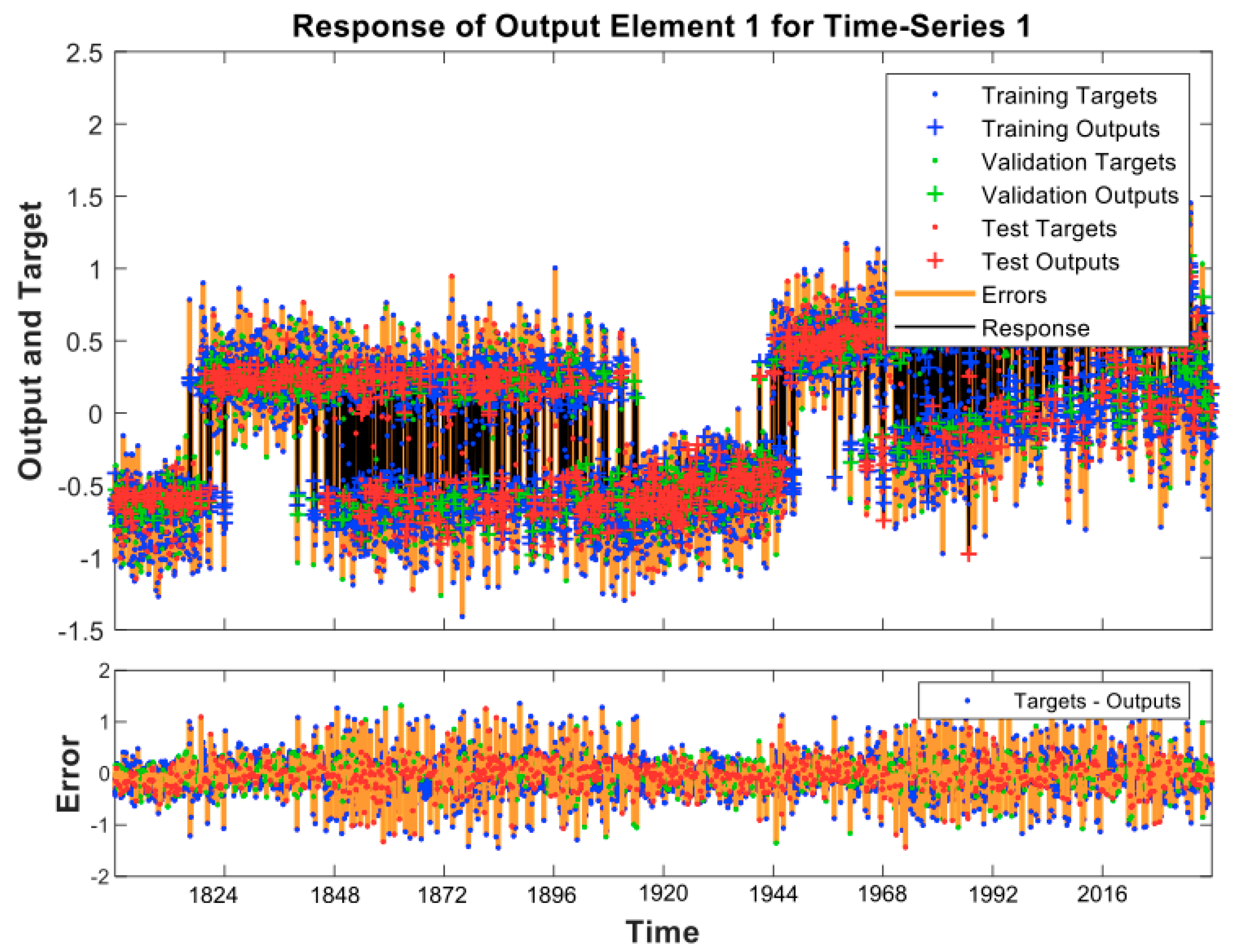
3.2.1. Determination of the Climate Change Model

LM was applied to recognize the significant indicators. As the 17 original indicators were confirmed, the adjacency relationship of the construction diagram was subsequently established, and the conceptual diagram is shown in Figure 6.
Using MATLAB software to conduct the feature mapping, the points with an eigenvalue of zero were removed to construct the final projection matrix using the eigenvectors of the remaining points. The dimension reduction processing of the indicator was completed when the data was mapped in a low-dimensional space. The results are shown in Figure 7, the original data was scattered randomly in three-dimensional space, and the ordered data in two-dimensional space was obtained after the dimensionality reduction process. Finally, the identified important factors are represented in Table 4.
The RBF neural network was applied after all the indicators were determined. The processes of adopting the RBF neural network are shown as follows.
1. Preparation of data
The MATLAB software was adopted to conduct the RBF neural network. The input and output variables for the RBF neural network were the selected 11 indicators. The eligible data of 11 indicators were put into MATLAB. Due to a large amount of data, considering the limitation of computer processing efficiency, the data was first subjected to fast Fourier transform (FFT) processing. Then, the data was standardized [54]. Each indicator belonged to the interval [−1, 1]. The feature vector of the FFT processed sequence was later used as the training sequence. In accordance with successful experience [55] and multiple attempts, in this paper, 60% of the data was used for training, 20% of data was used for testing, and 20% of data was used for validation. It was confirmed that the above proportion has the best training performance for the subsequent processes. Furthermore, the maximum number of training times was set to 1000, the learning precision was 0.01, and the model automatically generated the number of hidden nodes. The maximum threshold of the indicator was 1, and the minimum threshold was −1. First, a pre-experiment was undertaken to determine the appropriate number of neurons. Through several experiments, the number of neurons in the hidden layer was set to 10, R 2 0.9 , and the performance of the model reached 0.96. When the number of neurons was greater than 10, although the training effect was better in a way, the testing effect was poor. Therefore, it was reasonable to set the number of neurons to 10. The residual and the average residual were required to be less than 0.05, and the number of iterations was 12. The specific structure of the RBF neural network is shown in Figure 8.
2. Analysis of the error
The root mean square error (RMSE) is a primary index to evaluate the level of error [56]. The RMSE output using MATLAB software, as is indicated in Figure 9, quickly decreases and then tended infinitely toward zero after the second iteration, which suggests that the model worked well, and the model performance was optimal at the sixth iteration (1.0406). Then, the reliability R was output as R ≥ 0.85912, which indicates that the model was very reliable. In the end, after comparing the training data with the pre-retained verification set data, it can be seen that the two data sets were quite close. Hence, it was confidently confirmed that the training results were very stable.
3. End training
After the RBF neural network with preset parameters passed the error test, the model operation result could be output. Furthermore, there was a “weight connection one” between the input layer and the hidden layer, and a “weight connection two” between the hidden layer and the model calculation output layer; therefore, these two connections should be handled further. To verify the performance of the RBF neural network, confirmation of the response of the outputted 11 variables was required. As shown in Figure 10, the training, test, and validation sets were close to each other, and the consistency shown by the three data sets was indicated by a low level of error. Therefore, the results of the operation of the RBF neural network were acceptable, and as such, the training could be terminated.
The weight connection one and the weight connection two were collated and analyzed. After calculating some relevant parameters according to Equation (10), the CC model could be obtained as follows:
c = 0.1132 x 1 0.0965 x 2 + 0.1031 x 3 + 0.0905 x 4 + 0.1163 x 5 + 0.0814 x 6 + 0.0681 x 7 + 0.0502 x 8 + 0.1311 x 9 + 0.0171 x 10 + 0.1321 x 11 + v = 1 4 ε v ,
where ε v is the vth error term: ε 1 represents the error caused by the Pacific decadal oscillation, ε 2 represents the instability error caused by the El Niño phenomenon, ε 3 represents the instability error caused by the La Niña phenomenon, and ε 4 represents the sum of other possible instability errors.
Since there is no general standard for measuring the magnitude of climate change, the level of climate change needed to be defined after obtaining the CC model. This paper selected 189,742 sample data from different regions of the world from 1800 to 2019 to calculate the climate change value. Then, using statistical techniques for statistical analysis, the climate change values were given corresponding climate levels, as defined in Table 5.
Averaging the known values of all the indicators of 13 stations, they were put into the established climate change model. Consequently, the current climate change level of Canada was calculated to be 0.2241. This indicates the level of Canada’s climate change is normal, which is a very intuitive indication given that climate change in Canada is still acceptable.
Through analyzing the CC model, it can be found that the amount of ice coating had a negative effect on climate change, and “the average temperature” and “global carbon dioxide concentration” were significant factors. Their relationship was interpreted under the circumstance of the global climate condition, as indicated in Figure 11, where global temperature and carbon dioxide concentration both showed a significant upward trend from 1880 to 2018. Then, the average temperature of Canada from 1981 to 2019 was considered to obtain the temperature change rate (temperature load) and the average temperature of each region. When the temperature load was more significant than zero, the temperature had an upward trend [57,58]. All temperature loads and average temperatures are visualized on the map of Canada shown in Figure 12.
In Figure 12, the temperature loads of the research areas were greater than zero. The normal state of Canada’s climate change is a microcosm of global climate change which indicates the positive correlation between temperature and carbon dioxide. Furthermore, the area with the most significant temperature load was NU (0.0037), and the temperature loads of the southeast coastal areas were all great than zero, indicating that the region will continue to experience warming in the future. In the area of the western coast, the temperature of BC was abnormally high, which may be related to the occurrence of the El Niño and La Niña phenomena in recent years. Furthermore, the fluctuation of the temperature load was significant, which also showed a clear trend of upward fluctuation in three-dimensional space.
Also, the contribution of sea surface temperature (SST) to climate change was quite large [59]. After obtaining the data of SST (data provided by the NOAA/OAR/ESRL PSD, Boulder, Colorado, USA, from their website at https://www.esrl.noaa.gov/psd/), the temperature profile of the SST worldwide from 1800 to 2019 was produced. As indicated in Figure 13, the larger the yellow area in the figure, the wider the coverage of the SST high-temperature range. Before 1880, the high-temperature center of the SST was concentrated around the area of the eastern Pacific Ocean, and then the central area of the high temperature continuously expanded [34]. The area with the highest SST was concentrated in the central area of the Pacific Ocean and the Indian Ocean. In the eastern part of Africa and the southern part of Asia and the Indian Ocean, the average SST has increased from [22,27] to [27,30]. The increase in SST near the west coast of Canada was consistent with the rise in the average temperature in the coastal area, thereby the contribution of SST to climate change cannot be neglected.

3.2.2. Predictions of the CC Model

A prediction of the possible trend of climate change can provide more useful guiding information, and it can help the public, government, and policymakers have a holistic concept of climate change. Meanwhile, to verify the predicted performance of the established model, two different predictions were conducted, and the prediction differences were compared in detail.
First, the CC model was used to obtain the climate change values C from 1800 to 2019. C was used as the input variable of the RBF neural network. The maximum number of training times was set to 500 times, the learning precision was 0.01, and the model automatically generated the number of hidden nodes. The prediction time was from 2019 to 2044 (the next 25 years). The maximum and minimum thresholds of the indicator were 1 and −1, respectively. After several pre-experiments, the number of neurons was set to 7 and the number of iterations was 9. When the residual and the average residual was less than 0.05, the training was terminated; the resulting prediction result is called “Prediction 1.”
Second, the original data set was divided as a test set, a training set, and a verification set. The test set was processed by the RBF neural network directly. The maximum number of training times was set to 1000, the learning precision was 0.01, the model automatically generated the number of hidden nodes, and the forecast time was the next 25 years. The maximum and minimum thresholds of the indicator were 1 and −1, respectively. The number of hidden layer neurons and iterations were both set to 10, and the performance of the model was the best (1.002) under the above settings. When the average residual was less than 0.05, the training was terminated. The RBF neural network was used to output the initial predicted values, then the CC model was applied to process the above values to output the final predicted results (“Prediction 2”). The results of the two predictions are shown in Figure 14.
It can be seen that the climate level will gradually transfer from “normal” to “a little bad.” In 2025, the global climate level will break through the normal level, and the future climate change will develop in the direction of “a little bad” in the long term. Additionally, the forecast result of “Prediction 1” was close to that of “Prediction 2”, indicating that the CC model was reliable and had a good applicability. In 2053, “Prediction 1” shows a downward trend, while “Prediction 2” shows a sudden upward trend. The possible reason for this phenomenon is the scale effect caused by the data. Thereby the CC model’s prediction stability remained for 34 years. Since climate change is a quite complex phenomenon, through the limited amount of data, there will be numerous uncertainties in predicting changes over decades. The subsequent optimization of the model can be conducted by improving the stable prediction performance of the model in the long term.

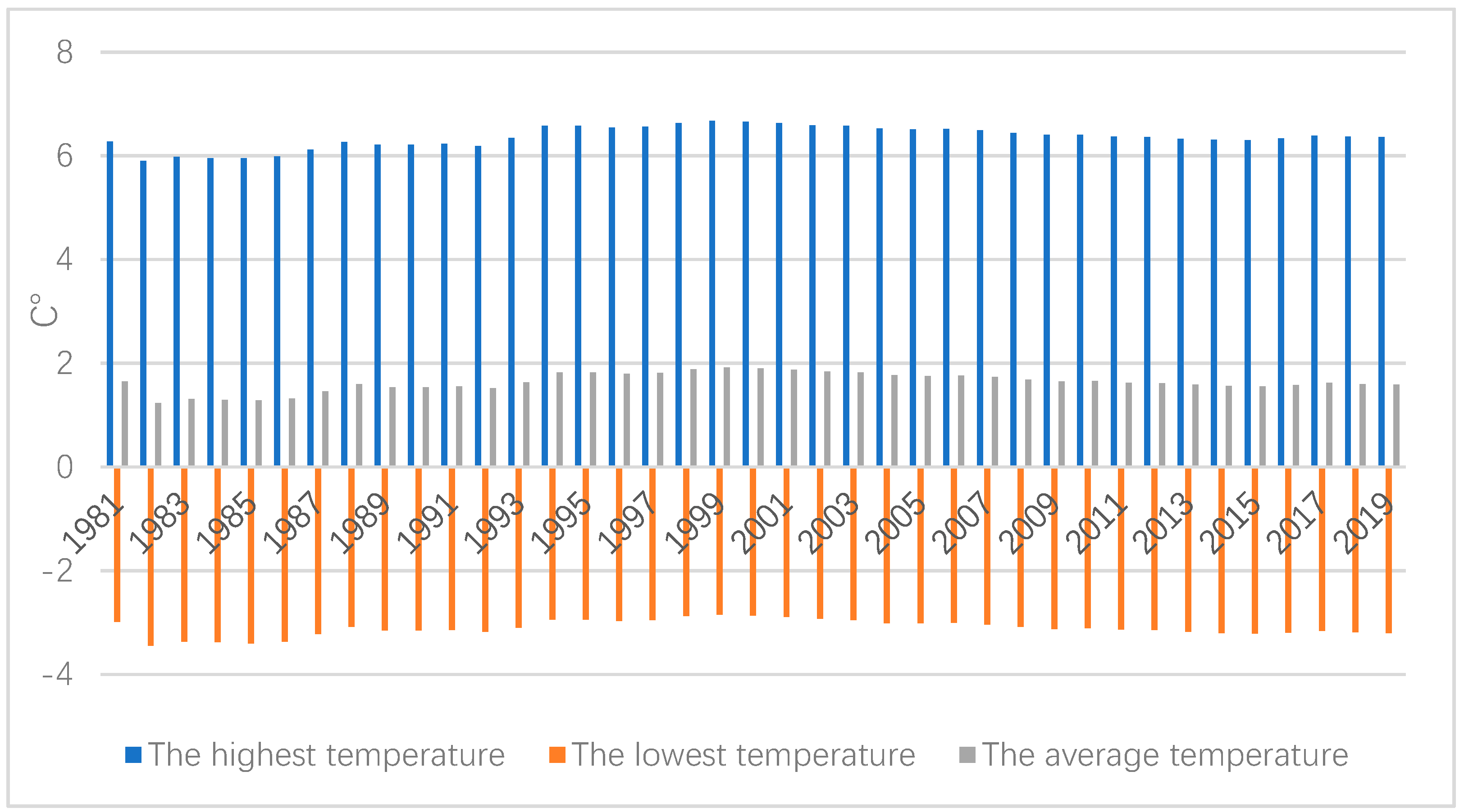
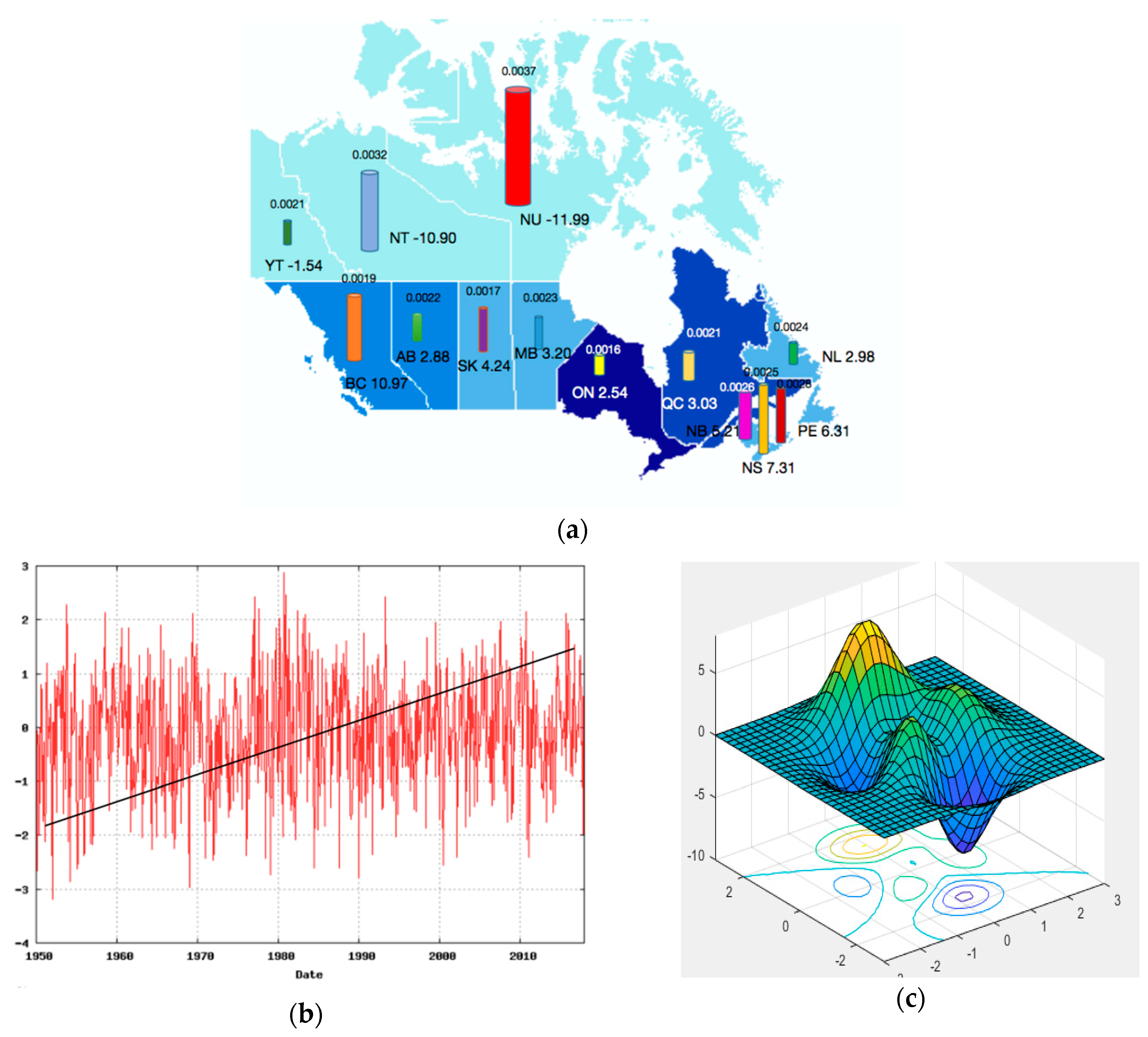
3.3. The Extreme Weather Model

In this study, we used a SVM to construct the EW model. The modelling process was divided into the following parts.
1. Indicator classification
(1) Input data
The data of thirteen indicators were averaged in the Canadian grid model and then all indicators were projected into the interval of [−2, 5] in the plane. As shown in Figure 15, red indicates the precipitation indicators and green indicates the temperature indicators.
(2) Generate a scatter plot
Since the values of a single category were difficult to classify and did not have a general law, the index was projected to [−2, 6] under each category. Figure 16 shows that the red reference points were very close to the green reference points. In order to facilitate the division and avoid the problem that the classification boundary was not clear due to a large amount of data, this study only generated ten regular distribution data points based on each category. The length of each category indicator was 244 × 12 months = 2928 months.
(3) Mark the category
A vector file was created to mark the class of each point as a label for each vector. The vector took a value of −1 or 1, indicating that the class belonged to precipitation or temperature.
(4) Cross-validation
Cross-validation means that most of the samples were modelled, and a small number of samples were used to predict the established model and to solve the forecast error of a small number of samples [60]. To reduce the error of cross-validation, Bayesian optimization was used to reduce the loss due to cross-validation.
(5) Calculate the objective function value
The objective function values were calculated under the constraints of the box constraint and the kernel function. The observation point was projected onto the hyperplane, where the nonlinear hyperplane is shown as the red area in Figure 17.
(6) Classify indicators
After the processing of SVM, all indicators could be divided into two categories: precipitation indexes and temperature indexes, which are the red and green points shown in Figure 18, respectively. Through the classification, a clear division of the indicator attributes was prepared for SVM regression processing.
2. The regression of the SVM
This paper proposes a calculation method based on the extreme weather fluctuation value (JD) in the unit grid to reflect extreme weather fluctuations. The value of JD is between 0 and 1. The closer the JD value is to 1, the greater the weather fluctuations and the more extreme the weather conditions. The definition of JD is as follows:
y i = h i min { h i } max { h i } min { h i } , J D 1 = 7 y i ( i = 1 7 ( h i h ¯ ) 3 2 n σ 3 × h i h ¯ σ + 1 ) 1 3 × e 0.0001 i + δ 1 , J D 2 = 6 y i ( i = 8 13 ( h i h ¯ ) 3 2 n σ 3 × h i h ¯ σ + 1 ) × e 0.0001 i + δ 2 ,
where h i is the original value; y i is the processed value; max   { h i } and min { h i } are the maximum and minimum values of the indicator data set under the category, respectively; y i indicates the normalized result of all indicators; JD1 indicates the temperature indexes; JD2 indicates the precipitation indexes; n indicates the total number; σ indicates the standard deviation of the indicator; and e 0.0001 i represents a time-varying exponent term. δ 1 represents the disturbance term of the temperature and δ 2 represents the disturbance term of the precipitation, both of which are regarded as normally distributed random noise.
Using the processed indicators as inputs, with an output value of JD, the indicator data set from 1800 to 2009 was selected as the training sample set and the indicator data set from 2010 to 2019 was used as the verification set. The linear ε insensitive loss function was selected for controlling the error minimization, and the radial basis kernel function was applied in the SVM regression. Finally, the regression parameters of SVM could be obtained. The extreme temperature model and the extreme precipitation model are shown below:
y 1 = 0.0176 h 1 0.0361 h 2 + 0.1073 h 3 + 0.0144 h 4 + 0.1334 h 5 + 0.1621 h 6 + 0.105 h 7 + δ 1 , y 2 = 0.0126 h 8 + 0.1763 h 9 + 0.1019 h 10 + 0.0104 h 11 + 0.0133 h 12 + 0.1327 h 13 + δ 2 ,
where δ 1 is the sum of possible noise associated with temperature and δ 2 is the sum of possible noise related to precipitation.
Furthermore, ample data was calculated to obtain the distribution of the extreme temperature values and extreme precipitation values. Using statistical analysis, the interval classifications of the extreme temperature indicators and the extreme precipitation indicators were found and are shown in Table 6.

3.4. Correlation Analysis

The occurrence of a climate change hiatus is confusing and creates the illusion that climate change has stopped [61]. In January 2019, two-thirds of the United States and Canada had large hail events, and there was unusual extreme cold weather. Hence, many people held a view that global warming has stopped and the government does not have to spend too much energy and expenses on global-warming-related work [62,63]. In order to help the public better understand the relationship between global warming and local extreme cold weather, this study selected the Selkirk Fortress region of Canada as an example to analyze its correlation. The reason for choosing the Selkirk Fortress region is that it has obvious characteristics of extreme weather, and the data for climate change and extreme weather of the Selkirk Fortress region is available and complete. Through the above discussion, the CC model and the EW model were related to different factors. The key interface was the time when analyzing its correlation. The study period was from 1990 to 2018, and the statistics of h1h7 from September to January in the Selkirk Fortress area were selected.
Through applying the CC model and the EW model, the climate change values and extreme cold weather values could be obtained. Then, the Pearson correlation value ρ C T . was chosen to judge the relevance relationship, where 1 ρ C T 1 . When ρ C T is positive, it indicates that there is a positive correlation. Otherwise, it suggests that there is a negative correlation [64]. The magnitude of the correlation is presented in Table 7.
Due to the large amount of data, this paper used the SPSS 17.0 to calculate the correlation value. After importing the obtained values into the SPSS software, the value of ρ C T was found to be 0.571, which indicates that there was a moderate positive correlation. This means that when local extreme cold weather occurs frequently, climate change will become active; as a result, the extreme cold weather will become more serious, and the climate change value will increase as well. It worth noting that the typical manifestation of progressive climate change is global warming. Therefore, while the extreme local cold occurs, global warming may occur; therefore, the local extreme cold and global warming are not contradictory. The public should have confidence in the government’s policy decisions and make their contributions through energy conservation and emissions reductions throughout their daily lives. In the context of abnormal global climate change, focusing on long-term benefits is far more important than short-term benefits, which inevitably requires the joint efforts of people all over the world.

3.5. Discussion

The work surrounding climate change and extreme weather is quite complex and tough, which is because climate and weather are the result of a combination of spatial factors at a particular time. Climate impacts have been identified, but their magnitude is still vague. This research aimed to provide reliable evidence for the impact of current climate change and extreme weather, and provides the public with a dialectical perspective on the current climate and weather conditions.
The work in this research was conducted by establishing climate change and extreme weather models. As is indicated in Figure 19, the research could not only evaluate current conditions, but also predicted the change of future climate change. Furthermore, the relationship between climate change and extreme weather were recognized through the scientific method.
In the case study, Canada was selected as our research object. The work was divided into three parts: (1) constructing the climate change model, then making a prediction; (2) constructing the extreme weather model; and (3) conducting a correlation analysis. When constructing CC model, Stata and MATLAB software were used to obtain the corresponding data, and LM was used to determine 11 significant indicators. Then, the CC model was established on the basis of an RBF neural network. It was found that the current climate change level of Canada is 0.2241, which indicates that the level of Canada’s climate change is normal on the whole. Meanwhile, the amount of ice coating had a negative effect on climate change, and “the average temperature” and “global carbon dioxide concentration” were quite significant factors, and the contribution of SST was recognized as well. Furthermore, a prediction of the possible trend of climate change can provide more useful guidance information, and considering differences in the model performance, two prediction methods were conducted at the same time, which were from the CC model and RBF neural network. It was found that the global climate level will break through the normal level in 2025 and the future climate change will develop in the direction of “a little bad” in the long term. Additionally, the forecast result indicated that the CC model is reliable and has good applicability. However, the prediction ability of the CC model is up to 34 years. When constructing the extreme weather model, due to the local and targeted characteristics of the indicators in the EW model, reliable precipitation and temperature indicators were extracted from prior literature. Then, the EW model is constructed on the basis of a SVM and the JD algorithm. In the final correlation analysis, the Selkirk Fortress region of Canada was selected as the research area due to its obvious extreme characteristics. After extracting corresponding data of its indicators from 1990 to 2018, the Pearson correlation value was selected to measure the correlation between climate change and extreme weather. The results showed that there was a moderate positive correlation; therefore, even if local extreme weather is frequent, global warming will continue as well. The above result is also strong evidence that can explain the apparent contradiction between local extreme cold and global warming. As the above results are studied from the perspective of a macro average, if the model is applied to a narrower area, the Pearson value will be larger.
In fact, some similar machine learning models have already been adopted in researching the issues regarding climate change. For example, support vector machines (SVMs), artificial neural networks (ANNs), and generalized regression neural network (GRNN) have been applied to assess the impact of climate change on the above-ground biomass. However, due to the existence of systematic errors and the lack of consideration of time series, the uncertainty of the model is large [65]. Another study adopted an ANN method to determine the influence of climate drivers on sand-deposition in semi-arid regions [66]. ANN was also adopted to provide globally consistent estimates of precipitation [67]. However, the shortcoming of the above research is that the output model may be less accurate due to insufficient training times. The biggest difference between this study and other studies lies in the following three points: (1) The model is more stable. The RBF neural network can rapidly improve the performance of the model according to the number of training times. The prediction ability of the CC model based on the RBF neural network and LM can perform better. Furthermore, the model established in this paper can directly extract the attributes of the original data and give feedback information, and the computer operation efficiency of the CC and EW models were significantly improved, and the inefficient and high-error processing status caused by the large amount of data was solved. (2) The model considers the time series of the data. The data used in this study was the complete data set with a long time series to make full use of the original attributes of the data and avoid the occurrence of data distortion caused by multi-model processing. (3) This research is more comprehensive. All possible factors affecting climate change and extreme weather were considered in the research, instead of focusing on at most a few factors. Therefore, the macro guidance of this research is more significant.
The CC and EW models were established on the basis of relevant machine learning theory, which was quite an innovative method. The forecasting time scale of the CC model was found to be 34 years, which is realizable and stable in a way. The main reason for the limitation was the variability of the climate change system and the scale effect of the data. Future scholars can optimize CC models through other neural network theories. Furthermore, it should be mentioned that the research in this article was based on the macro average state, so it may be inconsistent with local special cases, where the large research area and scattered data are the most likely reasons. To improve the local application performance of the model, future scholars can improve the model performance by continuously optimizing the parameters.

4. Conclusions

This research aimed to help the public better understand the current situation of climate change and provide useful information for the government. The research was conducted by constructing the CC and EW models. In the research area of Canada, the CC model was constructed using LM and a RBF neural network, and the current climate change level of Canada was calculated to be 0.2241, which indicates that the overall level of climate change of Canada is still normal. However, the climate change level of Canada will transfer from “normal” to “a little bad” in 2025 on the basis of the prediction result. Furthermore, it was found that the CO2 level, average temperature, and SST were significant factors to climate change. In order to figure out the relationship between climate change and extreme weather, the EW model was established using an SVM. Additionally, the EW model could be divided into a TM model and PM model. Then, the Pearson correlation analysis was applied, and its value was calculated to be 0.571, which confirmed that there was a moderate positive correlation. This research provides guidance for government policy formulation and correct public awareness, which is not only conducive to the government’s better allocation of fiscal expenditure through more reasonable policies, but also helps the public to make their own efforts through having a correct perception. Climate change can only be solved through the joint efforts of the government and the public.
However, there are some areas where the above established models can be improved. The prediction accuracy of the CC model lasts for 34 years. Beyond this predicted time threshold, the model exhibited instability. In addition, when establishing the extreme weather model, it was assumed that the extreme temperature model and the extreme precipitation model were independent of each other. Actually, there are complex nonlinear relationships, which may have a certain impact on the accurate application of the model. Future scholars can optimize the model by improving the prediction stability of the model in the long term and process the temperature and precipitation data directly to obtain a more accurate mathematical model. This paper provides a new perspective for the public to understand climate change and extreme weather while providing a useful reference for governments and relevant policymakers.

Author Contributions

Project administration, X.R.; software, X.R.; methodology, L.L.; writing—original draft, L.L.; resources, Y.Y.; investigation, Z.X.; validation, S.Y.; supervision, W.D.; formal analysis, M.R. All authors have read and agreed to the published version of the manuscript.

Funding

This research received no external funding.

Acknowledgments

The inspiration source for this paper is problem E in the Huawei Cup Mathematical Modeling, which gave us new perspectives on climate change and extreme weather. It also provided us with a lot of motivation and encouragement to make our efforts toward a beautiful and peaceful world, calling on everyone to pay attention to climate change.

Conflicts of Interest

The authors declare no conflict of interest.

References

  1. Heymann, M. The climate change dilemma: Big science, the globalizing of climate and the loss of the human scale. Reg. Environ. Chang. 2019, 19, 1549–1560. [Google Scholar] [CrossRef]
  2. Hulme, M. Why We Disagree about Climate Change: Understanding Controversy, Inaction, and Opportunity. Response Prog. Hum. Geogr. 2011, 35, 136–138. [Google Scholar]
  3. Wang, B.; Hong, G.; Cui, C.-Q.; Yu, H.; Murty, T. Comprehensive analysis on China’s National Climate Change Assessment Reports: Action and emphasis. Front. Eng. Manag. 2019, 6, 52–61. [Google Scholar] [CrossRef]
  4. Mazo, J. Climate Change Impacts in the United States: The Third National Climate Assessment. Survival 2014, 56, 175–183. [Google Scholar] [CrossRef]
  5. Wan, H.; Zhang, X.B.; Zwiers, F. Human influence on Canadian temperatures. Clim. Dyn. 2019, 52, 479–494. [Google Scholar] [CrossRef]
  6. Elisa, P.; Alessandro, P.; Andrea, A.; Silvia, B.; Mathis, P.; Dominik, P.; Manuela, R.; Francesca, T.; Voglar, G.E.; Tine, G.; et al. Environmental and climate change impacts of eighteen biomass-based plants in the alpine region: A comparative analysis. J. Clean. Prod. 2020, 242, 12. [Google Scholar] [CrossRef]
  7. Harper, E.T. Ecological Gentrification in Response to Apocalyptic Narratives of Climate Change: The Production of an Immuno-political Fantasy. Int. J. Urban Reg. Res. 2019. [Google Scholar] [CrossRef] [Green Version]
  8. Walther, G.R.; Post, E.; Convey, P.; Menzel, A.; Parmesan, C.; Beebee, T.J.C.; Fromentin, J.M.; Hoegh-Guldberg, O.; Bairlein, F. Ecological responses to recent climate change. Nature 2002, 416, 389–395. [Google Scholar] [CrossRef]
  9. Lindner, M.; Maroschek, M.; Netherer, S.; Kremer, A.; Barbati, A.; Garcia-Gonzalo, J.; Seidl, R.; Delzon, S.; Corona, P.; Kolstrom, M.; et al. Climate change impacts, adaptive capacity, and vulnerability of European forest ecosystems. For. Ecol. Manag. 2010, 259, 698–709. [Google Scholar] [CrossRef]
  10. Jarvis, A.; Lane, A.; Hijmans, R.J. The effect of climate change on crop wild relatives. Agric. Ecosyst. Environ. 2008, 126, 13–23. [Google Scholar] [CrossRef]
  11. Dennis, S.; Fisher, D. Climate Change and Infectious Diseases: The Next 50 Years. Ann. Acad. Med. Singap. 2018, 47, 401–404. [Google Scholar] [PubMed]
  12. McVea, D.; Copes, R.; Galanis, E. Climate change and infectious disease in Canada and BC. Br. Columbia Med. J. 2018, 60, 463–464. [Google Scholar]
  13. Smith, E. The Effect of Potential Climate Change on Infectious Disease Presentation. JNP J. Nurse Pract. 2019, 15, 405–409. [Google Scholar] [CrossRef]
  14. Bryce Kennedy, P.G. Measuring Progress on Climate Change Adaptation: Lessons from the Community Well-Being Analogue. J. Integr. Disaster Risk Manag. 2015, 5, 115–134. [Google Scholar] [CrossRef]
  15. Dolšak, N.; Prakash, A. The Politics of Climate Change Adaptation. Annu. Rev. Environ. Resour. 2018, 43, 317–341. [Google Scholar] [CrossRef] [Green Version]
  16. Purdon, M. Advancing Comparative Climate Change Politics: Theory and Method Introduction. Glob. Environ. Politics 2015, 15, 1–26. [Google Scholar] [CrossRef]
  17. Palchik, N.A.; Moroz, T.N.; Miroshnichenko, L.V.; Artamonov, V.P. Crystal Chemistry of Carbonates and Clay Minerals from Bottom Sediments of Okhotskoe Sea as an Indicator of Climate Change. In Proceedings of the 9th Geoscience Conference for Young Scientists, Ekaterinburg, Russia, 5–8 February 2018; pp. 161–168. [Google Scholar]
  18. Lee, J.S.; Choi, H.I. Comparative Analysis of Flood Vulnerability Indicators by Aggregation Frameworks for the IPCC’s Assessment Components to Climate Change. Appl. Sci. 2019, 9, 2321. [Google Scholar] [CrossRef] [Green Version]
  19. Sundaralingam, P. The Science of Climate Change. World Lit. Today 2019, 93, 74. [Google Scholar] [CrossRef]
  20. Hu, R.J.; Ratner, K.; Ratner, E.; Miche, Y.; Bjork, K.M.; Lendasse, A. ELM-SOM plus: A continuous mapping for visualization. Neurocomputing 2019, 365, 147–156. [Google Scholar] [CrossRef]
  21. Bagheri, V.; Uromeihy, A.; Aghda, S.M.F. A Comparison Among ANFIS, MLP, and RBF Models for Hazard Analysis of Rockfalls Triggered by the 2004 Firooz Abad-Kojour, Iran, Earthquake. Geotech. Geol. Eng. 2019, 37, 3085–3111. [Google Scholar] [CrossRef]
  22. Kaas, E.; Frich, P. Diurnal temperature-range and cloud cover in the nordic countries-observed trends and estimates for the future. Atmos. Res. 1995, 37, 211–228. [Google Scholar] [CrossRef]
  23. Cortes, C.; Vapnik, V. Support-vector networks. Mach. Learn. 1995, 20, 273–297. [Google Scholar] [CrossRef]
  24. Nagashzadeghan, M.; Shirzadi, M. Building Energy Optimization Using Sequential Search Approach for Different Climates in Iran. Int. J. Renew. Energy Res. 2015, 5, 210–216. [Google Scholar]
  25. Zeng, S.W.; Hu, H.G.; Xu, L.H.; Li, G.H. Nonlinear Adaptive PID Control for Greenhouse Environment Based on RBF Network. Sensors 2012, 12, 5328–5348. [Google Scholar] [CrossRef] [Green Version]
  26. Boles, W.C. The Science and Politics of Climate Change in Steve Waters’ The Contingency Plan. J. Contemp. Drama Engl. 2019, 7, 107–122. [Google Scholar] [CrossRef]
  27. Bui, H.X.; Maloney, E.D. Mechanisms for Global Warming Impacts on Madden-Julian Oscillation Precipitation Amplitude. J. Clim. 2019, 32, 6961–6975. [Google Scholar] [CrossRef]
  28. Kim, G.Y.; Lee, S. Prediction of extreme wind by stochastic typhoon model considering climate change. J. Wind Eng. Ind. Aerodyn. 2019, 192, 17–30. [Google Scholar] [CrossRef]
  29. Hawkins, L.R.; Rupp, D.E.; McNeall, D.J.; Li, S.H.; Betts, R.A.; Mote, P.W.; Sparrow, S.N.; Wallom, D.C.H. Parametric Sensitivity of Vegetation Dynamics in the Triffid Model and the Associated Uncertainty in Projected Climate Change Impacts on Western US Forests. J. Adv. Model. Earth Syst. 2019, 11, 2787–2813. [Google Scholar] [CrossRef] [Green Version]
  30. Hanittinan, P.; Tachikawa, Y.; Ram-Indra, T. Projection of hydroclimate extreme indices over the Indochina region under climate change using a large single-model ensemble. Int. J. Climatol. 2019. [Google Scholar] [CrossRef]
  31. Sakalli, A. Sea surface temperature change in the mediterranean sea under climate change: A linear model for simulation of the sea surface temperature up to 2100. Appl. Ecol. Environ. Res. 2017, 15, 707–716. [Google Scholar] [CrossRef]
  32. Colucci, R.R.; Guglielmin, M. Climate change and rapid ice melt: Suggestions from abrupt permafrost degradation and ice melting in an alpine ice cave. Prog. Phys. Geogr. 2019, 43, 561–573. [Google Scholar] [CrossRef]
  33. Kobler, U.G.; Schmid, M. Ensemble modelling of ice cover for a reservoir affected by pumped-storage operation and climate change. Hydrol. Process. 2019, 33, 2676–2690. [Google Scholar] [CrossRef]
  34. Carton, J.A.; Ding, Y.N.; Arrigo, K.R. The seasonal cycle of the Arctic Ocean under climate change. Geophys. Res. Lett. 2015, 42, 7681–7686. [Google Scholar] [CrossRef]
  35. Kumar, K.R.; Attada, R.; Dasari, H.P.; Vellore, R.K.; Abualnaja, Y.O.; Ashok, K.; Hoteit, I. On the Recent Amplification of Dust Over the Arabian Peninsula During 2002–2012. J. Geophys. Res. Atmos. 2019, 1124, 13220–13229. [Google Scholar] [CrossRef] [Green Version]
  36. Akinyoola, J.A.; Ajayi, V.O.; Abiodun, B.J.; Ogunjobi, K.O.; Gbode, I.E.; Ogungbenro, S.B. Dynamic response of monsoon precipitation to mineral dust radiative forcing in the West Africa region. Model. Earth Syst. Environ. 2019, 5, 1201–1214. [Google Scholar] [CrossRef] [Green Version]
  37. Burdejova, L.; Tobolkova, B.; Polovka, M. Effects of Different Factors on Concentration of Functional Components of Aronia and Saskatoon Berries. Plant Foods Hum. Nutr. 2019. [Google Scholar] [CrossRef]
  38. Alexander, P.M.; Tedesco, M.; Koenig, L.; Fettweis, X. Evaluating a Regional Climate Model Simulation of Greenland Ice Sheet Snow and Firn Density for Improved Surface Mass Balance Estimates. Geophys. Res. Lett. 2019, 46, 12073–12082. [Google Scholar] [CrossRef] [Green Version]
  39. Tapiador, F.J.; Sanchez, E.; Romera, R. Exploiting an ensemble of regional climate models to provide robust estimates of projected changes in monthly temperature and precipitation probability distribution functions. Tellus Ser. A Dyn. Meteorol. Oceanol. 2009, 61, 57–71. [Google Scholar] [CrossRef]
  40. Dai, A.G.; Zhao, T.B.; Chen, J. Climate Change and Drought: A Precipitation and Evaporation Perspective. Curr. Clim. Chang. Rep. 2018, 4, 301–312. [Google Scholar] [CrossRef]
  41. Lombardo, F.T.; Ayyub, B. Approach to Estimating Near-Surface Extreme Wind Speeds with Climate Change Considerations. ASCE ASME J. Risk. Uncertain. Eng. Syst. Part A Civ. Eng. 2017, 3, 11. [Google Scholar] [CrossRef]
  42. Saha, U.; Chakraborty, R.; Maitra, A.; Singh, A.K. East-west coastal asymmetry in the summertime near surface wind speed and its projected change in future climate over the Indian region. Glob. Planet. Chang. 2017, 152, 76–87. [Google Scholar] [CrossRef]
  43. Illy, T. Near-surface wind speed changes in the 21st century based on the results of Aladin-Climate regional climate model. Idojaras 2017, 121, 161–187. [Google Scholar]
  44. Leffler, A.J.; Beard, K.H.; Kelsey, K.C.; Choi, R.T.; Schmutz, J.A.; Welker, J.M. Cloud cover and delayed herbivory relative to timing of spring onset interact to dampen climate change impacts on net ecosystem exchange in a coastal Alaskan wetland. Environ. Res. Lett. 2019, 14, 10. [Google Scholar] [CrossRef] [Green Version]
  45. Coates, S.J.; Davis, M.D.P.; Andersen, L.K. Temperature and humidity affect the incidence of hand, foot, and mouth disease: A systematic review of the literature—A report from the International Society of Dermatology Climate Change Committee. Int. J. Dermatol. 2019, 58, 388–399. [Google Scholar] [CrossRef]
  46. Kleynhans, E.; Terblanche, J.S. Complex interactions between temperature and relative humidity on water balance of adult tsetse (Glossinidae, Diptera): Implications for climate change. Front. Physiol. 2011, 2, 74. [Google Scholar] [CrossRef] [Green Version]
  47. Terrenoire, E.; Hauglustaine, D.A.; Gasser, T.; Penanhoat, O. The contribution of carbon dioxide emissions from the aviation sector to future climate change. Environ. Res. Lett. 2019, 14, 12. [Google Scholar] [CrossRef]
  48. Chen, X.Z.; Liu, X.D.; Liu, Z.Y.; Zhou, P.; Zhou, G.Y.; Liao, J.S.; Liu, L.Y. Spatial clusters and temporal trends of seasonal surface soil moisture across China in responses to regional climate and land cover changes. Ecohydrology 2017, 10, 12. [Google Scholar] [CrossRef]
  49. Li, Y.; Su, T.; Sheng, L.; Qiang, P.; Zhao, B. Study of a high-precision pulsar angular position measuring method. Mod. Phys. Lett. B 2018, 32, 1850355. [Google Scholar] [CrossRef]
  50. Harrison, D.E.; Larkin, N.K. Darwin sea level pressure, 1876-1996: Evidence for climate change? Geophys. Res. Lett. 1997, 24, 1779–1782. [Google Scholar] [CrossRef]
  51. Reader, M.C.; Plummer, D.A.; Scinocca, J.F.; Shepherd, T.G. Contributions to twentieth century total column ozone change from halocarbons, tropospheric ozone precursors, and climate change. Geophys. Res. Lett. 2013, 40, 6276–6281. [Google Scholar] [CrossRef] [Green Version]
  52. Jankovic, A.; Podrascanin, Z.; Djurdjevic, V. Future climate change impacts on residential heating and cooling degree days in Serbia. Idojaras 2019, 123, 351–370. [Google Scholar] [CrossRef] [Green Version]
  53. Shi, Y.; Gao, X.J.; Xu, Y.; Giorgi, F.; Chen, D.L. Effects of climate change on heating and cooling degree days and potential energy demand in the household sector of China. Clim. Res. 2016, 67, 135–149. [Google Scholar] [CrossRef] [Green Version]
  54. Zhang, Y.W.; Gong, C.L.; Fang, H.; Su, H.; Li, C.N.; Da Ronch, A. An efficient space division-based width optimization method for RBF network using fuzzy clustering algorithms. Struct. Multidiscip. Optim. 2019, 60, 461–480. [Google Scholar] [CrossRef] [Green Version]
  55. Tian, Z.D.; Li, S.J.; Wang, Y.H. A prediction approach using ensemble empirical mode decomposition-permutation entropy and regularized extreme learning machine for short-term wind speed. Wind Energy 2019. [Google Scholar] [CrossRef]
  56. Willmott, C.J.; Matsuura, K. Advantages of the mean absolute error (MAE) over the root mean square error (RMSE) in assessing average model performance. Clim. Res. 2005, 30, 79–82. [Google Scholar] [CrossRef]
  57. Royer, D.L.; Berner, R.A.; Park, J. Climate sensitivity constrained by CO2 concentrations over the past 420 million years. Nature 2007, 446, 530–532. [Google Scholar] [CrossRef]
  58. Stanghellini, C.; Bontsema, J.; de Koning, A.; Baeza, E.J. An Algorithm for Optimal Fertilization with Pure Carbon Dioxide in Greenhouses. In International Symposium on Advanced Technologies and Management Towards Sustainable Greenhouse Ecosystems: Greensys 2011; Kittas, C., Katsoulas, N., Bartzanas, T., Eds.; ISHS: Leuven, Belgium, 2012; Volume 952, pp. 119–124. [Google Scholar]
  59. Huber, M.; Sloan, L.C. Climatic responses to tropical sea surface temperature changes on a “greenhouse” Earth. Paleoceanography 2000, 15, 443–450. [Google Scholar] [CrossRef] [Green Version]
  60. Kim, D.; Kang, S.; Cho, S. Expected margin-based pattern selection for support vector machines. Expert Syst. Appl. 2020, 139, 112865. [Google Scholar] [CrossRef]
  61. Winslow, L.A.; Leach, T.H.; Rose, K.C. Global lake response to the recent warming hiatus. Environ. Res. Lett. 2018, 13, 5. [Google Scholar] [CrossRef]
  62. Zheng, B.; Chevallier, F.; Yin, Y.; Ciais, P.; Fortems-Cheiney, A.; Deeter, M.N.; Parker, R.J.; Wang, Y.L.; Worden, H.M.; Zhao, Y.H. Global atmospheric carbon monoxide budget 2000-2017 inferred from multi-species atmospheric inversions. Earth Syst. Sci. Data 2019, 11, 1411–1436. [Google Scholar] [CrossRef] [Green Version]
  63. Le Quere, C.; Andrew, R.M.; Friedlingstein, P.; Sitch, S.; Pongratz, J.; Manning, A.C.; Korsbakken, J.I.; Peters, G.P.; Canadell, J.G.; Jackson, R.B.; et al. Global Carbon Budget 2017. Earth Syst. Sci. Data 2018, 10, 405–448. [Google Scholar] [CrossRef] [Green Version]
  64. Liu, X.S. A probabilistic explanation of Pearson’s correlation. Teach. Stat. 2019, 41, 115–117. [Google Scholar] [CrossRef]
  65. Wu, C.Y.; Chen, Y.F.; Peng, C.H.; Li, Z.C.; Hong, X.J. Modeling and estimating aboveground biomass of Dacrydium pierrei in China using machine learning with climate change. J. Environ. Manag. 2019, 234, 167–179. [Google Scholar] [CrossRef] [PubMed]
  66. Buckland, C.E.; Bailey, R.M.; Thomas, D.S.G. Using artificial neural networks to predict future dryland responses to human and climate disturbances. Sci. Rep. 2019, 9, 3855. [Google Scholar] [CrossRef] [PubMed] [Green Version]
  67. Nguyen, P.; Ombadi, M.; Sorooshian, S.; Hsu, K.; AghaKouchak, A.; Braithwaite, D.; Ashouri, H.; Thorstensen, A.R. The PERSIANN family of global satellite precipitation data: A review and evaluation of products. Hydrol. Earth Syst. Sci. 2018, 22, 5801–5816. [Google Scholar] [CrossRef] [Green Version]
Figure 1. The situation of global temperature from 1880 to 2018.
Symmetry 12 00139 g001
Figure 2. The adjacency matrix of a Laplacian eigenmap.
Symmetry 12 00139 g002
Figure 3. The selected provinces or territories in Canada.
Symmetry 12 00139 g003
Figure 4. Partial data scatter plot (blue dots represent denoised points, red frame signifies the abnormal points).
Symmetry 12 00139 g004
Figure 5. The processing results of the data.
Symmetry 12 00139 g005
Figure 6. The adjacency relationship of the original indicators.
Symmetry 12 00139 g006
Figure 7. The output results of Laplacian eigen-mapping (LM): (a) Initial three-dimensional spatial distribution map and the (b) two-dimensional spatial distribution map.
Symmetry 12 00139 g007
Figure 8. The structure of the radial basis function (RBF) neural network.
Symmetry 12 00139 g008
Figure 9. The result of analyzing the error: (a) the root mean squared error ( RMSE ) of the RBF neural network, (b) the reliability of RBF neural network, and (c) accuracy comparison of the RBF neural network.
Symmetry 12 00139 g009
Figure 10. The result of the analysis of the outputted response.
Symmetry 12 00139 g010
Figure 11. Statistical results of the carbon dioxide and temperature changes: (a) global CO2 emissions from 1958 to 2015 and (b) global temperature change from 1880 to 2018.
Symmetry 12 00139 g011
Figure 12. The analysis results of Canadian average temperatures: (a) the average temperature and temperature load of each study area, (b) the first eigenvector of the average temperature, and (c) the average temperature fluctuation trend.
Symmetry 12 00139 g012
Figure 13. (a) Global sea surface temperature (SST) distribution situation in 1800, (b) global SST distribution situation in 1880, (c) global SST distribution situation in 1965, and (d) the SST changes from 1966 to 2019.
Symmetry 12 00139 g013
Figure 14. The result of prediction of global climate change for the next 25 years.
Symmetry 12 00139 g014
Figure 15. The projection of indicators.
Symmetry 12 00139 g015
Figure 16. Scatter plot of the classification.
Symmetry 12 00139 g016
Figure 17. Hyperplane division.
Symmetry 12 00139 g017
Figure 18. The classification of support vector machine’s (SVM’s) indicator.
Symmetry 12 00139 g018
Figure 19. The work flow of the whole research.
Symmetry 12 00139 g019
Table 1. The indicators of extreme weather (EW).
IndicatorsVariableThe Setting of the Threshold Value
The extreme maximum temperature h 1 The highest temperature in the year, the percentile value is 95%
The extreme minimum temperature h 2 The minimum temperature of the year, the percentile value is 5%
Frost days h 3 The number of days with the daily minimum temperature less than 0
Icing days h 4 The number of days with a maximum daily temperature less than 0
Summer days h 5 The number of days with a maximum daily temperature higher than 25 degrees Celsius
Hot nights h 6 The number of days with a daily minimum temperature higher than 20 degrees Celsius
The annual range of temperature h 7 The difference between the highest temperature in summer and the lowest temperature in winter
Annual precipitation h 8 Annual cumulative rainfall with daily precipitation greater than 1 mm
Precipitation intensity h 9 The ratio of total yearly precipitation to wet days
Heavy rain days h 10 The number of days with daily precipitation higher than 20 mm
Rainy days h 11 The number of days with daily precipitation ≥10 mm
Wet days h 12 The number of days with daily precipitation greater than 1 mm
Maximum daily rainfall h 13 Annual maximum single-day precipitation
Table 2. The selected stations.
NumberProvince or RegionAbbreviation
1AlbertaAB
2British ColumbiaBC
3ManitobaMB
4New BrunswickNB
5Newfoundland and LabradorNL
6Northwest TerritoriesNT
7Nova ScotiaNS
8NunavutNU
9OntarioON
10Prince Edward IslandPE
11QuebecQC
12SaskatchewanSK
13YukonYT
Table 3. The selected original indicators.
IndicatorsOfficial SourceLiterature Source
The surface temperature of the seahttps://www.esrl.noaa.gov/psd/data/gridded[28,29,30,31]
Ice coatinghttps://www.ecmwf.int/en/research/modelling-and-prediction/marine[32,33,34]
Monthly average long-wave radiationhttps://climatedataguide.ucar.edu/climate-data/outgoing-longwave-radiation-olr-hirs[14,35,36]
Monthly average near-infrared beam downward sun fluxhttps://climatedataguide.ucar.edu/climate-data/outgoing-longwave-radiation-olr-hirs[37,38]
Average monthly precipitationhttps://www.esrl.noaa.gov/psd/cgi-bin/data/getpage.pl[32,39]
Monthly average evaporation ratehttps://www.esrl.noaa.gov/psd/data/gridded[27,39,40,41,42,43]
Earth surface wind speedhttps://www.esrl.noaa.gov/psd/data/gridded[6,43]
Earth surface cloud amounthttps://www.ecmwf.int/en/forecasts/datasets/set-i[44]
Average temperaturehttps://climate.weather.gc.ca[5,45,46]
Relative humidityhttps://www.ecmwf.int/en/forecasts/datasets/set-i[7,45]
Total carbon dioxide emissionshttps://www.ecmwf.int/en/annual-report-2014/developing-european-infrastructure[47]
Soil moisturehttps://www.esrl.noaa.gov/psd/data/gridded[48,49]
Land–sea maskhttps://www.esrl.noaa.gov/psd/data/gridded[38]
Mean sea level pressurehttps://www.esrl.noaa.gov/psd/data/gridded[50]
Snow densityhttps://www.ecmwf.int/en/forecasts/datasets/set-i[38]
Total column ozonehttps://www.ecmwf.int/en/forecasts/datasets/set-i[51]
Cooling degree-dayshttps://climatedataguide.ucar.edu/climate-data/outgoing-longwave-radiation-olr-hirs[52,53]
Table 4. The indicators of the climate change (CC) model.
NumberIndicatorVariable
1The surface temperature of the sea x 1
2Ice coating x 2
3Monthly average long-wave radiation x 3
4Monthly average near-infrared beam downward sun flux x 4
5Average monthly precipitation x 5
6Monthly average evaporation rate x 6
7Earth surface wind speed x 7
8Earth surface cloud amount x 8
9Average temperature x 9
10Relative humidity x 10
11Total carbon dioxide emissions x 11
Table 5. The definition of Climate change level.
Climate Change IntervalProbabilityDefinition
[0.1, 0.15]0.12The level of climate change is considered “excellent”
[0.16, 0.20]0.22The level of climate change is considered “good”
[0.21, 0.25]0.31The level of climate change is considered “normal”
[0.26, 0.30]0.11The level of climate change is considered “a little bad”
[0.31, 0.35]0.13The level of climate change is considered “bad”
[0.36, 0.40]0.08The level of climate change is considered “worse”
[0.41, 0.45]0.03The level of climate change is considered “worst”
[0.46, 1]0Reaching the level of the environment’s maximum limit
Table 6. Interval of the extreme temperature and extreme precipitation values.
Range of Extreme Temperature ValuesLevel
(0.9, 1)Hottest
[0.7, 0.9]Hotter
(0.3, 0.7)Warm
[0.1, 0.3]Colder
(0, 0.1)Coldest
Range of Extreme Precipitation ValuesLevel
(0.9, 1)Rainiest
[0.7, 0.9]Rainier
(0.3, 0.7)Normal
[0.1, 0.3]Drier
(0, 0.1)Driest
Table 7. Relevance judgment table.
Correlation Coefficient IntervalDefinition
[0.8, 1]Extremely strong correlation
[0.6, 0.8)Strong correlation
[0.4, 0.6)Moderate correlation
[0.2, 0.4)Weak correlation
[0, 0.2)Very weakly related or irrelevant

