Implementation of Block-Based Hierarchical Prediction for Developing an Error-Propagation-Free Reversible Data Hiding Scheme

Abstract

This paper proposes a reversible data hiding technique based on the residual histogram shifting technique. To improve the hiding capacity, this study proposes a multiple-round hierarchical prediction mechanism that generates the prediction errors of each image block. The prediction errors of each block are collected to produce the residual histogram and the secret data are then embedded into the residual histogram to obtain the embedded image. Experimental results demonstrate that the proposed technique not only provides good hiding capacity, but also maintains good image quality of the embedded image. In addition, this technique can be easily extended for image integrity protection as it is capable of resisting error propagation.

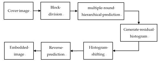
1. Introduction

The data hiding techniques are generally classified into two categories: irreversible data hiding techniques [1,2,3,4,5,6,7] and reversible data hiding techniques [8,9,10,11,12]. In the reversible data hiding technique, secret data can be extracted and the original cover image can be recovered simultaneously. That is why the reversible data hiding techniques are often called the lossless data hiding techniques. Two main approaches for developing reversible data hiding techniques are the difference expansion (DE) [13,14,15,16] and the histogram shifting (HS) [17,18,19,20,21,22,23,24,25,26,27,28,29,30,31,32] approaches. Boato et al. proposed a reversible data hiding scheme that combined the above two approaches in 2012 [15].

In 2006, Ni et al. introduced the concept of the histogram shifting for reversible data hiding [17]. The occurrences of all the possible pixel values in a cover image are calculated to generate the image histogram. Secret data are embedded into the pixels located at the peak points. Basically, the hiding capacity of HS equals the number of the pixels in the peak points used. More pairs of the peak and zero points are required in order to obtain a better hiding capacity while the maximum numbers of the pairs of the peak and zero points are less than or equal to 2 in most of the nature images.

To increase the hiding capacity of HS, several residual histogram shifting (RHS) techniques had been proposed [18,19,20,21,22,23,24]. Different prediction strategies were introduced in these RHS techniques to increase the occurrences of the peak points in the residual image histogram. Among these RHS techniques, the block-based prediction residual histogram shifting (BPRHS) technique proposed by Tsai et al. increases the hiding capacity and resists against the error propagation by using the block-based linear prediction [18]. The reversible data hiding techniques can be improved in order to protect the image integrity. The basic function of the image integrity protection technique is to detect the tamper areas of an image. Lo and Hu extended the BPRHS technique to protect the image integrity for image tamper detection [25]. In addition to detecting the tamper areas, some image integrity protection techniques are capable of roughly recovering the tamper areas.

Those reversible data hiding techniques mentioned above focused on the digital images in raw data format [17,18,19,20,21,22,23,24]. With the increasing demand of privacy protection, the ability to embed information in an encrypted image is desired. In the literature, some reversible data hiding techniques for the encrypted images had been introduced [26,27,28]. Some reversible data hiding techniques for the block truncation coding had been proposed [29,30,31]. An HS-based technique for the compressed images of block truncation coding had been proposed [29]; an RHS-based data hiding scheme had been introduced for the compressed images of the block truncation coding (BTC) [30]. Furthermore, an edge-based quantization approach had been designed for adaptive block truncation coding [31].

To improve the hiding capacity of BPRHS, Hu et al. proposed a cascading prediction approach, which utilizes a two-stage prediction mechanism with a fixed block size of 4 × 4 pixels [32]. In the first stage prediction, a fixed reference pixel is used, and the other pixels are predicted based on the nearest neighbor rule (NNR). To improve the hiding capacity of BPRHS further and to maintain good image quality of the embedded image, this paper proposes an efficient residual histogram shifting technique. The proposed technique extends the previous work [32] by using the multiple-round hierarchical prediction mechanism so that it can work on the images of various block sizes. Furthermore, the reference pixel of a block of n × n pixels where n is even can be selected adaptively to provide more flexibility. One of the four center pixels in each block can be selected to act as the reference pixel. According to the results, the hiding capacity and the embedded image quality are approximately the same when different reference pixels are used. The selection of reference pixel can provide additional security protection for data embedding. This paper is organized as follows. The review of the BPRHS technique is given in Section 2. Section 3 presents the proposed technique. Experimentation is conducted in Section 4. Finally, Section 5 concludes this paper.

2. Review on the BPRHS Technique

The BPRHS technique was proposed to increase the hiding capacity of the HS scheme [18]. In the HS scheme, the image histogram is generated and used to embed the secret data. The hiding capacity of HS is limited by the occurrences of pixels located at the peak points of the image histogram. To improve the hiding capacity of HS, the residual image histogram of the prediction errors will be generated and used to hide the secret data in BPRHS.

First, the cover image is partitioned into non-overlapped image blocks of n × n pixels. The center pixel in each block is selected as the reference pixel for block-based prediction. Except for the reference pixel, there are n × n−1 pixels in each n × n block. The prediction error (pe) of each remaining pixel can be computed by Equation (1):

$$pe=rdp-refp.$$

(1)

where, rdp and refp denote the remaining pixel and the reference pixel, respectively.

By sequentially executing the block-based prediction process of each image block, all the prediction errors are computed to generate the residual image histogram. Let pno denote the number of pairs for peak and zero points used for secret data embedding. These pno pairs of peak and zero points are searched from the residual image histogram. Then, secret data is embedded into the prediction errors located at the peak points, and the prediction errors between the peak and zero points are shifted accordingly. Finally, the reverse block-based prediction process is executed to generate the embedded image.

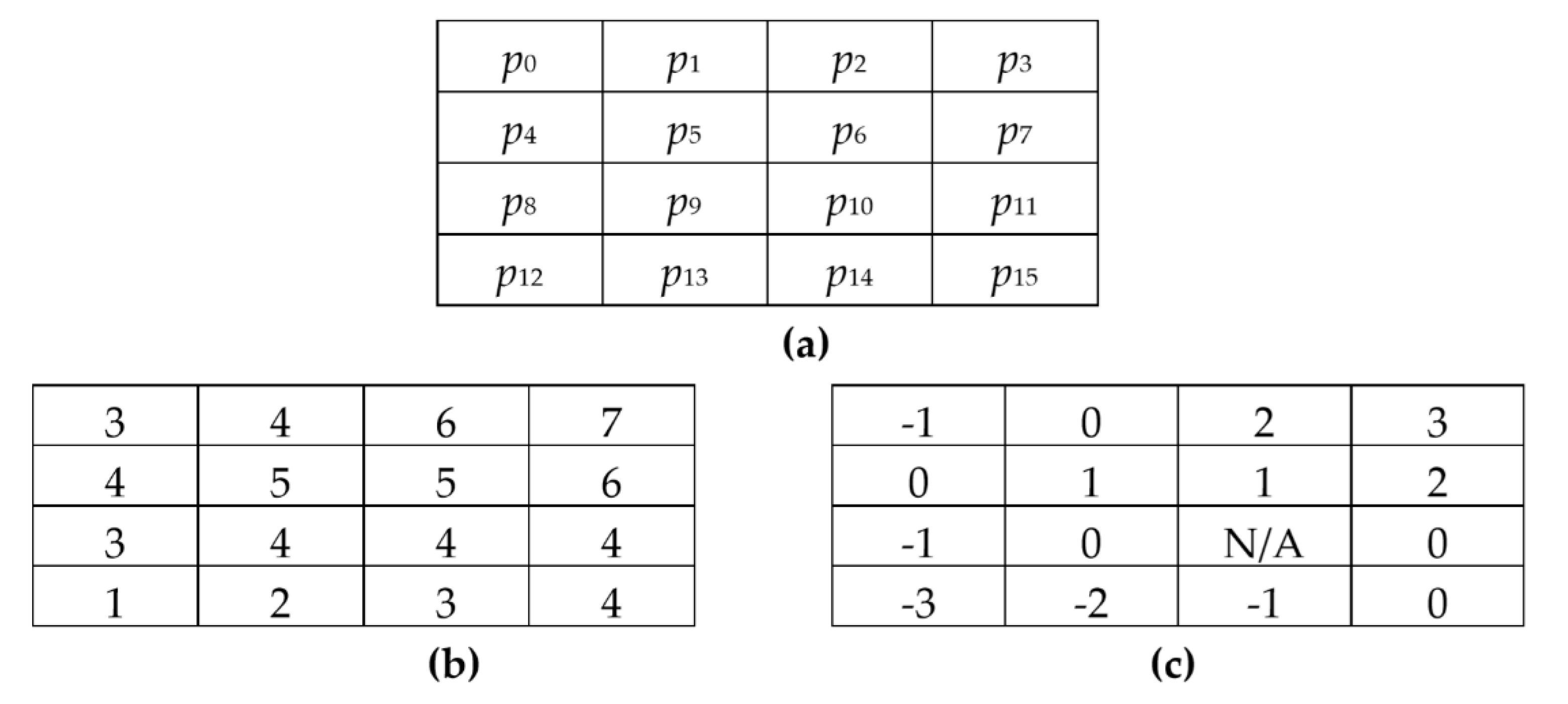
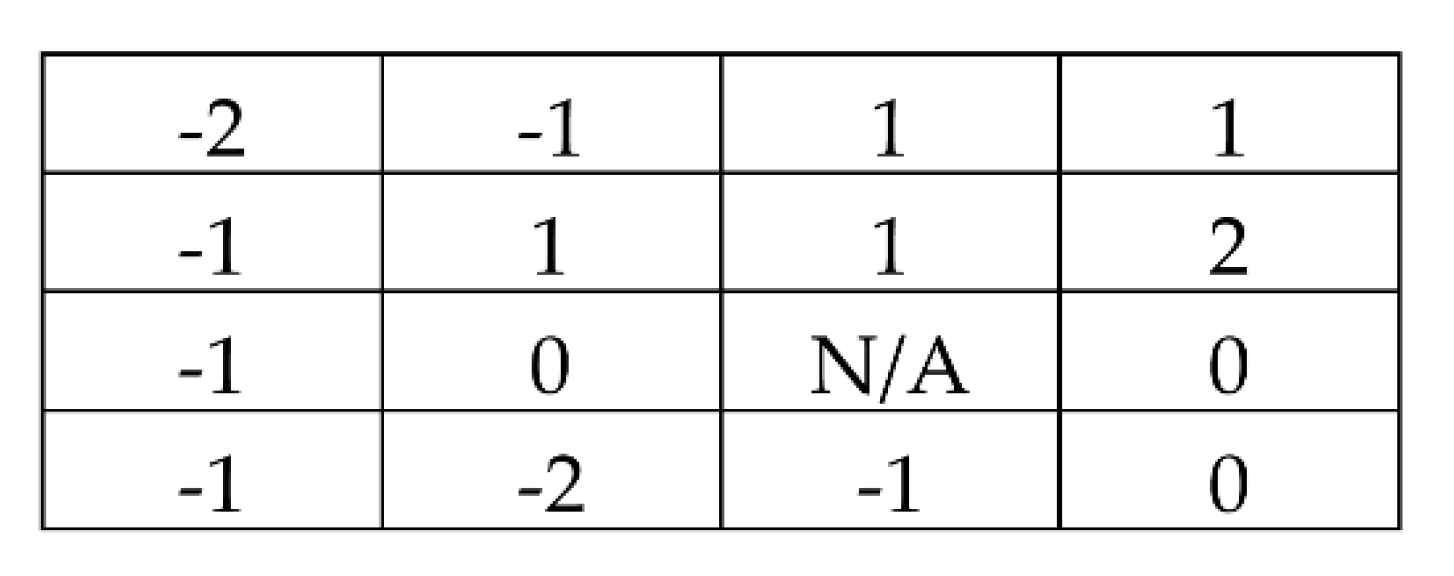
An example of block-based prediction for the 4 × 4 image block by using BPRHS with pno = 2 is described as below. The position diagram of the pixels is given in Figure 1a. In BPRHS, p₁₀ is taken as the reference pixel. The test image block of 4 × 4 pixels is listed in Figure 1b. A total of 15 prediction errors of the test block using BPRHS are shown in Figure 1c. 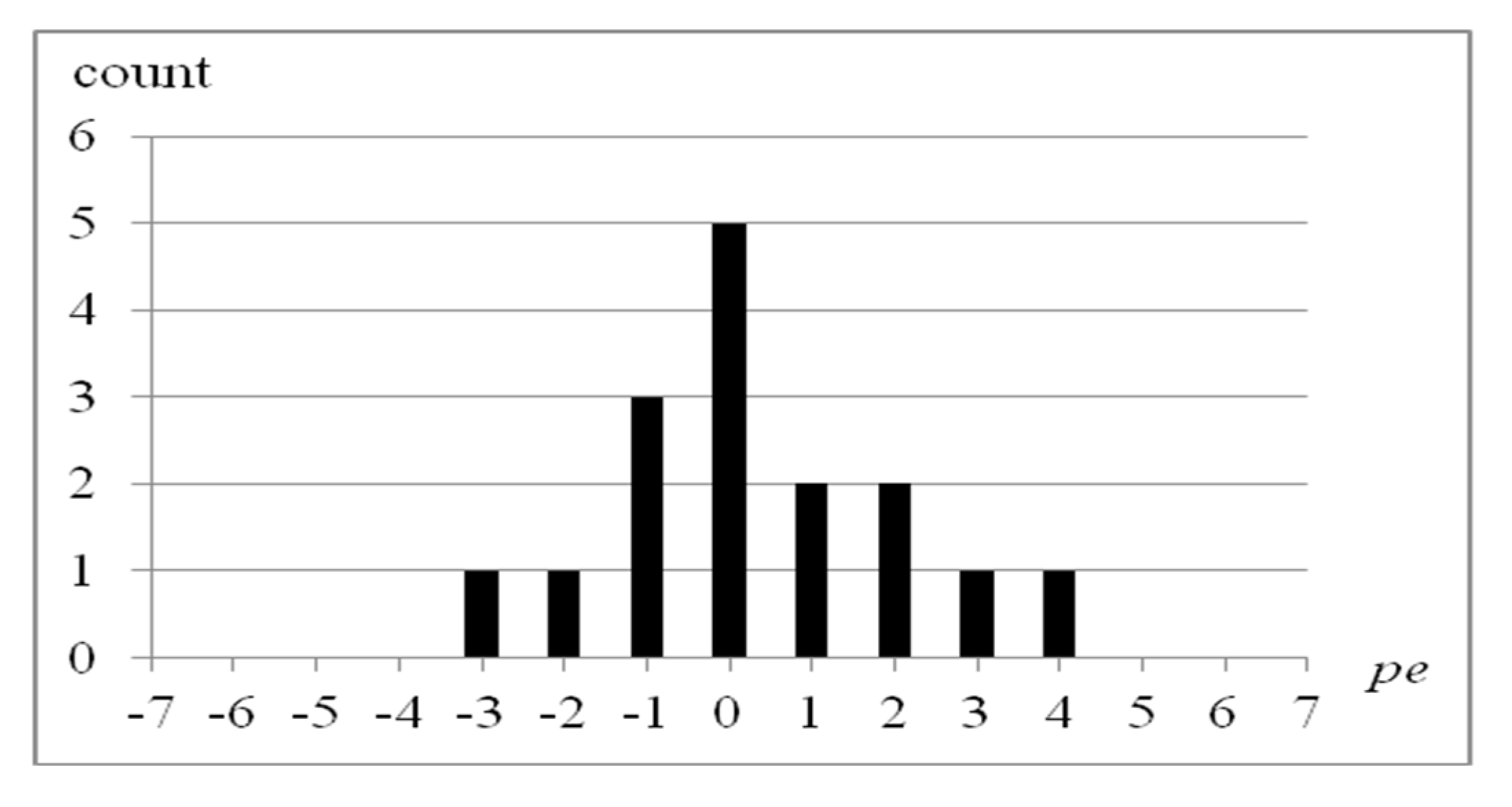Since there is no prediction error for the center pixel p₁₀, the corresponding prediction error of p₁₀ is marked as not available (N/A). The resultant residual image histogram of BPRHS is shown in Figure 2. Two pairs of peak and zero points (0,−4) and (2,5) are searched from this residual image histogram. These two pairs of peak and zero points are used in the residual histogram shifting process to embed the secret data. The hiding capacity of the BPRHS is 7 bits when the pno value is set to 2.

3. Proposed Technique

The goal of the proposed technique is to extend the hiding capacity of the BPRHS scheme when the block size is greater than 4 × 4. The proposed technique extends Hu’s scheme [32] by using the multiple-round hierarchical prediction mechanism. In Hu’s scheme, a two-stage prediction mechanism with a fixed block size of 4 × 4 pixels was introduced. In the first stage prediction, a fixed reference pixel is used, and the other pixels are predicted based on the nearest neighbor rule (NNR). It is obvious that the reference pixel usually has a lower degree of similarity to the pixels which are far away from it when the block size increases. To increase the occurrences of the peak points in the residual image histogram, the hierarchical prediction mechanism is designed in the proposed technique. Two prediction models are designed in the multiple-round prediction mechanism.

3.1. Data Embedding

In the proposed technique, the cover image is partitioned into non-overlapping image blocks of n × n pixels. Let pno denote the number of pairs of peak and zero points used for secrete data embedding. The value of pno is usually determined according to user’s requirement or the size of the embedded secret data. The multiple-round prediction mechanism is employed to sequentially process the image blocks in the order of left-to-right and top-to-bottom. For each block to be processed, the number of rounds (rno) that will be used in the hierarchical prediction mechanism should be determined first. The number of rounds needed for an n × n image block can be computed by Equation (2):

$$rno=\lceil \frac{n-1}{2}\rceil .$$

(2)

In case of the block size of 3 × 3, only one round of prediction is needed; two rounds are required for the block sizes of 4 × 4 and 5 × 5; three rounds are required in case of the block sizes of 6 × 6 and 7 × 7.

For each n × n block to be processed, the reference pixel in each block is to be determined. The value of n may be either odd or even so two possible cases can be found in determining the reference pixel of each block. First, the center pixel in the image block is taken as the reference pixel when n is odd. The same rule cannot be employed when n is even because four center pixels are found in each block. Only one of these four candidates can be selected as the reference pixel in the proposed technique. Recall that a fixed center pixel is selected as the reference pixel in BPRHS. In the proposed technique, the reference pixel can be adaptively selected by the user.

The index/indices idx of the center pixel for an n × n image block can be computed by Equation (3):

$$idx=\{\begin{array}{ll}\lfloor \frac{n\times n}{2}\rfloor \hfill & \hfill \mathrm{if}n\mathrm{is}\mathrm{odd}\\ \frac{n}{2}(n+1)-n-1,\frac{n}{2}(n+1)-n,\frac{n}{2}(n+1)-1,\frac{n}{2}(n+1)\hfill & \hfill \mathrm{if}n\mathrm{is}\mathrm{even}\end{array}.$$

(3)

According to the above Equation, the index of the center pixel equals 12 when the block size is 5 × 5. The indices of the center pixels are 5, 6, 9, and 10 when the block size is set to 4 × 4. Among these four center pixels, one will be selected as the reference pixel in the prediction process.

This study proposes two models of error prediction. The first round of the prediction process is the same for both of the two prediction models. Once the reference pixel is determined, the first round is executed. The prediction error (pe) of each directly adjacent pixel (dap) to the reference pixel (rp) is computed according to Equation (4):

$$pe=dap-rp.$$

(4)

where dap and rp denote the directly adjacent pixel and the reference pixel, respectively.

Let crno denote the current round number for block-based prediction. Initially, crno is set to 1. The first round of prediction mentioned above is first executed. Only 8 directly adjacent pixels of the reference pixel are processed. If rno is greater than 1, the succeeding rounds of the prediction process are executed. Otherwise, the prediction process stops.

In each succeeding round of the prediction, crno is increased by 1. The remaining pixels adjacent to the pixels processed in the previous round are selected. The closest adjacent pixel of each selected pixel is taken as the reference pixel. Here, the reference pixel is adaptively determined for each selected pixel based on NNR. The prediction error of each selected pixel (sp) to its nearest neighboring pixel (nnp) can be computed according to Equation (5):

$$pe=sp-nnp.$$

(5)

If crno is less than rno, the above process can be extended round by round until all the pixels in this block are processed.

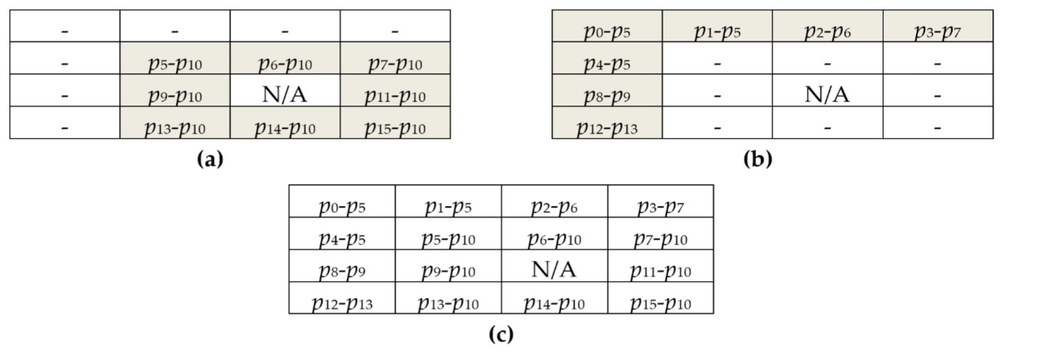
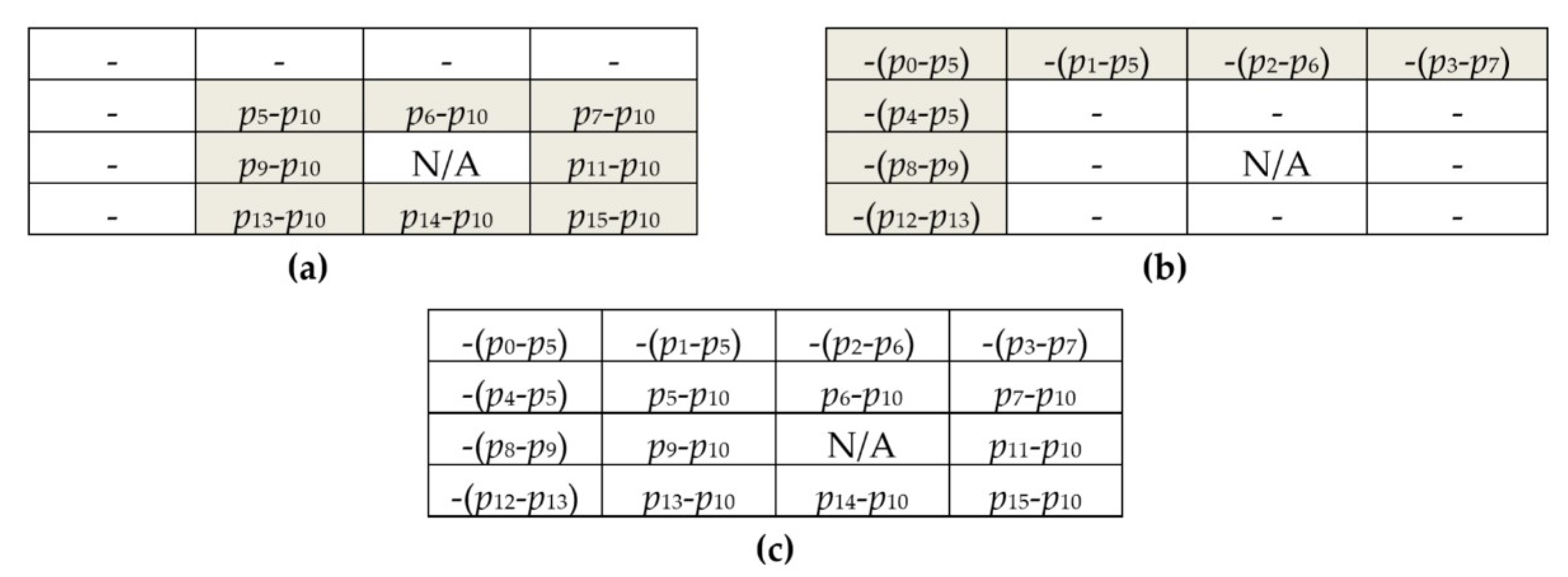
The above process is also called the first prediction model. Figure 3 depicts the first prediction model for 4 × 4 blocks. Here, the center pixel p₁₀ is taken as the reference pixel of the image block. In the first round of prediction, eight prediction errors shown in Figure 3a of these directly adjacent pixels to the center pixel are computed. In the second round of the prediction process, the remaining seven prediction errors are computed as shown in Figure 3b. Here, p₅ is taken as the reference pixel for p₀, p₁, and p₄. Besides, p₆, p₇, p₉, and p₁₃ are taken as the reference pixels for p₂, p₃, p₈, and p₁₂, respectively. The prediction errors of this block are shown in Figure 3c.

Taking the test image block in Figure 1b as an example, the prediction errors of this block by the proposed multiple-round prediction mechanism are shown in Figure 4. A total of 15 prediction errors are generated by the proposed prediction mechanism for this 4 × 4 image block. The resultant residual image histogram of the prediction errors is shown in Figure 5.

Following this example, two pairs of peak and zero points are searched by this residual image histogram. They are (−1,−3) and (1,3). The maximal value of pno equals 2 in this example. The hiding capacities of the proposed technique are 5 and 9 bits when pno values are set to 1 and 2, respectively.

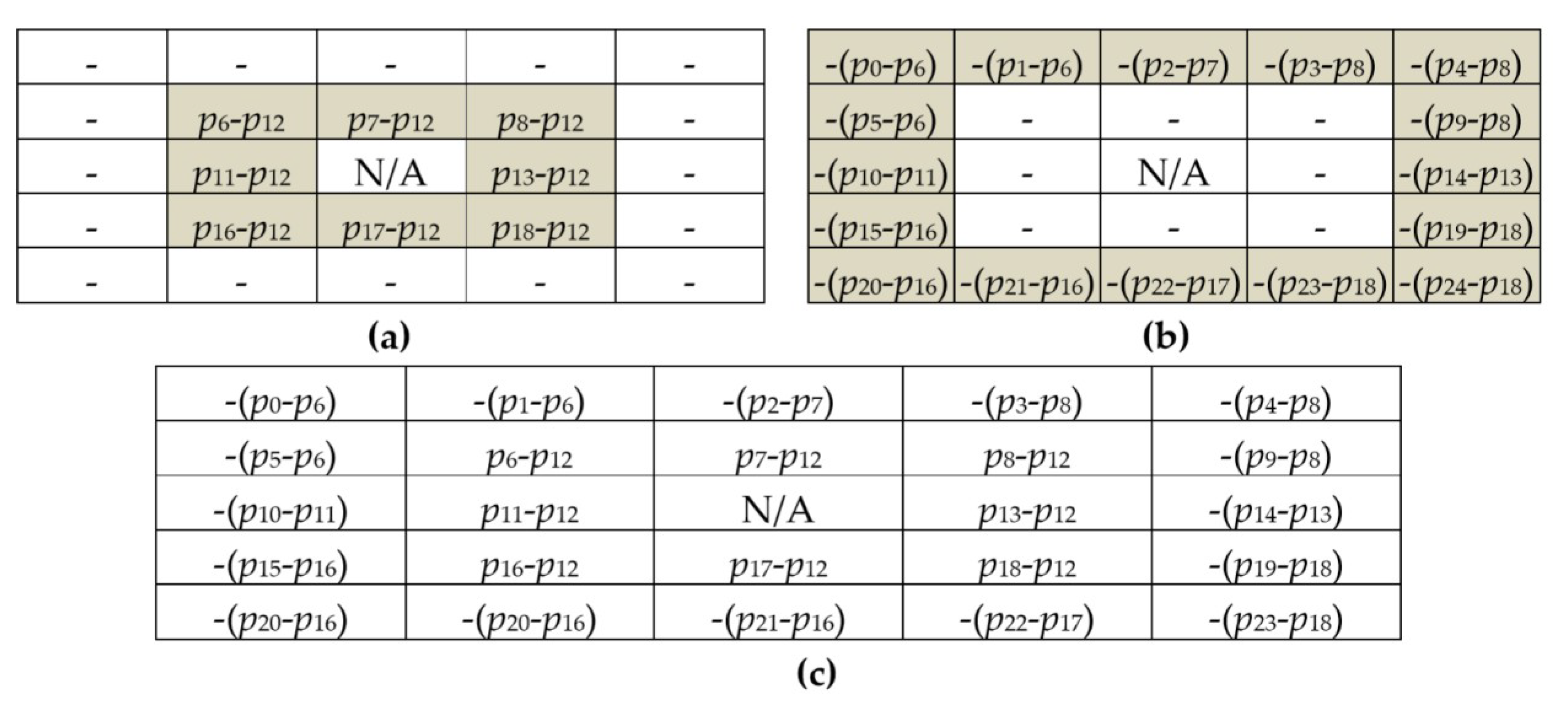
In addition to the first prediction model, we design the second prediction model based on the first one. The first round of the prediction process for the second prediction model is the same as that of the first prediction one. The prediction error of each directly adjacent pixel to the reference pixel can be computed according to Equation (3).

If there exist some remaining pixels to be processed in the succeeding rounds, the prediction error of each selected pixel (sp) to its nearest neighboring pixel (nnp) is computed according to Equation (6):

$$pe={\left(-1\right)}^{(crno+1)}\times \left(sp-nnp\right).$$

(6)

Figure 6 depicts the second prediction model for the 4 × 4 block. Similarly, the center pixel p₁₀ is taken as the reference pixel of the image block. In the first round of the prediction process, eight prediction errors shown in Figure 6a of these directly adjacent pixels to the center pixel are computed. In the second round of the prediction process, the remaining seven prediction errors are computed as shown in Figure 6b. The prediction errors of this block are shown in Figure 6c.

In Figure 7 and Figure 8, the two prediction models for the 5 × 5 image block are depicted, respectively. Two rounds of the prediction process are performed to generate the prediction errors for the pixels in the image block of 5 × 5 pixels. A total of 24 prediction errors are generated after the multiple-round prediction mechanism is executed. In fact, the proposed hierarchical prediction mechanism can be extended for the image blocks of n × n pixels where n is greater than 5.

When the prediction errors of each n × n image block are computed by using the multiple-round prediction mechanism, the occurrences of all the possible residual values are calculated to generate the residual image histogram. After the residual image histogram is constructed, pno pairs of peak and zero points are then searched from the residual image histogram. The hiding capacity of the image equals the sum of the occurrences of the residual values located at these peak points.

Secret data are then embedded into the residual values in the peak points and the prediction errors between the peak and zero points will be shifted accordingly. After the secret data are embedded into the residual values, the embedded image can be generated by performing the reverse multiple-round prediction mechanism.

3.2. Data Extraction

The goal of the data extraction procedure is to extract secret data from the embedded image. In addition, the original cover image will be recovered after the secret data is extracted. Before the data extraction procedure is performed, the values of some system parameters, such as W, H, n, pno, the pairs of peak and zero points, and the prediction model used should be available.

First, the selected linear prediction model used in the data embedding procedure is applied on the embedded image to generate the residual embedded-image. The prediction errors of the residual embedded-image are examined to extract the embedded secret data and to recover the original cover image.

To extract the secret data, the prediction errors in each n × n block is sequentially processed in the raster scanning order. If the prediction error pe is not within any pair of the peak and zero points, pe is kept unchanged. Otherwise, three cases are discussed for pe that is within one specific pair of peak point and zero point. In the first case, if pe is located at the peak point, 1-bit secret data valued at 1 is extracted and the value of pe is unchanged. In the second case, if the zero point is smaller than the peak point and pe is smaller than the peak point by 1, 1-bit secret data value 0 is extracted and the value of pe is replaced by the value of the peak point. If the zero point is greater than the peak point and pe is greater than the peak point by 1, 1-bit secret data value 0 is extracted and the value of pe is replaced by the value of the peak point. Lastly, the remaining prediction errors are shifted close to peak point by 1 and no secret data is extracted. By sequentially processing the residual blocks in the rater scanning order, the embedded secret data is extracted from the residual embedded-image. Meanwhile, the original cover image is recovered by performing reverse linear prediction of the selected prediction model on the reconstructed embedded-image.

4. Results

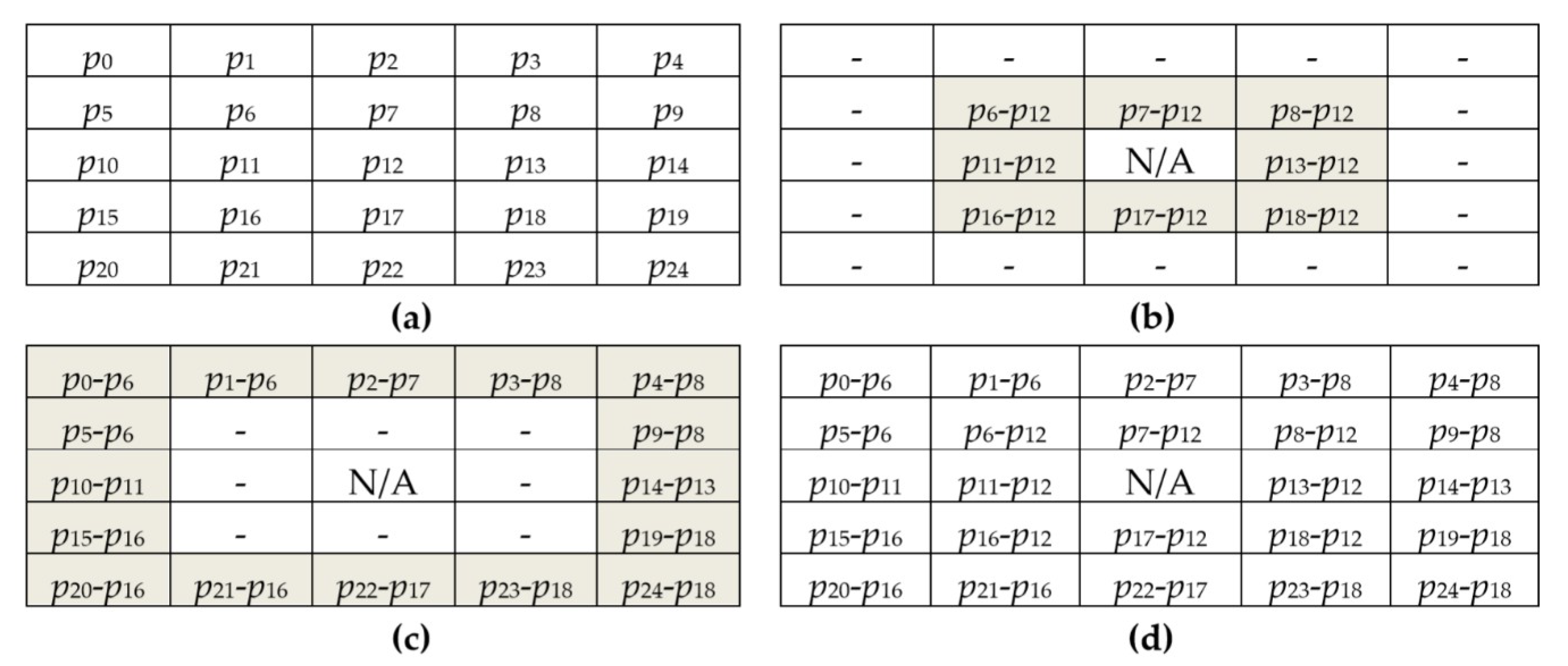
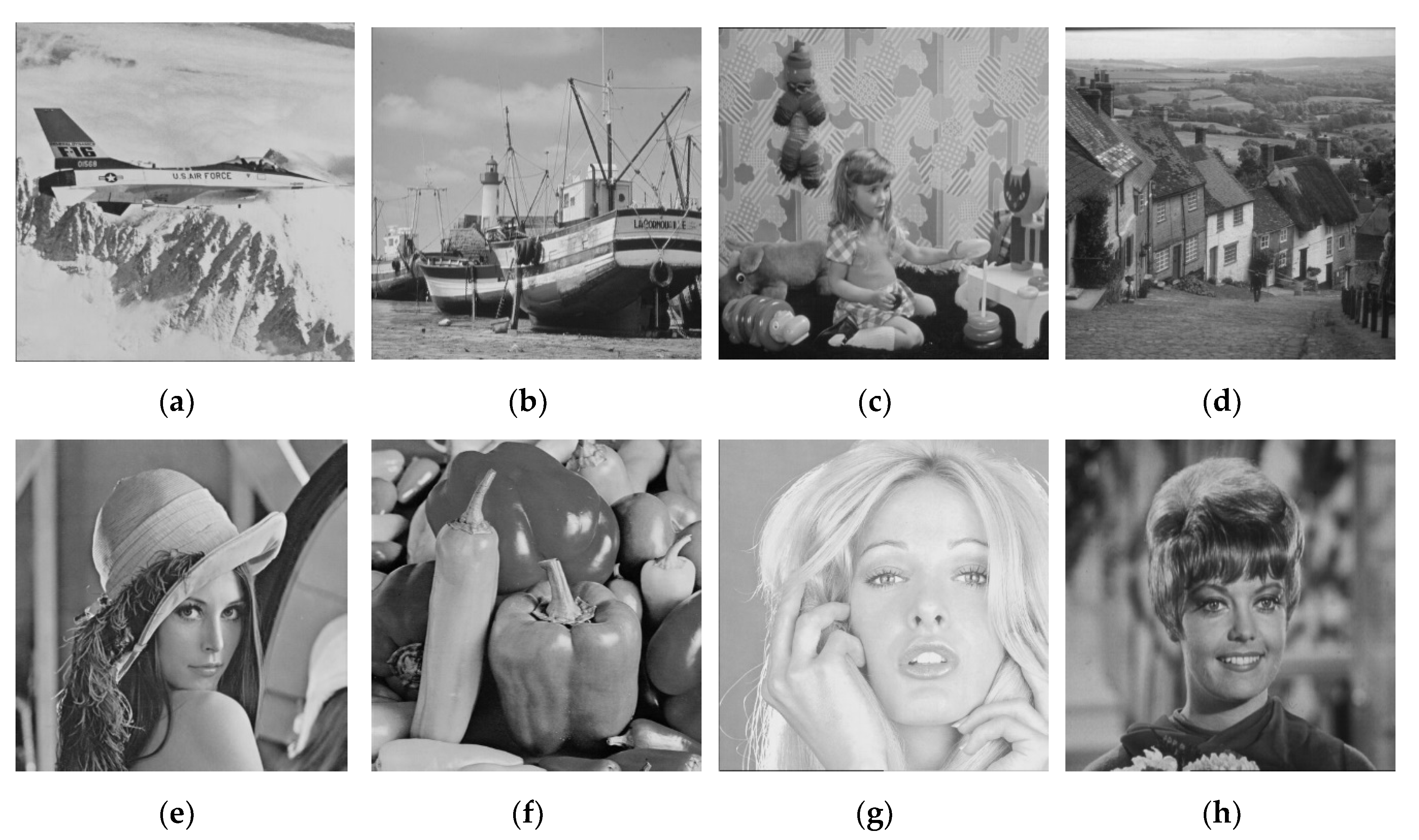
Our experiments are performed on a Window 10 computer with Intel Core i7 3.6 GHz CPU and 16 GB random access memory (RAM). The testing programs are implemented in Bloodshed Dev C++. In our experiments, eight grayscale images of 512 × 512 pixels, “Airplane”, “Boat’, “Girl”, “Goldhill”, “Lenna”, “Pepper”, “Tiffany”, and “Zelda” in Figure 9, are used. These testing images are downloaded from the USC SIPI image database.

To measure the image quality of the embedded image, the mean square error (MSE) among the cover image and the embedded image of W × H pixels is defined as Equation (7):

$$MSE=\frac{1}{W\times H}{\displaystyle \sum _{i=1}^W{\displaystyle \sum _j^H{(o_{ij}-r_{ij})}^{{}_2}}}.$$

(7)

where o_ij and e_ij denote the grayscale pixels in the cover image and the embedded image, respectively.

Besides, the peak signal-to-noise ratio (PSNR) between the cover image and the embedded image is calculated by Equation (8):

$$PSNR=10\times {\log }_{10}\frac{{255}^2}{MSE}dB.$$

(8)

Generally, PSNR is considered as an indication of image quality rather than a definitive computation. It is a common measure for evaluating image quality. A large PSNR value indicates that the difference between two given images is quite small.

The results of the hiding capacity of the proposed technique with the two prediction models when the block size is 4 × 4 are listed in

Table 1. Results of the hiding capacity of the proposed technique with the first prediction model when the block size is set to 4 × 4.

Images	refp = p5		refp = p6		refp = p9		refp = p10
	pno = 1	pno = 2	pno = 1	pno = 2	pno = 1	pno = 2	pno = 1	pno = 2
Airplane	417,43	714,42	415,82	714,75	416,63	714,89	413,28	714,06
Boat	249,73	481,52	250,43	482,17	250,91	481,55	249,38	481,16
Girl	269,04	514,76	266,62	512,04	267,43	519,98	262,55	514,21
Goldhill	199,25	385,54	199,81	385,72	198,73	383,58	199,05	385,01
Lenna	288,48	537,21	287,58	539,25	286,58	537,72	287,85	537,76
Pepper	173,41	330,12	172,53	330,29	173,99	330,53	171,37	329,50
Tiffany	321,22	574,53	316,34	574,41	319,57	576,30	320,74	574,19
Zelda	277,21	539,25	278,16	540,61	277,52	535,75	276,90	540,22
Average	274,47.1	509,66.9	273,41.1	509,90.5	273,92.0	510,03.8	272,64.0	509,51.4

and

Table 2. Results of the hiding capacity of the proposed technique with the second prediction model when the block size is set to 4 × 4.

Images	refp = p5		refp = p6		refp = p9		refp = p10
	pno = 1	pno = 2	pno = 1	pno = 2	pno = 1	pno = 2	pno = 1	pno = 2
Airplane	417,43	715,60	415,82	715,14	416,63	716,63	413,28	711,34
Boat	249,73	482,20	250,43	483,66	250,91	482,87	249,38	480,78
Girl	269,04	523,45	266,62	511,94	267,43	514,62	262,55	517,88
Goldhill	199,25	387,51	199,81	383,80	198,73	382,63	199,05	386,47
Lenna	288,48	534,93	287,58	538,42	286,58	536,23	287,85	535,72
Pepper	173,41	331,18	172,53	331,21	173,99	332,83	171,37	330,76
Tiffany	321,22	576,98	316,34	573,83	319,57	574,90	320,74	577,04
Zelda	277,21	540,57	278,16	537,45	277,52	535,91	276,90	540,48
Average	274,47.1	511,55.3	273,41.1	509,43.1	273,92.0	509,57.8	272,64.0	510,05.9

, respectively. In the simulations, one of these four center pixels is selected as the reference pixel (refp). The same hiding capacities are obtained in these two prediction models when pno is set to 1. The average hiding capacities of 274,47.125, 273,41.125, 273,92, and 272,64 bits are achieved with pno is set to 1 when the reference pixels are p₅, p₆, p₉, and p₁₀, respectively.

The second prediction model performs slightly better hiding capacity than the first one when pno is set to 2. The average hiding capacities of 511,55.25, 509,43.13, 509,57.75, and 510,05.875 bits are achieved when pno to 2 in the second prediction model, and the reference pixels are p₅, p₆, p₉, and p₁₀, respectively. The results indicate the best hiding capacity is achieved in the proposed technique when the reference pixel is p₅.

Table 3. Results of the image quality of the proposed technique with the first prediction model when the block size is set to 4 × 4.

Images	refp = p5		refp = p6		refp = p9		refp = p10
	pno = 1	pno = 2	pno = 1	pno = 2	pno = 1	pno = 2	pno = 1	pno = 2
Airplane	49.542	48.088	49.497	48.069	49.547	48.083	49.540	48.063
Boat	49.282	48.002	49.308	47.976	49.314	48.005	49.275	47.975
Girl	49.050	47.276	48.949	47.283	49.466	47.325	49.402	47.373
Goldhill	49.031	47.325	49.059	47.330	49.018	47.303	49.013	47.315
Lenna	49.219	47.497	49.283	47.577	49.291	47.557	49.238	47.551
Pepper	49.119	47.661	49.050	47.652	49.159	47.662	49.058	47.645
Tiffany	49.472	48.213	49.472	48.173	49.473	48.195	49.466	48.199
Zelda	49.126	47.435	49.116	47.458	49.119	47.453	49.148	47.462
Average	49.230	47.687	49.217	47.690	49.298	47.698	49.268	47.698

and

Table 4. Results of the image quality of the proposed technique with the second prediction model when the block size is set to 4 × 4.

Images	refp = p5		refp = p6		refp = p9		refp = p10
	pno = 1	pno = 2	pno = 1	pno = 2	pno = 1	pno = 2	pno = 1	pno = 2
Airplane	51.929	48.251	51.922	48.244	51.961	48.210	51.970	48.167
Boat	51.985	48.104	52.009	48.060	52.017	48.103	51.954	48.072
Girl	51.719	47.347	51.526	47.378	51.383	47.310	51.589	47.323
Goldhill	51.566	47.362	51.539	47.360	51.540	47.333	51.563	47.339
Lenna	51.573	47.555	51.590	47.646	51.585	47.598	51.605	47.632
Pepper	51.806	47.705	51.823	47.692	51.861	47.706	51.811	47.689
Tiffany	52.043	48.337	52.029	48.243	52.010	48.290	52.070	48.290
Zelda	51.521	47.514	51.524	47.526	51.527	47.527	51.513	47.525
Average	51.768	47.772	51.745	47.769	51.736	47.760	51.759	47.755

list the results of the image quality of the first and second prediction models of the proposed technique when the block size is set to 4 × 4, respectively. Compared to the first prediction model, the second prediction model provides much better image quality when pno is set to 1. According to the results in Table 3, average PSNR values of 49.230, 49.217, 49.298, and 49.268 dB are achieved by using the first prediction model when pno is set to 1, and the reference pixels are p₅, p₆, p₉, and p₁₀, respectively. Compared to the first prediction model, average image quality gains of 2.291 dB, 2.307 dB, 2.229 dB, and 2.245 dB are achieved by using the second prediction model when pno is set to 1, and the reference pixels are p₅, p₆, p₉, and p₁₀, respectively.

Compared to the first prediction model, slightly worse PSNR values are obtained using the second prediction model when pno is set to 2. Average PSNR values of 47.772 dB, 47.769 dB, 47.760 dB, and 47.755 dB are achieved by using the first prediction model when pno is set to 2, and the reference pixels are p₅, p₆, p₉, and p₁₀, respectively. According to the results in Table 3 to Table 4, it is shown that the best image quality is achieved in the proposed technique when the reference pixel is set to p₅.

Results of these two prediction models proposed in this paper when the block size is set to 5 × 5 are listed in

Table 5. Results of the hiding capacity and embedded image quality of the proposed technique with the first prediction model when the block size is set to 5 × 5.

Images	Hiding Capacity			Embedded Image Quality
	pno = 1	pno = 2	pno = 3	pno = 1	pno = 2	pno = 3
Airplane	414,39	718,03	718,05	48.615	47.371	47.371
Boat	253,92	491,23	491,26	48.450	47.446	47.445
Girl	266,34	506,63	506,78	48.149	46.565	46.565
Goldhill	202,69	387,74	387,79	48.115	46.626	46.625
Lenna	286,74	539,39	539,46	48.239	46.790	46.790
Pepper	269,43	512,75	512,79	48.294	42.650	42.650
Tiffany	320,34	580,28	580,44	48.555	47.598	47.598
Zelda	282,22	546,78	546,85	48.166	46.689	46.689
Average	287,00.9	535,35.4	535,42.8	48.323	46.467	46.467

and

Table 6. Results of the hiding capacity and embedded image quality of the proposed technique with the second prediction model when the block size is set to 5 × 5.

Images	Hiding Capacity			Embedded Image Quality
	pno = 1	pno = 2	pno = 3	pno = 1	pno = 2	pno = 3
Airplane	414,39	718,81	718,85	51.784	47.529	47.528
Boat	253,92	489,62	489,65	51.930	47.542	47.542
Girl	266,34	506,27	506,42	51.212	46.653	46.653
Goldhill	202,69	388,02	388,05	51.362	46.680	46.680
Lenna	286,74	540,19	540,26	51.371	46.911	46.911
Pepper	269,43	511,46	511,50	51.518	42.387	42.387
Tiffany	320,34	580,83	580,86	51.964	47.700	47.700
Zelda	282,22	547,71	547,80	51.260	46.784	46.783
Average	287,00.9	535,36.4	535,42.4	51.550	46.523	46.523

, respectively. These two prediction models provide similar hiding capacities. Average hiding capacities of 287,00.875, 535,35.375, and 535,42.75 bits are achieved by the first prediction model when the pno values are 1, 2, and 3, respectively.

Compared to the first prediction model, the second prediction model provides much higher PSNR values. Average PSNR values of 51.550 dB, 46.523 dB, and 46.523 dB are achieved by the second prediction model when the pno values are 1, 2, and 3, respectively. Compared to the result by first prediction model, average image quality gains of 3.227 dB, 0.056 dB, 0.056 dB are achieved by the second prediction model when the pno values are 1, 2, and 3, respectively.

The comparative techniques and the proposed technique are analyzed and shown in

Table 7. Average results of the hiding capacity and embedded image quality of the comparative techniques.

Images	Hiding Capacity		Embedded Image Quality
	pno = 1	pno = 2	pno = 1	pno = 2
HS	431,7.000	837,7.125	53.094	48.264
BPRHS-4 × 4	245,27.625	464,55.375	51.939	49.320
BPRHS-5 × 5	230,76.375	436,70.250	51.764	49.148
CM	284,66.625	531,80.125	49.184	47.240
PT1-4 × 4	274,47.125	509,66.875	49.230	47.687
PT1-5 × 5	287,00.875	535,35.375	48.323	46.467
PT2-4 × 4	274,47.125	511,55.250	51.768	47.772
PT2-5 × 5	287,00.875	535,36.375	51.550	46.523

. The average results of these techniques examined by eight test images are listed. HS and CM represent the histogram shifting technique [17] and the comparative method [32], respectively. BPRHS-4 × 4 and BPRHS-5 × 5 stand for the BPRHS with the block sizes of 4 × 4 and 5 × 5, respectively. PT1-4 × 4 and PT1-5 × 5 denote the proposed technique with the first prediction model when the block sizes are 4 × 4 and 5 × 5, respectively. PT2-4 × 4 and PT2-5 × 5 denote the proposed technique with the second prediction model when the block sizes are 4 × 4 and 5 × 5, respectively. It is shown that the hiding capacities of BPRHS-5 × 5 is less than those of BPRHS-4 × 4. This is because a fixed reference pixel in each block is used by BPRHS. The prediction error becomes inaccurate when the processed pixel is far away from the reference pixel.

However, this problem is not found in the proposed technique. According to the results reported in Table 3, Table 4, Table 5 and Table 6, it is shown that the hiding capacity of the proposed technique increases with the increments of the block size. This result indicates that the proposed multiple-round prediction mechanism indeed solves the problem that may occur when using BPRHS. Among these schemes, PS2-5 × 5 outperforms these comparative schemes.

According to the results, the proposed technique provides a better hiding capacity than HS and BPRHS. Compared to the results by HS and BPRHS, average hiding capacity gains of 427,78.125 and 4699.875 bits are achieved by the proposed technique when pno is set to 2, and the block size is set to 4 × 4, respectively. Good image quality of the embedded images is achieved by the proposed technique. From the results, average PSNR values of 51.768 dB and 47.772 dB are achieved by the proposed technique when the block size of 4 × 4, and the values of pno are set to 1 and 2, respectively.

In the data hiding techniques based on the histogram shifting technique, the value of pno and the pairs of peak and zero points should be stored additionally. If the overflow/underflow problem occurs, additional information is recorded so that the reversible property can be preserved. In the simulations demonstrated for comparative studies in this section, no overflow/underflow problem is encountered. That is due to the fact that the max number of pairs is set to 3.

A major problem of BPRHS is that the hiding capacity decreases with the increase of the block size. That is because a fixed reference pixel is used to generate the prediction for all the other pixels in BPRHS. This problem is solved by the multiple-round prediction mechanism in the proposed technique. The reference pixel is adaptively determined for each selected pixel based on the NNR in the multiple-round prediction mechanism. From the results, it is obvious that the use of the multiple-round prediction in the proposed technique compared to BPRHS achieves higher occurrences of the peak points in the residual histogram. Moreover, good visual quality of the embedded image is achieved by the proposed technique, as demonstrated from the experimental results.

5. Conclusions

An efficient residual histogram shifting technique based on the block-based prediction histogram shifting technique had been proposed in this paper. The multiple-round prediction mechanism was designed in this paper to generate the prediction errors for each image block. Two prediction models were employed in the prediction mechanism. Experimental results verify that the proposed technique outperforms the comparative methods in terms of the hiding capacity. Meanwhile, good image quality of the embedded image is obtained in the proposed technique.

The proposed technique generates the prediction errors in the block-by-block manner in the same way as BPRHS [18] and the comparative method [32]. Therefore, these three schemes have the error-propagation-free property. The grayscale image integrity protection scheme based on BPRHS had been proposed [25] for image tamper detection. Since the hiding capacity of the proposed technique is higher than that of BPRHS, we will exploit the possibility to extend the proposed technique for grayscale image tamper detection in the future.