Article

A Bidirectional Searching Strategy to Improve Data Quality Based on K-Nearest Neighbor Approach

1
School of Mechanical and Automotive Engineering, Shanghai University of Engineering Science, Shanghai 201620, China
2
Business School, University of Shanghai for Science and Technology, Shanghai 200093, China
*
Author to whom correspondence should be addressed.
Symmetry 2019, 11(6), 815; https://doi.org/10.3390/sym11060815
Submission received: 16 April 2019 / Revised: 6 June 2019 / Accepted: 18 June 2019 / Published: 20 June 2019

Abstract

:
Traffic data are the basis of traffic control, planning, management, and other implementations. Incomplete traffic data that are not conducive to all aspects of transport research and related activities can have adverse effects such as traffic status identification error and poor control performance. For intelligent transportation systems, the data recovery strategy has become increasingly important since the application of the traffic system relies on the traffic data quality. In this study, a bidirectional k-nearest neighbor searching strategy was constructed for effectively detecting and recovering abnormal data considering the symmetric time network and the correlation of the traffic data in time dimension. Moreover, the state vector of the proposed bidirectional searching strategy was designed based the bidirectional retrieval for enhancing the accuracy. In addition, the proposed bidirectional searching strategy shows significantly more accuracy compared to those of the previous methods.

1. Introduction

For intelligent transportation systems (ITS), traffic data is important for successfully maintaining the utility of the each module [1,2,3]. Traffic data can reflect traffic conditions, but in different manners and provide various information for traffic management, planning, and decision-making [4]. In additional, a series of efficient and flexible solution can be constituted based on the various traffic data for enhancing the travel convenience and mitigating travel costs [5,6,7]. However, due to mechanical faults and changes in the system behavior, the collected traffic data often have corrupted or missing data points, bringing some error to analysis result [8,9]. The quality of traffic data not only deeply affects the analysis results of traffic flow operation, but also affects the efficiency of the traffic system operation [10,11,12]. For these reasons, increasingly more methods have been developed to measure and improve the traffic data quality in the past.
Data recovery aims to improve data quality and enhance the availability of the database. Generally speaking, abnormal data are widespread in the history database [13]. Managing missing data is a common challenge in all areas of science [14]. Sensor failure, transmission network failures, and environmental factors often lead to generate various data quality problems (incompleteness, error, noise, etc.) [15,16]. In order to detect and recover the abnormal data while improving the data quality, in this paper, a novel bidirectional searching strategy was developed based on the k-nearest neighbor (KNN) approach. Note that the bidirectional retrieval strategy involves a symmetric state vector aiming to improve traffic quality considering the correlation of traffic data in time dimension.
The rest of this paper is organized as follows. In the next section, the existing literature in the area of improving data quality will be reviewed. In Section 3, data analysis, abnormal data detected, and model parameter selection can be shown. In Section 4, basic KNN approach will be introduced. In Section 5, a novel bidirectional data recovery approach is proposed, and the parameter setting process is presented. Section 6 discusses the experimental design and the results. Section 7 concludes the paper with a summary of bidirectional searching strategy and gives the suggestions for future work.

2. Literature Review

Several works focusing on recovering the abnormal data response to the data quality control strategy. These studies examine the effect of abnormal data and research the data recovery approach based on the historical aiming to improve data quality. Pushkar et al. [17] applied the catastrophe theory to establish the three-parameter sudden change surface of traffic flow to recover data and then proposed the speed estimation method. A nearest-neighbor imputation algorithm was developed and applied to interpolate the missing data based on the average value of historical data at the same time interval [18]. In addition, the factor approach estimated the missing data by using the mean value of the key factors selected from the historical set [19]. Troyanskaya et al. [20] investigated automated methods for estimating missing data to minimize the effect of incomplete data sets on analyses. Smith et al. [21] performed a preliminary analysis of several heuristic and statistical imputation techniques and declared the statistical techniques are more accurate. Chen et al. [22] proposed a linear regression algorithm to impute missing or bad traffic flow data and occupancy data using neighboring sensors data. Abdella et al. [23] proposed an integrated method combining the genetic algorithms with neural networks aiming at seeking the approximating missing data in a database. Tang et al. [24] developed a hybrid approach integrating Fuzzy C-Means-based (FCM) imputation method with a genetic algorithm (GA) to estimate the missing traffic volume data based on inductance loop sensor outputs. This approach outperformed conventional methods under prevailing traffic conditions. Among the wide variety of available statistical parametric techniques, several methods have been applied to traffic data recovery. Min and Wynter [25] proposed a traffic prediction method considering the effect of the missing data. A new hybrid approach integrating the hybrid neural network and weighted nearest neighbor method was developed to estimate the missing data in database [26]. Lobato et al. [27] presented a multiobjective genetic algorithm (MOGAImp) based on the nondominated sorting genetic algorithm II (NSGA-II). The MOGAImp is suitable for mixed-attribute datasets. Bae et al. [28] proposed two cokriging methods that exploit the existence of spatiotemporal dependency in traffic data and employed multiple data sources to impute higher solution. The results suggested that the spatiotemporal cokriging method using multiple data sources could effectively improve the imputation accuracy if the missing data were clustered or in blocks. Shang et al. [29] proposed a hybrid method for missing traffic data imputation using a FCM optimized by combining the PSO algorithm and the SVR.
The KNN is a simple and effective nonparametric regression algorithm, generally applied to traffic flow prediction [30,31,32,33,34]. Davis and Nihan (1991) predicted expressway traffic flow adopting the nonparametric theory of the KNN [35]. In the past years, the KNN has been widely applied to traffic flow prediction. Zhang et al. [36] and proposed an optimized the KNN algorithm to predict traffic flow. Liu et al. [37] established an improved KNN algorithm by replacing the original Euclidean distance search method with the model distance search method and introduced a multivariate statistical regression model. Habtemichael and Cetin [38] proposed nonparametric and data-driven short-term traffic flow prediction method using weighted Euclidean distance as the similarity measure and the exponential weight as the weight of the nearest neighbor. The results showed that this method could effectively improve the predictive accuracy.
At present, a wide variety of the abnormal data recovering methods, involving the historical trend method, moving average method, and interpolation method, has been applied in the intelligent transportation systems (ITS). The intelligent algorithm, such as neural network and genetic algorithm, can be applied to recover the abnormal data, but abundant sample is needed to train the net and requires a large amount of computation time. The KNN is a popular nonparametric regression algorithm and a type of lazy learning, which has the advantage of simple, high precision, and good robustness. In previous studies, the KNN algorithm is often used in traffic flow prediction. However, the traffic flow prediction and abnormal traffic data recovery are based on the existing data to compute the unknown data. Therefore, based on the above criteria, the KNN is considered as the basic algorithm to establish the abnormal data recovery method. In addition, considering a strong correlation of traffic data in the same place, the bidirectional symmetry search concept is introduced to improve the KNN algorithm. The reconstructed algorithm in this paper is defined as bidirectional k-nearest neighbor method (Bi-KNN). In detail, the bidirectional symmetry search concept considers the intrinsic relevance of the adjacent traffic data in time dimension and breaks through the traditional search vector constructive thought.

3. Data Analysis and Model Selection

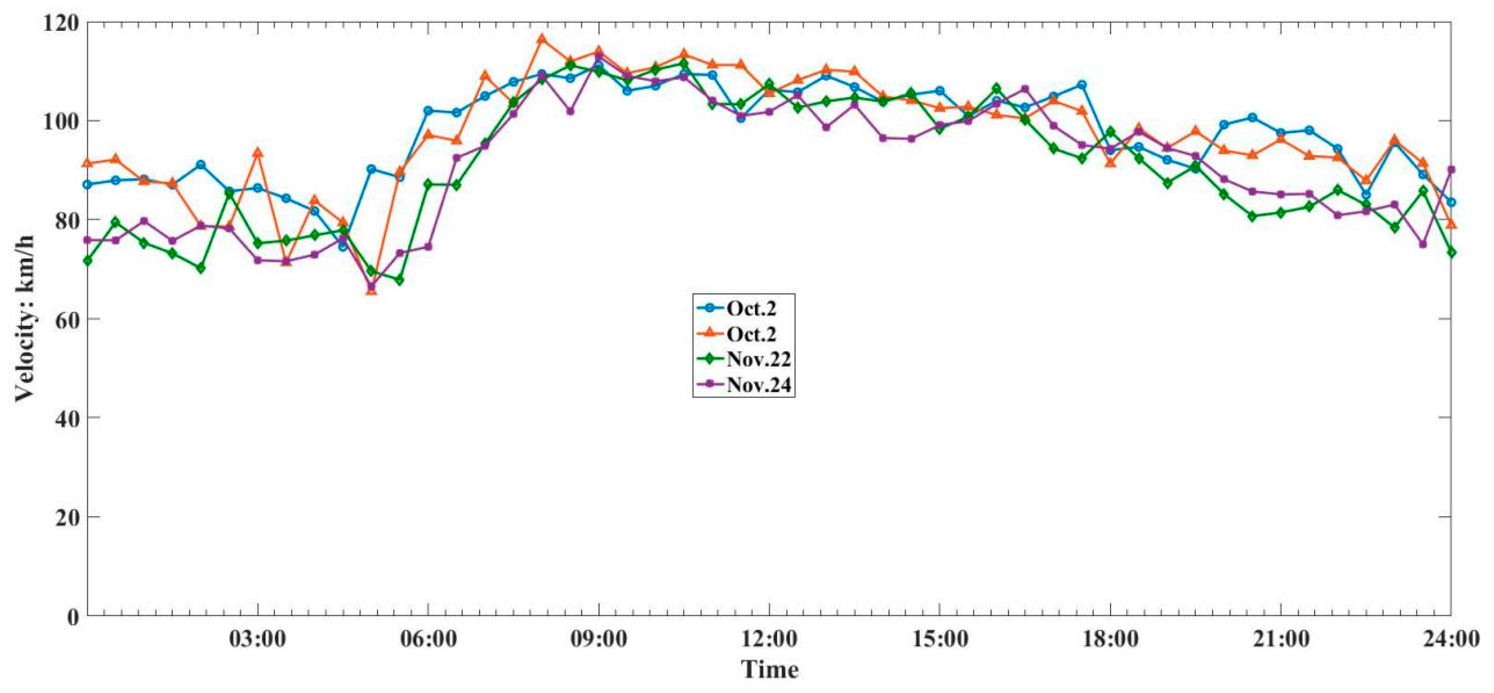
3.1. Data Relevance Analysis

Due to the regularity of daily travel behavior, the traffic data collected from the same sensor presents the temporal similarities [39]. To illuminate the relevance of data, field velocity data collected from the same sensor are shown in Figure 1 presenting highway traffic velocity data 24h a day for four days in Shandong, China. In this section, the velocity data are randomly selected from the history database. Table 1 presents the Pearson correlation between different day data in an environment. The correlation index is greater than 0.8, reaching a very significant degree. All the results are in excellent agreement with the experimental data reported by Heng et al. [39]. Therefore, the normal historical data can be used for recovering the abnormal data.

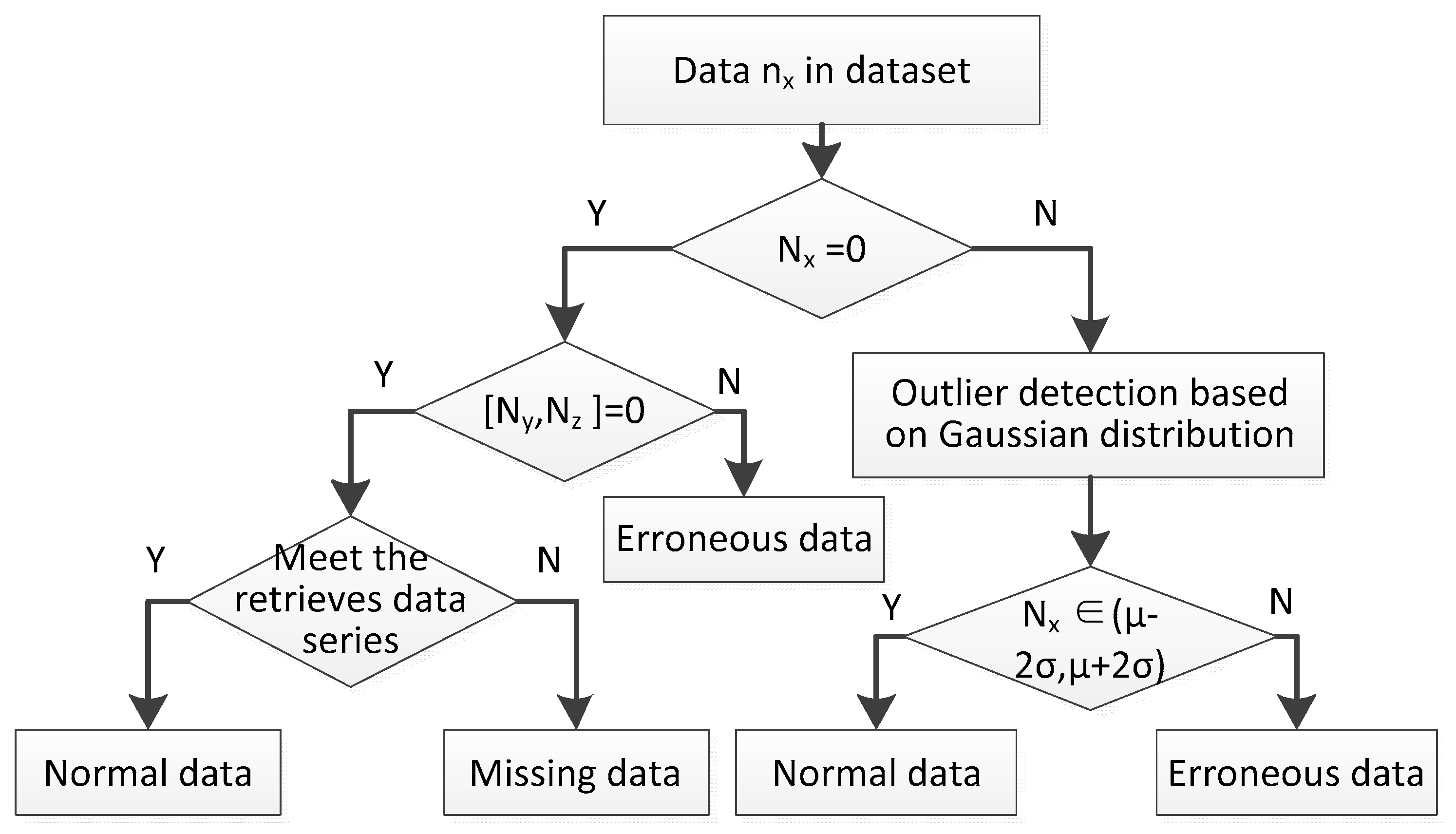
3.2. Abnormal Data Identification

Abnormal data are unreasonable values in the dataset. Abnormal data, once regarded as noisy data in statistics, have turned out to be an important problem, which is being researched in diverse fields of research and application domains [40]. Abnormal data arise due to mechanical faults, changes in the system behavior, fraudulent behavior, human error, instrument error, or simply through natural deviations in populations [41,42]. Actually, several normal data are similar with the abnormal data, but which can provide very useful information. For example, the absence of data may be considered as a missing case or a sample zero. The identification of the abnormal data is a prerequisite for the data recovery. Hence, a simple approach is proposed to determine the type of data. Note that the abnormal data is defined as the outlier, involving the missing data and the erroneous data. Furthermore, the abnormal data identification framework is shown in Figure 2.
Figure 2 shows the main process of identifying the abnormal data. The detailed information can be depicted as follows.
Step 1. The data N x should be judged whether the value equals 0. If the value is 0, Step 2 is executed; otherwise, go to Step 5.
Step 2. The correlation parameters N y and N z are judged whether the value is equal to 0. If N y = 0 and N z = 0 , Step 4 is executed; otherwise, go to Step 3. Specifically, the correlation parameters generally include velocity, density (or occupancy), and traffic flow.
Step 3. N x is erroneous data.
Step 4. In order to avoid the erroneous judgment, the data series will be further identified when N x = 0 , N y = 0 , N z = 0 . The retrieved data series in correlation time series should be checked. If the match is high, the N x is defined as the normal data; otherwise, N x is a missing data.
Step 5. Traffic data have spatiotemporal correlation and similar tendency. Abnormal data detection based on Gaussian distribution will be performed. Furthermore, Step 6 is executed.
Step 6. If the N x belongs to the scope ( μ x 2 σ x , μ x + 2 σ x ) , the N x is normal data; otherwise, N x is erroneous data. Specifically, μ x is the mean value of the N x in the time series and σ x is the standard deviation.
Remark 1.
Abnormal data detection based on the Gaussian distribution is a popular method [43]. The main idea can be described through a simple statement. First, the assumption is that there are m points(J_1, …, J_m). Then, the mean value μ_J and standard deviation σ_J can be calculated, shown by Equations (1) and (2), separately.
μ J = i = 1 m J i m
and
σ J = i = 1 m ( J i μ J ) 2 m
Under the assumption of normal distribution, the scope ( μ J 2 σ J ,   μ J + 2 σ J ) includes 99.7% of the data. If the distance between J i and μ J is beyond 2 σ J , J i is an abnormal data; otherwise, J i is a normal data.
Table 2 shows the field data obtained from a loop coil sensor with an interval of 1 min. In addition, although the velocity data present zero at time 1:03, 1:07, and 1:14, the traffic flow and occupancy are not equal zero. According to the process of abnormal data identification presented in Figure 2, these data can be defined as erroneous data.

4. Basic KNN Algorithm

The KNN nonparametric regression method is a widely applied nonparametric regression algorithm, with many advantages, such as no parameters, a small error ratio, and a wide error distribution. At present, the KNN algorithm has been mainly applied to traffic flow prediction. With the difference in the parameter adjustment rules, the improvement in KNN will be proposed in the next section. The main parameters of the KNN are described as follows.

4.1. Nearest Neighbor

The nearest neighboring K presents the number of neighbors selected from the historical set. The quality of the historical set affects the K value. Regardless of if the K value is too large or too small, the accuracy of the data recovery can be affected. Because there is no guiding principle, the studies in the existing literature used their own experimental data to find better values.

4.2. State Vector

As a criterion for matching the current data with the historical set, the state vector is a set of characteristic data used for matching the algorithm parameters when searching for neighbors. The result of the state vector selection will affect the accuracy of the recovery method.

4.3. Distance Measurement Method

In general, Euclidean distance and Manhattan distance are the most popular distance calculation methods. Manhattan distance is limited by the dimensions with considering the actual impedance. In detail, Manhattan distance only calculates the horizontal or vertical distance between two points in the plane, also called the CityBlock distance. However, most of the data is not just two-dimensional and are distributed in different dimensions. Euclidean distance can be applied to the distances of multiple dimension calculations. Therefore, the Euclidean distance is selected as the similarity measure in the conventional KNN algorithm, which usually relates to all the attributes. Equation (3) shows the Euclidean distance between two sequences X and Y , where X = ( x 1 , x 2 , , x n ) a n d   Y = ( y 1 , y 2 , , y n ) .
d X Y = i = 1 n ( x i y i ) 2

4.4. Recovery Algorithm

According to the calculation results of Euclidean distance, K groups of nearest neighbor data would be obtained. Note that each group is a state vector. In KNN, the feature state vector including abnormal data as the basic unit is used for tracking the similar state vector. Furthermore, the abnormal data recovery value can be given by Equation (4).
v ^ ( w ) = i = 1 k α i v h i ( w )
where v h i ( w ) is the sub data in the group i data in the history database, α i is the weight of the subdata in the i -th data in the historical set, and v ^ ( w ) is the recovered value of the abnormal data.

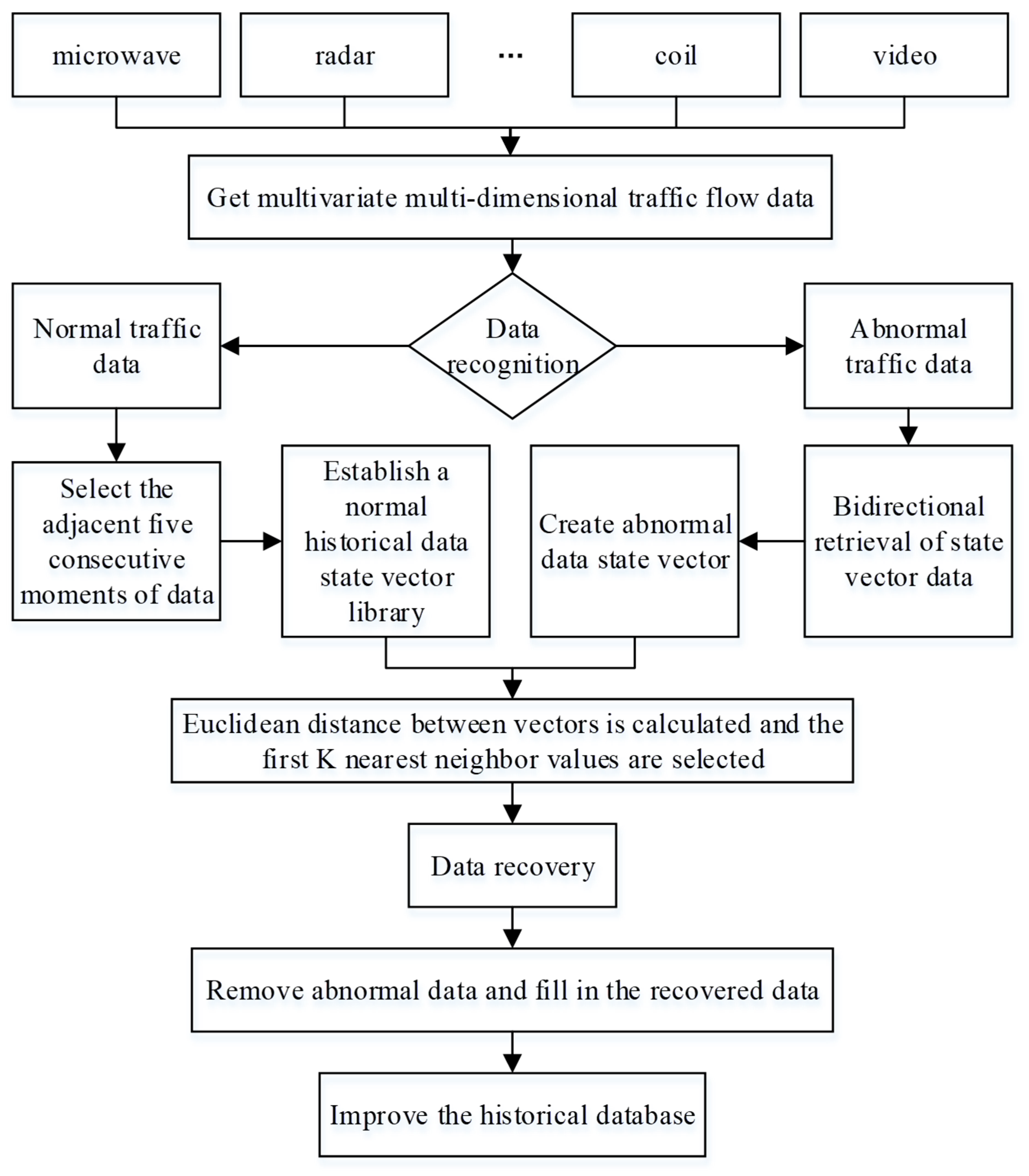
5. Bidirectional Data Recovery Approach

A bidirectional data recovery approach is proposed in this paper, aiming to improve data quality, based on the KNN algorithm and the bidirectional retrieval principle. The main changes of the proposed recovery approach can be summarized as three points. First, an appropriate K value is selected by analyzing the relationship between the recovery accuracy and the number of the nearest neighbor values. Second, the feature state vector is designed considering the bidirectional retrial principle. In detail, the state vector consists of five consecutive data. Third, a suitable neighbor weight value is selected to improve the data recovery accuracy. The data recovery process is illustrated in Figure 3.

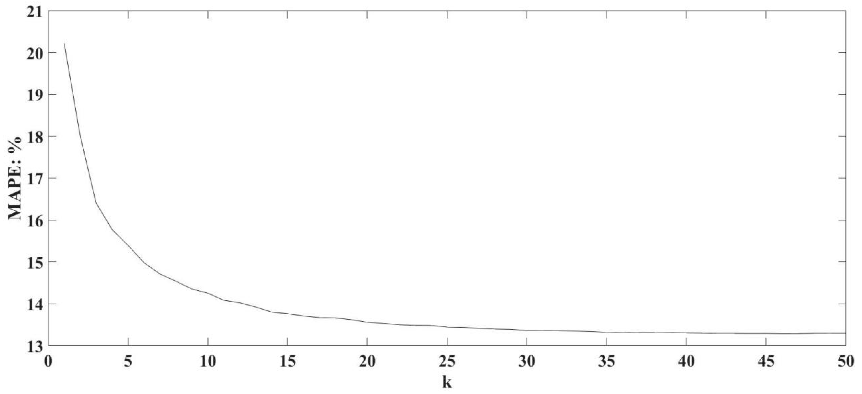
5.1. Parameter K Selection

To select the optimal nearest neighbor value, the relationship between the mean relative error of the data recovery and the change in K is analyzed, as shown in Figure 4, where K ranges from 1 to 50. In Figure 4, there are 1440 data points are used. In the beginning, the average relative error value will decrease with increasing K value. When the K equals about 25, the change in the average relative error value tends to converge. This result is consistent with the experiment that the optimal K value is between 20 and 25 as reported by Turochy [44]. Therefore, the K equals 25 was applied in this proposed bidirectional data recovery approach for preventing excessive convergence and unnecessary operation.

5.2. Designed State Vector

In the conventional KNN algorithm, the state vector is designed considering the correlation between the estimated data and the unidirectional time series. However, in the data recovery field, the bidirectional correlation in the time dimension should be paid more attention. Hence, the bidirectional abnormal data state vector was proposed and is presented in this section.

5.2.1. Historical Data Status Vector Library

For the continuous traffic flow data from the same sensor, there is a strong correlation among the adjacent data illuminated in Section 3.1. Therefore, five consecutive data as a group of historical data state vector library were established as X n ,   X n = { v h 1 i , v h 2 i , v h 3 i , v h 4 i , v h 5 i }   ( i = 1 , 2 , , n ) . . In addition, the historical data state vector library can be expressed as Equation (5).
X n = [ X 1 X 2 X 3   X n ] = [ v h 1 1 v h 2 1 v h 3 1 v h 4 1 v h 5 1 v h 1 2 v h 2 2 v h 3 2 v h 4 2 v h 5 2 v h 1 3 v h 2 3 v h 3 3 v h 4 3 v h 5 3 v h 1 n v h 2 n v h 3 n v h 4 n v h 5 n ]

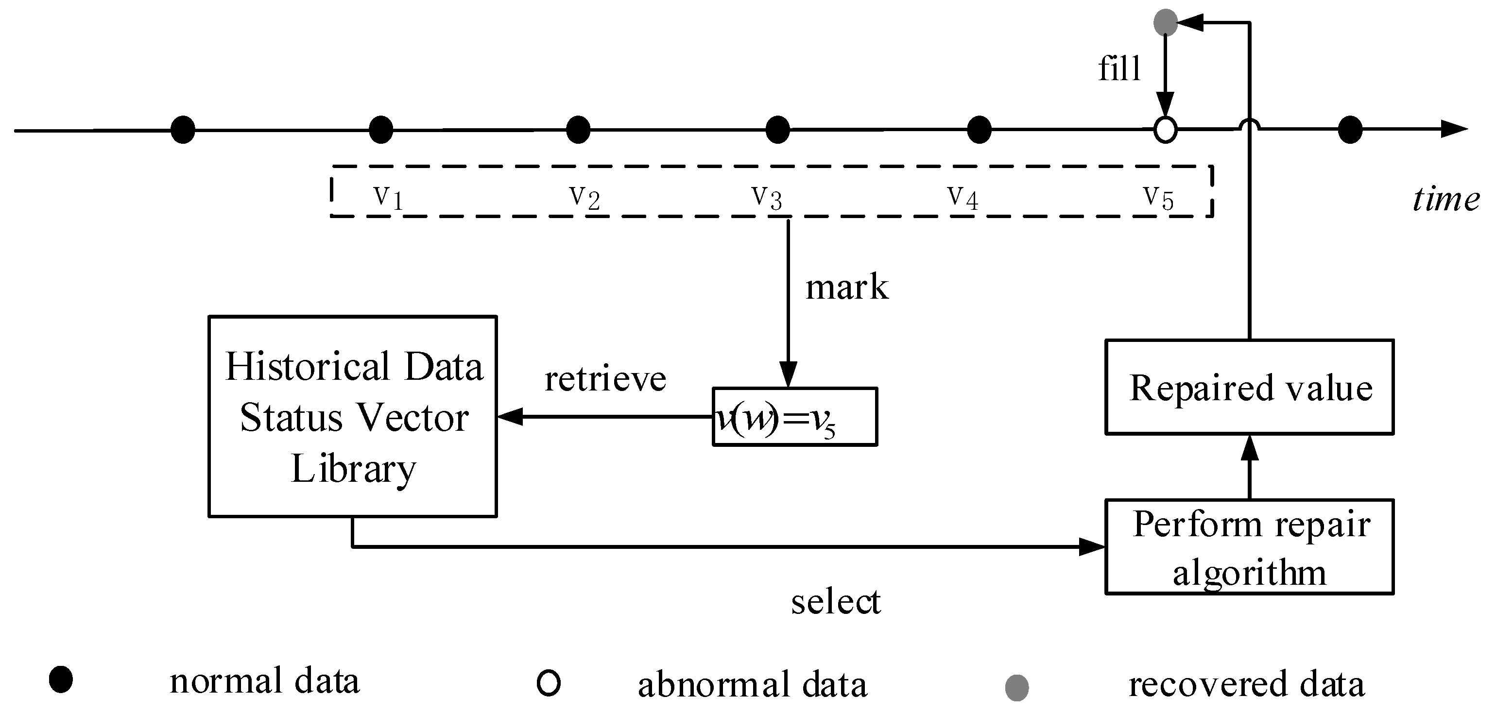
5.2.2. Unidirectional abnormal data state vector

In order to explicit the advantage of the bidirectional recovery approach, it is necessary to introduce the process of the unidirectional state vector building in the conventional KNN (Uni-KNN). According the unidirectional principle, the abnormal state vector is shown as X u = { v 1 i , v 2 i , v 3 i , v 4 i , v 5 i } (i = 1, 2, …, n), where v 5 i is the abnormal data. Therefore, the state vector can be expressed as X u = { v 1 i , v 2 i , v 3 i , v 4 i , v ( w ) } , where   v ( w ) = v 5 i . The basic thought of Uni-KNN is illustrated in Figure 5.

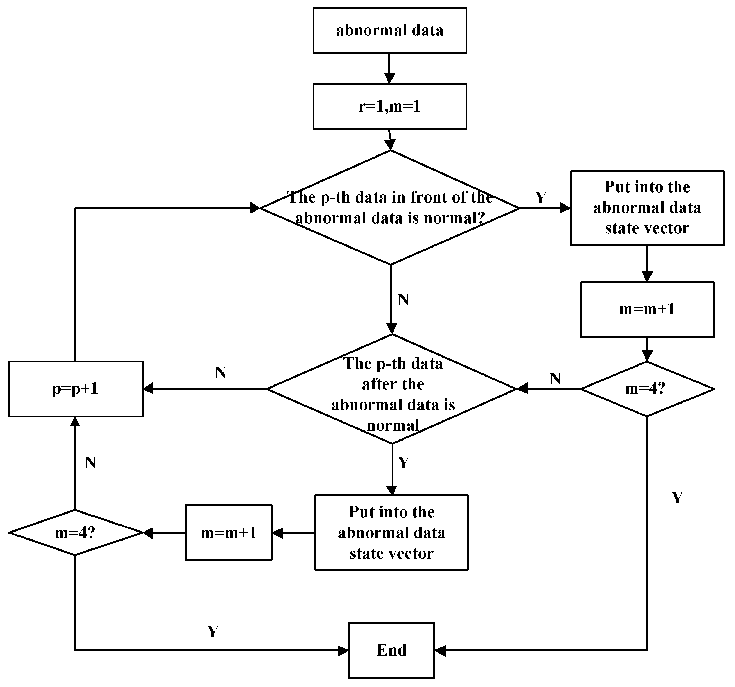
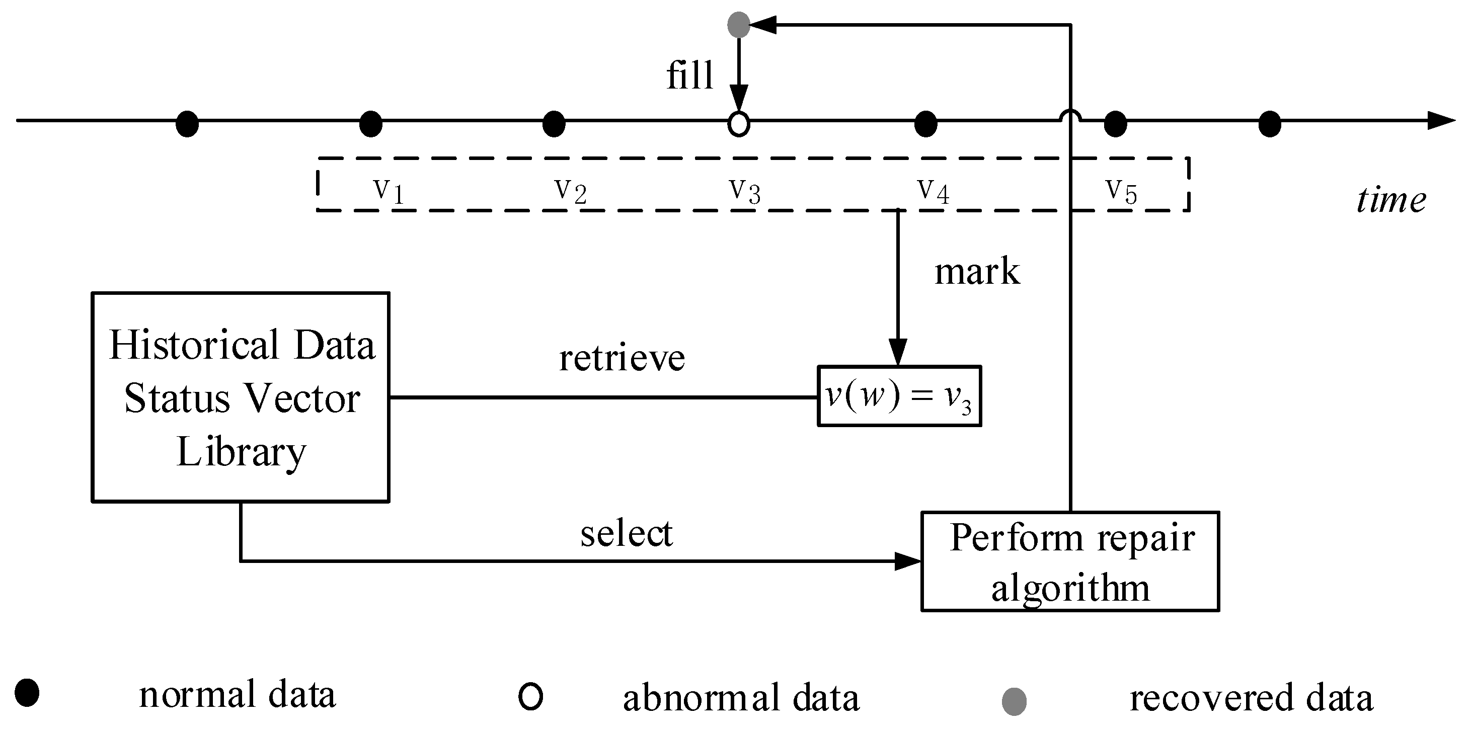
5.2.3. Bidirectional Abnormal Data State Vector

The bidirectional symmetry search concept is introduced to construct the state vector in the proposed bidirectional recovery approach, which considers the correlations between the abnormal data and the adjacent data. Hence, the proposed approach is also called Bid-KNN. During the searching process of the abnormal data, the abnormal data state vector can be seen as a particle, which keeps looking for the similar symmetric particles among the vector groups. The similar symmetric vectors have the same data number and higher similarity among the database. With the correlation among traffic data, the state vector can be constructed as X b = { v 1 , v 2 , v 3 , v 4 , v 5 } . Abnormal data v ( w ) . can be any one of these five values. In detail, the building process of the state vector is shown as follows.
The abnormal data are detected and marked as v ( w ) . First, the data at the previous moment is retrieved. If it is normal data, it is placed in the state vector X b ; otherwise, retrieve the next moment data of the data v ( w ) . If the next moment data of the data v ( w ) is normal data, it is placed in the state vector X b , else search for the next data. Based on the search rules, the data are sequentially retrieved until the four normal data of the adjacent time periods of the abnormal data are achieved. Finally, the abnormal data state vector X b would be established. The state vector is defined as X b = { v 1 i , v 2 i , v 3 i , v 4 i , v 5 i } (i = 1, 2, …, n). According to the above criterion, the place of the abnormal data in state vector is random. For description, it assumed that v 3 is abnormal data, where v ( w ) = v 3 i . The abnormal data symmetric state vector can be expressed as X b = { v 1 i , v 2 i , v ( w ) , v 4 i , v 5 i } . and the establishment process of the bidirectional abnormal data state vector is shown in Figure 6. The bidirectional data recovery process is illustrated in Figure 7.

5.3. Weight Assignment

The accuracy of data recovery was improved by applying a method of weighting the neighbors. The nearer the distance is, the greater weight assigned. The common weight assignment methods include the (1) equal weights method (all candidates are given the same weight), (2) inverse distance weight method [45] (a type of deterministic method used in this paper to assign the weight values based on the neighborhood locations), and (3) rank-based weights method (the weight is given by the rank of the candidates classified by the distance from the subject profile). The inverse distance and rank-based weighting methods are better than the equal distance weighting method for identifying similar traffic patterns [46]. Therefore, the inverse distance weight (I-d) and rank-based (R-b) methods of weight assignment were used in this paper and can be expressed by Equations (6) and (7), respectively.
α i = d i 1 i = 1 k d i 1
and
α i = ( k i + 1 ) 2 i = 1 k ( k i + 1 ) 2
where i is the rank of the i-th candidate, k is the total number of candidates, d i is the Euclidean distance between the current data and the i -th data in the historical set, and α i is the weight of the i -th neighbor value.

6. Experiment and Results

6.1. Performance Evaluation

The recovery accuracy and efficiency were quantitatively measured using the indicators for the root mean standard error (RMSE), mean absolute percentage error (MAPE), and the correlation coefficient r. Expressed by Equation (8), RMSE is the standard deviation of the errors, measuring the deviation between the real values and recovery values.
R M S E = i = 1 n ( v ^ i ( w ) v i ) 2 n
where v i is the real value, v ^ i ( w ) is the i-th recovered value, and n is the number of abnormal values.
Expressed by Equation (9), MAPE provides the accuracy of the method and shows the difference between the real and recovered data values.
M A P E = 1 n i = 1 n | v ^ i ( w ) v i v i | × 100 %
The correlation coefficient r measures the linear similarity between the recovered and real data and its ranges between −1 and 1. The absolute value of r relates to the strength of the relationship. A value closes to 1 indicates a strong predictive capability. The formula is given by equation (10), where v ¯ is the mean of v i and v ^ ( w ) ¯ is the mean of v ^ i ( w ) .
r = i = 1 n ( v i v ¯ ) ( v ^ i ( w ) v ^ ( w ) ¯ ) ( i = 1 n ( v i v ¯ ) 2 i = 1 n ( v ^ i ( w ) v ^ ( w ) ¯ ) 2 ) 1 2

6.2. Experimental Design
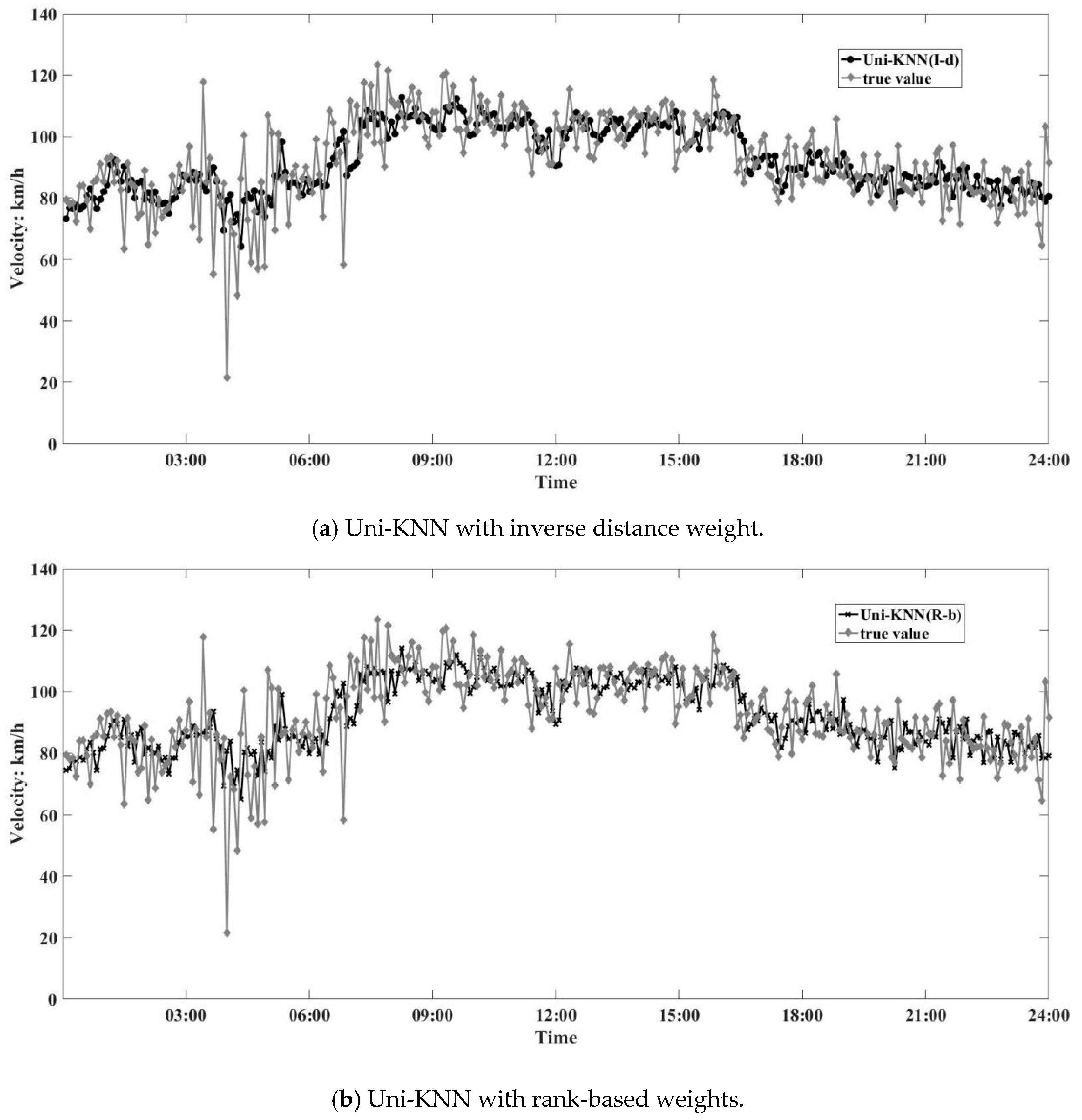
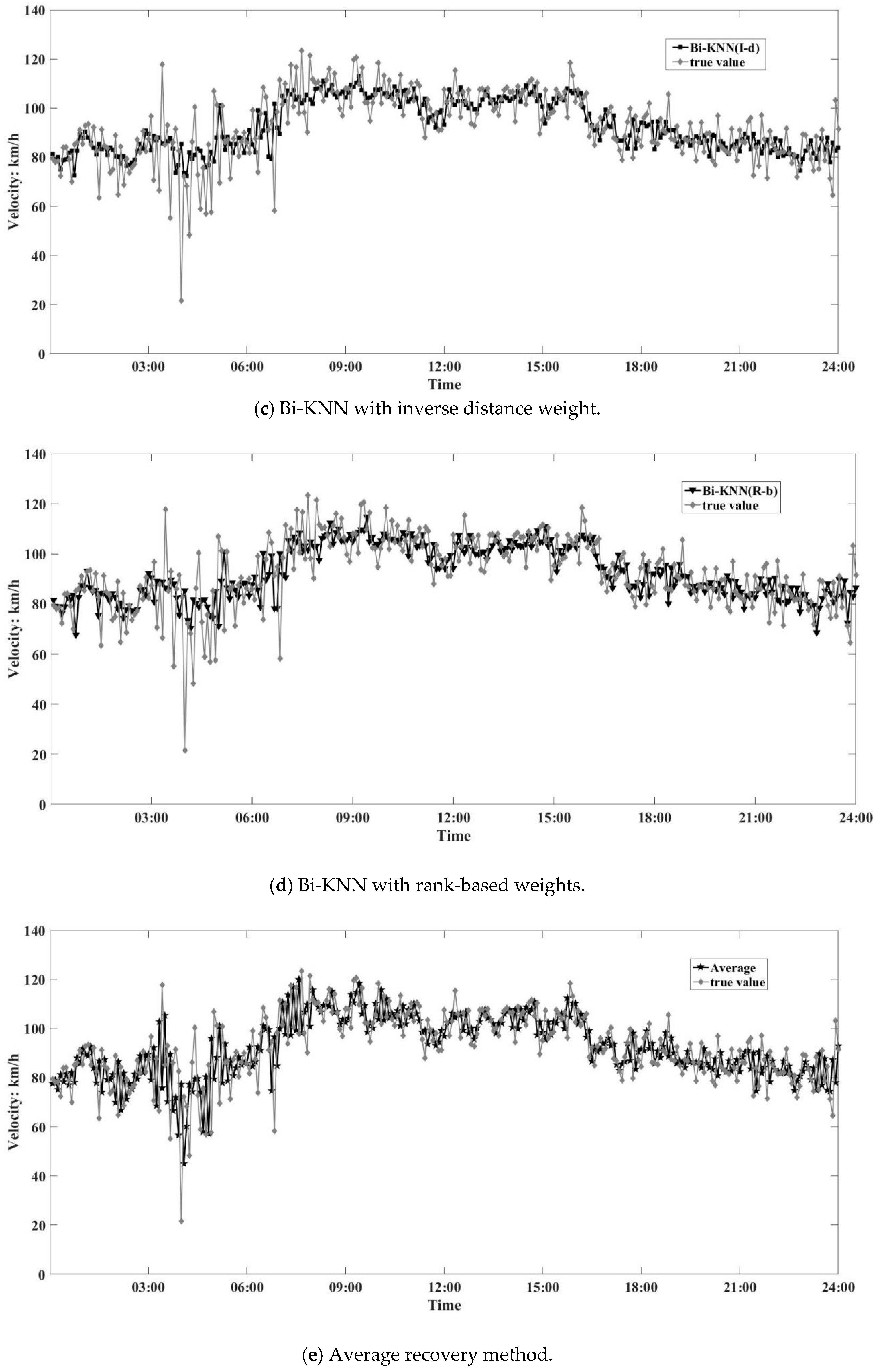
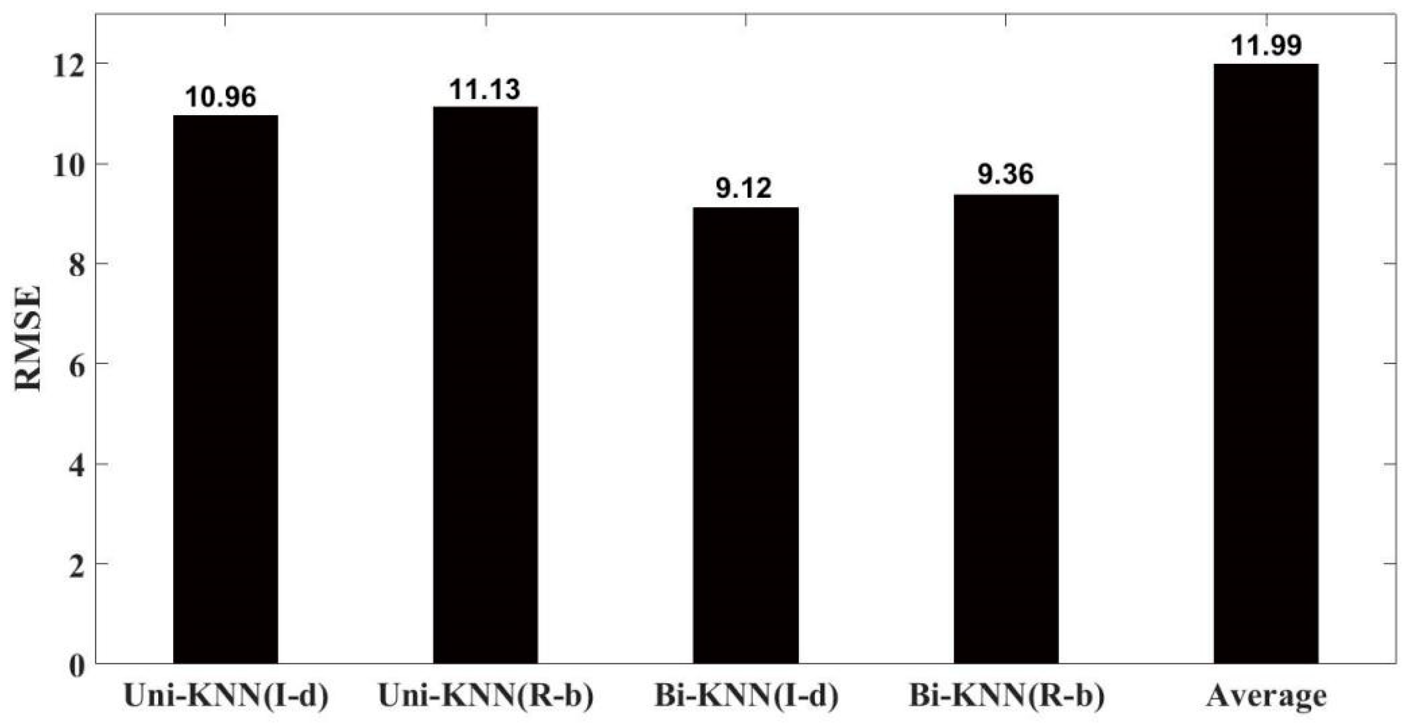
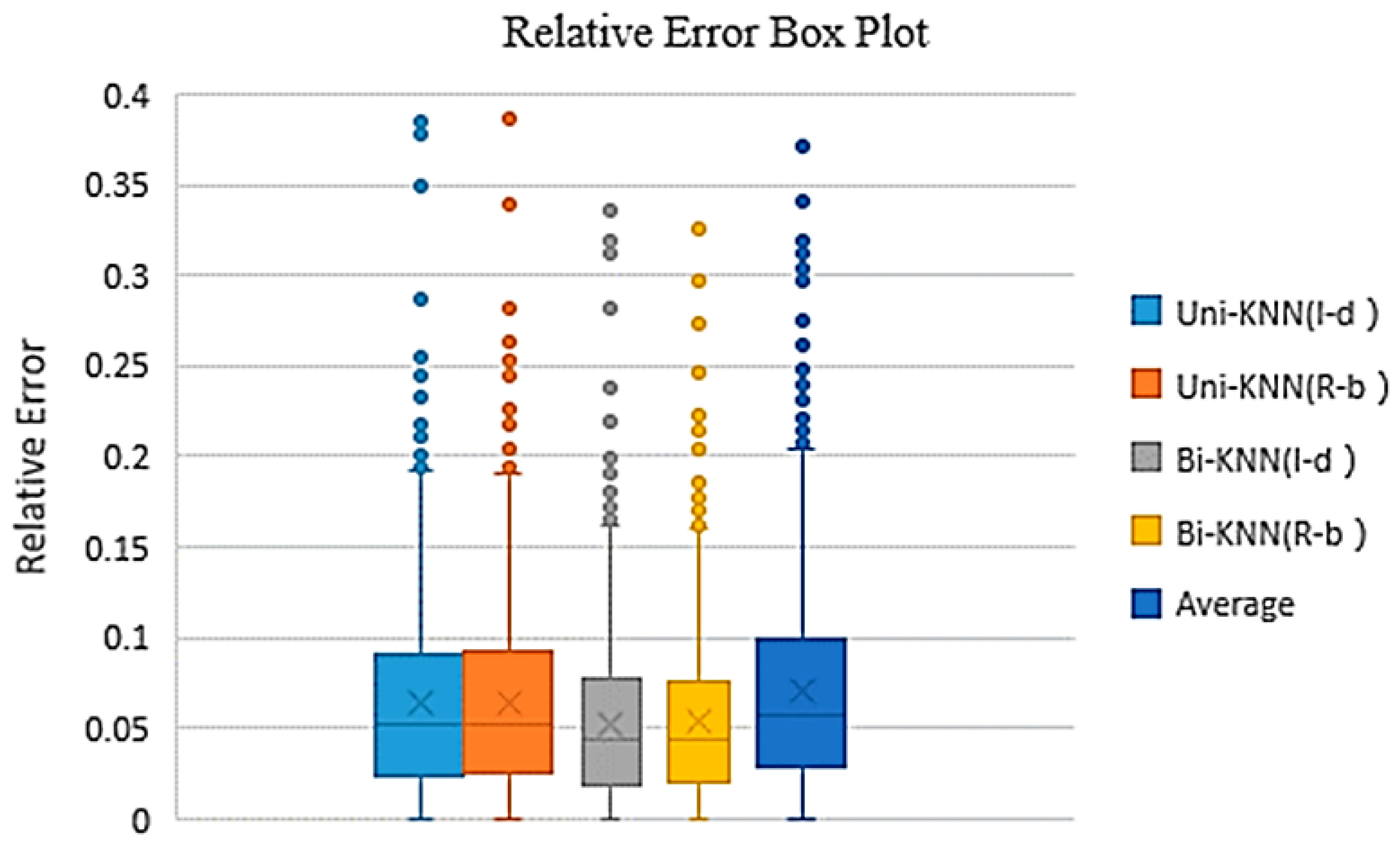
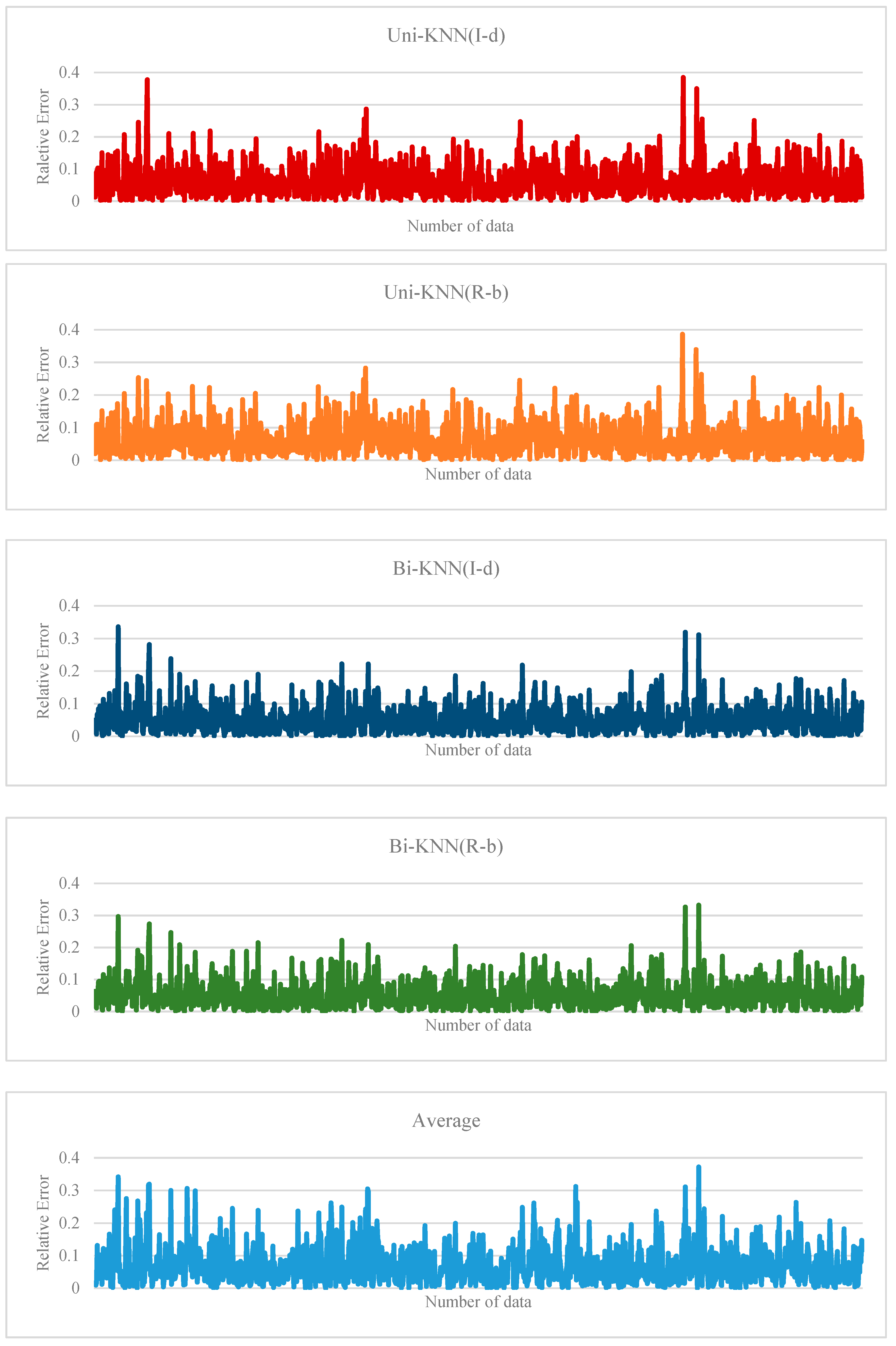
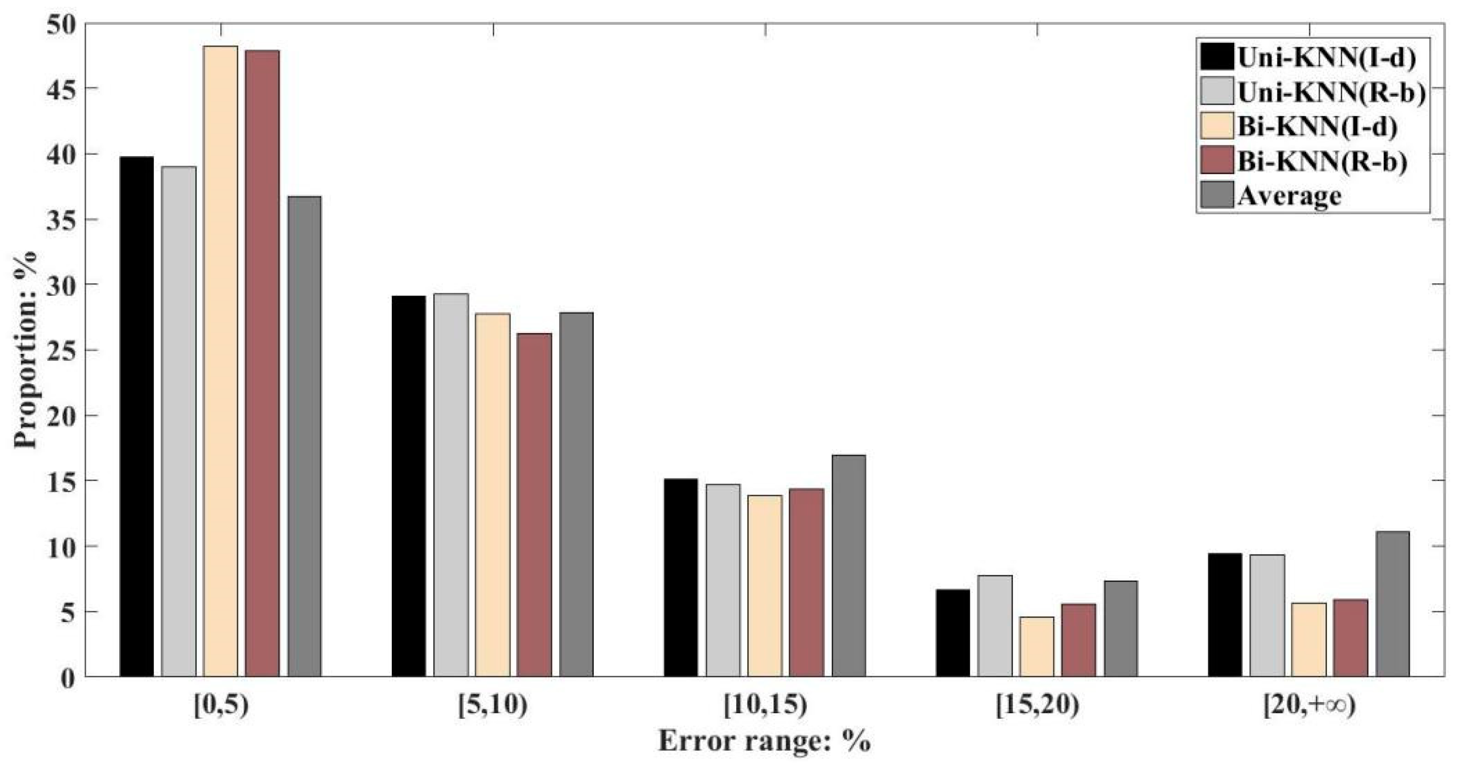
Abnormal data is recovered using the field velocity data, which is known to be accurately exhibiting traffic conditions when compared to out parameters in ITS. For verifying the validity of the proposed approach, the data over six normal days were selected as the test data and any one of the data in the test set could be the abnormal data. Collecting field data is essential for recovering the abnormal data. This paper uses the field velocity data from Shandong, China. To reflect the traffic condition better, the velocity data (aggregated at 5 min) of 60 consecutive days as a sample of experimental data are adopted to verify the effectiveness of the proposed data recovery approach. The database is divided into two categories: historical set and test set. In detail, 54 days of data are selected as the historical data and the last 6 days of data were selected as the test data. The data from sensor were collected during the full day (0:00–24:00).
The multiple sets of velocity data were used for experimental verification, affording consistent results. In order to avoid repeating descriptions, one set of the experimental result is shown in this section. In the process of experiment, in order to evaluate the performance of the recovery method, five recovery methods, including the traditional averaging recovery method, Uni-KNN using inverse distance weight (Uni-KNN (I-d)), Uni-KNN using rank-based weight (Uni-KNN(R-b)), Bi-KNN using inverse distance weight (Bi-KNN (I-d)), and Bi-KNN using rank-based weight (Bi-KNN (R-b)) were compared.

6.3. Results

The accuracies of five methods were compared. The overall situation is presented in Figure 8, showing the RMSE, MAPE, and correlation coefficient r of the five recovery methods and the true value recovered throughout the whole day. In general, the Bi-KNN recovery methods exhibited low errors (Figure 8c,d) compared to the Uni-KNN recovery methods (Figure 8a,b). The averaging method exhibits a higher error among the five recovery methods.
RMSE measures the error between the true value and the recovery value. A smaller error indicates better performance. Figure 9 shows the RMSE and the difference among the five recovery methods. A significant difference is shown in Figure 9, indicating a good recovery outcome of the Bi-KNN and Uni-KNN in abnormal data compared to the traditional averaging method. The RMSE of the traditional averaging method reaches 11.99% on average. The accuracy of Bi-KNN is higher than that of the Uni-KNN. The accuracy of Bi-KNN adopting the inverse distance weight is higher than that of Uni-KNN adopting the inverse distance weight.
The relative error value is an evaluation indicator of the error. A smaller relative error value indicates a better performance. Figure 10 shows the relative errors of the five methods used in this paper. It is calculated by the difference in the results of recovery method and the true value. A comparison of the five methods showed better performance of the Bi-KNN than others.
The relative error distributions are shown in Figure 11. As shown in Figure 11, the relative errors value of the Bi-KNN and Uni-KNN methods are obviously lower than that of the traditional averaging method. The effectiveness of the proposed algorithm is demonstrated. Moreover, the relative error of the Bi-KNN method is lower than that of the Uni-KNN method. By comparing the results of the relative error, the availability of the Bi-KNN was further determined.
Figure 12 shows the relative errors of the five comparison methods, and the abscissa values are presented as (0, 5%), (5%, 10%), (10%, 15%), (15%, 20%), and (20%, + ∞). As shown in Figure 12, the relative error ratio of Bi-KNN is lower than 5%. Bi-KNN shows a good performance to recover the abnormal data compared to other methods. In detail, approximately 50% relative recovery errors are belonging in the ranges from 0 to 5%. The performance of the relative errors of Bi-KNN is superior to that of the Uni-KNN.
Table 3 presents the correlation coefficients r calculated by the five comparison methods. The correlation coefficient r indicates the degree of similarity between the true data and recovery data. The greater the correlation coefficient value, the more accurate recovery is. To evaluate the efficiency, it is necessary to analyze the correlation coefficient between the recovery value and the true value. As listed in Table 3, the correlation coefficients of Bi-KNN and Uni-KNN are significantly greater than that of the traditional averaging method. Moreover, the correlation coefficients of the Bi-KNN are greater than that of the Uni-KNN. In the bidirectional recovery methods, the Bi-KNN model adopting the inverse distance weight has the greatest correlation coefficient 0.8033, indicating that Bi-KNN(I-d) performs the most accurate recovery compared to other comparison methods.

7. Conclusions

An accurate method was designed for improving data quality. Based on the KNN algorithm, a novel bidirectional k-nearest neighbor searching method was developed to recover the abnormal data existing in the database. In the test case, the field data were used to verify the efficiency of five recovery methods including the traditional averaging recovery method, Uni-KNN using inverse distance weight (Uni-KNN (I-d)), Uni-KNN using rank-based weight (Uni-KNN(R-b)), Bi-KNN using inverse distance weight (Bi-KNN (I-d)), and Bi-KNN using rank-based weight (Bi-KNN (R-b)). The data interval was set to 5 min. The test results show that the bidirectional recovery method is very effective for repairing the abnormal data with a low RMSE. Moreover, the relative errors of the five comparison methods indicate that the Bi-KNN (I-d) is more accurate and has a good efficiency. The correlation coefficient of the Bi-KNN (I-d) is 0.8033, which is greater than those of the other methods. Overall, the proposed Bi-KNN (I-d) has higher recovery accuracy, and the results are relatively satisfactory. This method could meet the demand for the precise restoration of basic anomalous data and improve the quality of traffic data effectively.
The abnormal traffic flow data recovery method considers the missing and the erroneous data. In the future, different proportion of existing abnormal data will be considered and different models will be applied to further enhance the accuracy of the recovery method. Moreover, a more symmetrical time–space network will be considered to improve the model accuracy and extend the scope of application in the further work.

Author Contributions

Conceptualization, M.M. and S.L.; methodology, Y.Q.; software, Y.Q.; validation, M.M., S.L. and Y.Q.; formal analysis, S.L.; investigation, Y.Q.; resources, M.M. and S.L.; data curation, M.M.; writing—original draft preparation, M.M. and Y.Q.; writing—review and editing, M.M. and S.L.; visualization, M.M.; supervision, M.M.; project administration, M.M. and S.L.; funding acquisition, M.M. and S.L.

Funding

This research was funded by “National Natural Science Foundation of China, grant number 71801149, 71801153, and 71601118”, “the Technical Service Platform for Vibration and Noise Testing and Control of New Energy Vehicles, grant number 18DZ2295900”, and “the Shanghai Municipal Natural Science Foundation, grant number 14ZR1418600“.

Conflicts of Interest

The authors declare no conflicts of interest.

Nomenclature

KNumber of candidate values
i Rank of the i-th candidate
d i Distance between the current data and the group i data in the historical set
α i Weight of subdata in the i-th data in the historical set
v ^ ( w ) Recovered value of abnormal data
v i Real value.
v ¯ Mean of v i
v ^ i ( w ) i-th recovered value
v ^ ( w ) ¯ Mean of v ^ i ( w )
nNumber of abnormal value

References

  1. Guo, M.; Lan, J.; Li, J.; Lin, Z.; Sun, X. Traffic flow data recovery algorithm based on gray residual GM (1, N) model. J. Transp. Syst. Eng. Inf. Technol. 2012, 12, 42–47. [Google Scholar] [CrossRef]
  2. Ma, M.; Liang, S. An integrated control method based on the priority of ways in a freeway network. Trans. Inst. Meas. Control 2018, 40, 843–852. [Google Scholar] [CrossRef]
  3. Ma, M.; Liang, S. An optimization approach for freeway network coordinated traffic control and route guidance. PLoS ONE 2018, 13. [Google Scholar] [CrossRef] [PubMed]
  4. Chen, H.; Margaret, B. Instrumented city database analysts using multi-agents. Transp. Res. Part C Emerg. Technol. 2002, 10, 419–432. [Google Scholar] [CrossRef]
  5. Liang, S.; Ma, M. Analysis of bus bunching impact on car delays at signalized intersections. KSCE J. Civ. Eng. 2019, 23, 833–843. [Google Scholar] [CrossRef]
  6. Liang, S.; Ma, M.; He, S.; Zhang, H.; Yuan, P. Coordinated control method to self-equalize bus headways: An analytical method. Transportmetrica B Transp. Dyn. 2019, 7, 1175–1202. [Google Scholar] [CrossRef]
  7. Zhang, J.; el Kamel, A. Virtual traffic simulation with neural network learned mobility model. Adv. Eng. Softw. 2018, 115, 103–111. [Google Scholar] [CrossRef]
  8. Duan, Y.; Lv, Y.; Liu, Y.; Wang, F. An efficient realization of deep learning for traffic data imputation. Transp. Res. Part C Emerg. Technol. 2016, 72, 168–181. [Google Scholar] [CrossRef]
  9. Sharma, S.; Lingras, P.; Zhong, M. Effect of missing values estimations on traffic parameters. Transp. Plan. Technol. 2004, 27, 119–144. [Google Scholar] [CrossRef]
  10. Ma, M.; Liang, S.; Guo, H.; Yang, J. Short-term traffic flow prediction using a self-adaptive two-dimensional forecasting method. Adv. Mech. Eng. 2017, 9, 168781401771900. [Google Scholar] [CrossRef]
  11. Patil, D.V.; Bichkar, R.S. Multiple imputation of missing data with genetic algorithm based techniques. IJCA Spec. Issue Evol. Comput. Optim. Tech. 2010, 74–78. [Google Scholar]
  12. Van Lint, J.W.C.; Hoogendoorn, S.P.; van Zuylen, H.J. Accurate freeway travel time prediction with state-space neural networks under missing data. Transp. Res. Part C Emerg. Technol. 2005, 13, 347–369. [Google Scholar] [CrossRef]
  13. Silva-Ramírez, E.-L.; Pino-Mejías, R.; López-Coello, M. Missing value imputation on missing completely at random data using multilayer perceptrons. Neural Netw. Off. J. Int. Neural Netw. Soc. 2011, 24, 121–129. [Google Scholar] [CrossRef]
  14. Bálint, D.; Jäntschi, L. Missing data calculation using the antioxidant activity in selected herbs. Symmetry 2019, 11, 779. [Google Scholar] [CrossRef]
  15. Laña, I.; Olabarrieta, I.I.; Vélez, M.; Del Ser, J. On the imputation of missing data for road traffic forecasting: New insights and novel techniques. Transp. Res. Part C Emerg. Technol. 2018, 90, 18–33. [Google Scholar] [CrossRef]
  16. Yan, Y.; Zhang, S.; Tang, J.; Wang, X. Understanding characteristics in multivariate traffic flow time series from complex network structure. Phys. A Stat. Mech. App. 2017, 477, 149–160. [Google Scholar] [CrossRef]
  17. Pushkar, A.; Hall, F.L.; Acha-Daza, J.A. Estimation of speeds from single-loop freeway flow and occupancy data using cusp catastrophe theory model. Transp. Res. Rec. 1994, 1457, 149–157. [Google Scholar]
  18. Chen, J.; Shao, J. Nearest neighbor imputation for survey data. J. Off. Stat. 2000, 16, 113–131. [Google Scholar]
  19. Yuan, K.H.; Marshall, L.L.; Bentler, P.M. A unified approach to exploratory factor analysis with missing data, nonnormal data, and in the presence of outliers. Psychometrika 2002, 67, 95–121. [Google Scholar] [CrossRef]
  20. Troyanskaya, O.; Cantor, M.; Sherlock, G.; Brown, P.; Hastie, T.; Tibshirani, R.; Botstein, D.; Altman, R.B. Missing value estimation methods for DNA microarrays. Bioinformatics 2001, 17, 520–525. [Google Scholar] [CrossRef] [Green Version]
  21. Smith, B.; Scherer, W.; Conklin, J. Exploring Imputation techniques for missing data in transportation management systems. Transp. Res. Rec. J. Transp. Res. Board 2003, 1836, 132–142. [Google Scholar] [CrossRef]
  22. Chen, C.; Kwon, J.; Rice, J.; Skabardonis, A.; Varaiya, P. Detecting errors and imputing missing data for single-loop surveillance systems. Transp. Res. Rec. J. Transp. Res. Board 2003, 1855, 53–57. [Google Scholar] [CrossRef]
  23. Abdella, M.; Marwala, T. The use of genetic algorithms and neural networks to approximate missing data in database. In Proceedings of the IEEE 3rd International Conference on Computational Cybernetics, Mauritius, 13–16 April 2005; pp. 207–212. [Google Scholar]
  24. Tang, J.; Zhang, G.; Wang, Y.; Wang, H.; Liu, F. A hybrid approach to integrate fuzzy C-means based imputation method with genetic algorithm for missing traffic volume data estimation. Transp. Res. Part C Emerg. Technol. 2015, 51, 29–40. [Google Scholar] [CrossRef]
  25. Min, W.; Wynter, L. Real-time road traffic prediction with spatio-temporal correlations. Transp. Res. Part C Emerg. Technol. 2011, 19, 606–616. [Google Scholar] [CrossRef]
  26. Aydilek, I.B.; Arslan, A. A novel hybrid approach to estimating missing values in databases using k-nearest neighbors and neural networks. Int. J. Innov. Comput. Inf. Control 2012, 8, 4705–4717. [Google Scholar]
  27. Lobato, F.; Sales, C.; Araujo, I.; Tadaiesky, V.; Dias, L.; Ramos, L.; Santana, A. Multi-objective genetic algorithm for missing data imputation. Pattern Recognit. Lett. 2015, 68, 126–131. [Google Scholar] [CrossRef]
  28. Bae, B.; Kim, H.; Lim, H.; Liu, Y.; Han, L.D.; Freeze, P.B. Missing data imputation for traffic flow speed using spatio-temporal cokriging. Transp. Res. Part C Emerg. Technol. 2018, 88, 124–139. [Google Scholar] [CrossRef]
  29. Shang, Q.; Yang, Z.; Gao, S.; Tan, D. An imputation method for missing traffic data based on FCM optimized by PSO-SVR. J. Adv. Transp. 2018, 2018, 1–21. [Google Scholar] [CrossRef]
  30. Smith, L.B.; Williams, B.M.; Oswald, R.K. Comparison of parametric and nonparametric models for traffic flow forecasting. Transp. Res. Part C Emerg. Technol. 2002, 10, 303–321. [Google Scholar] [CrossRef]
  31. Guo, F.; Krishnan, R.; Polak, J.W. Short-term traffic prediction under normal and incident conditions using singular spectrum analysis and the k-nearest neighbour method. In Proceedings of the 17th International Conference on Road Transport Information and Control (RTIC), London, UK, 25–26 September 2012. [Google Scholar] [CrossRef]
  32. Hodge, V.J.; Austin, J. A survey of outlier detection methodologies. In Artificial Intelligence Review; Springer: Berlin/Heidelberg, Germany, 2004; Volume 22, pp. 85–126. [Google Scholar]
  33. Kindzerske, M.D.; Ni, D. Composite nearest neighbor nonparametric regression to improve traffic prediction. Transp. Res. Rec. 2007, 1993, 30–35. [Google Scholar] [CrossRef]
  34. Hodge, V.J.; Krishnan, R.; Austin, J.; Polak, J.; Jackson, T. Short-term prediction of traffic flow using a binary neural network. Neural Comput. Appl. 2014, 25, 1639–1655. [Google Scholar] [CrossRef] [Green Version]
  35. Davis, G.A.; Nihan, N.L. Nonparametric regression and short-term freeway traffic forecasting. J. Transp. Eng. 1991, 117, 178–188. [Google Scholar] [CrossRef]
  36. Zhang, L.; Liu, Q.; Yang, W.; Wei, N.; Dong, D. An improved k-nearest neighbor model for short-term traffic flow prediction. Procedia-Soc. Behav. Sci. 2013, 96, 653–662. [Google Scholar] [CrossRef]
  37. Liu, Z.; Guo, J.; Cao, J.; Wei, Y.; Huang, W. A hybrid short-term traffic flow forecasting method based on neural networks combined with k-nearest neighbor. Promet-Traffic Transp. 2018, 30, 445–456. [Google Scholar] [CrossRef]
  38. Habtemichael, F.G.; Cetin, M. Short-term traffic flow rate forecasting based on identifying similar traffic patterns. Transp. Res. Par. C 2016, 66, 61–78. [Google Scholar] [CrossRef]
  39. Heng, L.; Zhengyu, D.; Xiaofa, S. Correlation analysis and data repair of loop data in urban expressway based on co-integration theory. Procedia-Soc. Behav. Sci. 2013, 96, 798–806. [Google Scholar] [CrossRef]
  40. Chandola, V.; Banerjee, A.; Kumar, V. Anomaly detection: A survey. ACM Comput. Surv. 2009, 41, 15. [Google Scholar] [CrossRef]
  41. Li, L.; Zhang, J.; Yang, F.; Ran, B. Robust and flexible strategy for missing data imputation in intelligent transportation system. IET Intell. Transp. Syst. 2017, 12, 151–157. [Google Scholar] [CrossRef]
  42. Yilmaz, M.U.; Bihrat, Ö.N.Ö.Z. Evaluation of statistical methods for estimating missing daily streamflow data. Teknik Dergi 2019, 30. [Google Scholar] [CrossRef]
  43. Shaikh, S.A.; Kitagawa, H. Fast top-k distance-based outlier detection on uncertain data. Web-Age Inf. Manag. 2013. [Google Scholar] [CrossRef]
  44. Turochy, R. Enhancing short-term traffic forecasting with traffic condition information. J. Transp. Eng. 2006, 132, 469–474. [Google Scholar] [CrossRef]
  45. Shepard, D. A two-dimensional interpolation function for irregularly-spaced data. In Proceedings of the 1968 23rd ACM National Conference, New York, NY, USA, 27–29 August 1968; pp. 517–524. [Google Scholar] [CrossRef]
  46. Habtemichael, F.G.; Cetin, M.; Anuar, K.A. Methodology for quantifying incident-induced delays on freeways by grouping similar traffic patterns. In Proceedings of the Transportation Research Board 94th Annual Meeting, Washington, DC, USA, 11–15 January 2015; pp. 15–4824. [Google Scholar]
Figure 1. Traffic velocity trend.
Symmetry 11 00815 g001
Figure 2. The process of abnormal data identification.
Symmetry 11 00815 g002
Figure 3. Data recovery process.
Symmetry 11 00815 g003
Figure 4. Relationship between the average relative error and K value.
Symmetry 11 00815 g004
Figure 5. Unidirectional recovery.
Symmetry 11 00815 g005
Figure 6. Process for establishing the abnormal data state vector.
Symmetry 11 00815 g006
Figure 7. Bidirectional recovery.
Symmetry 11 00815 g007
Figure 8. Comparison of recovery and true values.
Symmetry 11 00815 g008aSymmetry 11 00815 g008b
Figure 9. Root mean square error (RMSE).
Symmetry 11 00815 g009
Figure 10. Relative error box plot.
Symmetry 11 00815 g010
Figure 11. Relative error distribution.
Symmetry 11 00815 g011
Figure 12. Relative error proportions.
Symmetry 11 00815 g012
Table 1. Pearson correlations.
Date2 October4 October22 November24 November
2 October10.8540.8160.845
4 October0.85410.8220.871
22 November0.8160.82210.909
24 November0.8450.8710.9091
Table 2. Partial traffic parameter data list.
TimeFlow
q (Vehicles)
Average Velocity
v (km/h)
Average Occupancy
Od
Status
1:00374.94.2Normal
1:01162.51.9Normal
1:02472.75.8Normal
1:03101.6Abnormal
1:04568.57Normal
1:05771.511.6Normal
1:06366.25Normal
1:07101.9Abnormal
1:08553.313Normal
1:092982.1Normal
1:10267.42.1Normal
1:113643.7Normal
1:12366.26Normal
1:13161.32.4Normal
1:14102.1Abnormal
1:15169.22Normal
1:16375.14.2Normal
1:17271.63.8Normal
Table 3. Correlation coefficient r.
rUni-KNNBi-KNN
Inverse distance0.71090.8033
Rank-based0.70160.7911
Average0.6652

