Abstract
In this work, we establish the exact solutions of some mathematical physics models. The first integral method (FIM) is extended to find the explicit exact solutions of high-dimensional nonlinear partial differential equations (PDEs). The considered models are: the space-time modified regularized long wave (mRLW) equation, the (1+2) dimensional space-time potential Kadomtsev Petviashvili (pKP) equation and the (1+2) dimensional space-time coupled dispersive long wave (DLW) system. FIM is a powerful mathematical tool that can be used to obtain the exact solutions of many non-linear PDEs.
1. Introduction
Almost all physical systems in nature are nonlinear. Nonlinear partial differential equations (PDEs) have wide applications in many fields, for example, in chemistry, fluid dynamics, image and signal processing, acoustics, polymeric compounds, biology and physics [1,2,3]. In order to explore natural phenomena, many researchers are working on physical models of non-linear PDEs and on their exact solutions [4,5]. Many reliable and effective methods are available in the literature with which to construct their exact and numerical solutions, such as the homotopy perturbation technique [6], the homotopy analysis method [7], the hyperbolic function method [8], the extended hyperbolic tangent method [9,10], the exponential rational function method [11] and the sub-equation method [12].
Feng first developed the integral method (FIM) to construct the exact solutions of an explicit form for PDEs [13]. The proposed technique is based on commutative algebra and ring theory and can solve only integrable PDEs. The FIM method uses a division theorem to find the first integral of explicit form that has polynomial coefficients. FIM provides explicit exact solutions without complex and lengthy calculations and became the interest of many scientists [14,15].
This paper provides the exact solutions of conformable physical models. The considered models are mRLW, (1+2) dimensional pKP and the (1+2) dimensional dispersive long wave (DLW) system. The mRLW presents a long surface gravity wave of small amplitude and high wave number [16,17]. The pKP equation explains water waves that have a long wave length, especially water waves that have frequency dispersion and weak non-linear restoring forces [18] and the DLW system describes how waves with different lengths move at different velocities. This work is novel, as conformable models have not been solved using the FIM method in the literature.
This paper is comprised of the following sections: Section 2 consists of an introduction to the conformable derivative and its properties; Section 3 describes the First Integral Method; Section 4 describes the applications of FIM for conformable mRLW, pKP and the DLW system; and Section 5 presents conclusions and recommendations.
2. Preliminaries
Conformable Derivative
Khalil et. al. presented the Conformable derivative [19,20].
Definition:
If is a function, then the conformable derivative of the th order is given as,
where and holds for . Let function j is -differentiable in , where and exists, in that case at 0, the conformable derivative will be represented by .
For function j, the conformable integral is defined below:
where , and .
The disadvantage of the conformable derivative is that it becomes zero at origin. Despite this disadvantage, it explains many properties like power rule, sequential differentiation and integration, higher order integration, property of linearity, relation between integration and differentiation, product rule, differentiation of constant function, chain rule and quotient rule [21,22,23,24]. Consequently, in solving many real world problems, researchers apply the conformable derivative, such as by obtaining the solutions to the conformable perturbed non linear Schrodinger equation [20], for the Boussinesq and combined Kdv-mKdv equation using the jacobi elliptic function expansion method [25], in solving the space-time (2+1) dimensional dispersive long wave equation [19] and in solving the conformable heat equation [26] and so forth.
3. Feng’s First Integral Method (FIM)
This section describes FIM.
Step 1: Consider a nonlinear conformable PDE of the given form:
Step 2: The following transformation is used:
For conformable operator, transformation is given as:
We convert the conformable PDE into a nonlinear ODE with the help of the transformation discussed in Equation (5):
where and is the transformed variable.
Step 3: Now new independent variables will be introduced as:
A system of non-linear ODE is obtained as:
Step 4: In this step, the first integrals of the plane independent (autonomous) system (c.f. Equation (8)) are obtained, these first integrals ultimately provide general solutions. The first integral of such systems is extremely challenging to get, as there is no precise or sound method for finding them. FIM uses the division theorem on (c.f. Equation (8)) to find the first integral. Now, the division theorem converts a non-linear ODE into an integrable first order ODE. Ultimately, we can find exact solutions to the problem.
The division theorem for the two variables and in the complex domain is defined below:
Division Theorem:
Consider a complex domain with two polynomials and , where in an irreducible polynomial exists. If the polynomial vanishes, at all the zero points of , then there exists a polynomial in and an equality will be held as follows:
4. Exact Solutions of Conformable mRLW Equation, (1+2) Dimensional Conformable pKP Equation and (1+2) Dimensional Conformable DLW System
In this section, the exact solutions of mRLW, pKP and DLW system are presented.
4.1. Exact Solutions of Conformable Space-Time mRLW Equation
The regularized long wave equation appears in 1966, introduced by Peregrine for the study of undular bores, later as an improved equation for modeling long surface gravity waves of small amplitude, propagating unidirectionally in (1+1) dimensions, showing the stability and uniqueness of solution in its high wave number.
Consider the conformable space-time mRLW equation which is given as [16,17]:
where , , , are constants.
Firstly, we apply the conformable derivative as:
Here, the transformation is given in Equation (11) and the transformation variable is . The following conversions will be obtained from the transformation given in Equation (11):
Here p, m are constants and the transformation variable is . Thus, we obtain the following ODE by putting Equation (12) in Equation (10):
Now we apply the division theorem to obtain the first integral. As stated in FIM, it is supposed that X and Z are non-trivial solutions for the above system (c.f. Equation (14)). Hence, by the division theorem in , there exists an irreducible polynomial such that
where for . Now there exists in a polynomial such that
Here represent polynomials in X; it is implied by Equation (17) that polynomial is of a constant nature, so . For convenience, we consider . We inferred the can only be 0 or 1 by substituting values of and in Equations (18) and (19) and balancing the degrees of the functions and . Let us consider , therefore Equation (18) takes the following form:
where the integration constant is denoted by .
After substituting the values of , in Equation (19) and equating coefficients of the power of X, we get a nonlinear system of algebraic equations. Afterwards, we obtain different combinations of constants as given below:
Case 1: we have,
Case 2: We get,
The solutions are presented in Figure 1. In Figure 2 the solutions are presented for different values of .
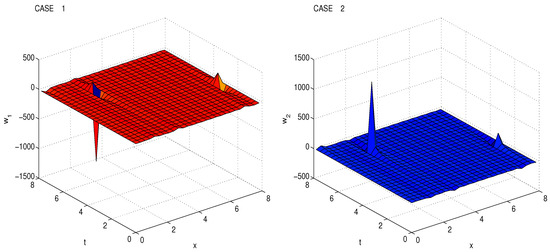
Figure 1.
Exact solutions of conformable mRLW equation Case 1 and Case 2 using , , , , , ,
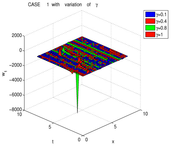
Figure 2.
Exact solutions of conformable mRLW equation (Case 1) using , , , , , , , , and .
4.2. Exact Solutions of Conformable Space-Time pKP Equation
The pKP equation is a universal integrable system in two spatial dimensions, which was first proposed by Vladimir l. Petviashvili (1936–1993) and Boris B. Kadomtsev (1928–1998). They explain water waves with a long wave length, especially water waves that have frequency dispersion and weak non-linear restoring forces.
Consider the conformable space-time pKP Equation [18] as:
where . Firstly, we apply the conformable derivative as:
Here the transformation is given in Equation (28) and the transformation variable is . The following conversions will be obtained from the transformation given in Equation (28):
Here p, m and l are constants and the transformation variable is . Then, we obtain the following ODE by putting Equation (29) in Equation (27):
Now we apply the division theorem to obtain the first integrals. As stated in FIM, it is supposed that X and Z are non-trivial solutions for the above system (c.f. Equation (31)). Hence, by the division theorem in , there exists an irreducible polynomial such that
where for . Now there exists in a polynomial such that
Here represent polynomials in X, it is implied by Equation (34) that polynomial is of a constant nature, so . For convenience, we consider . We inferred that can only be 0 or 1, by substituting values of and in Equations (35) and (36) and balancing the degrees of the functions and . Let us consider , therefore Equation (35) takes the following form:
where the integration constant is denoted by B.
After substituting the values of , in Equation (36) and equating all coefficients for some power of X, we get a nonlinear system of algebraic equations. Afterwards, we obtain different combinations of constants as given below:
Case 1: we have,
The first solution of the conformable pKP equation is attained (c.f. Equation (39) with Equation (31a)).
Case 2: We get,
The second solution of the conformable pKP equation is attained (c.f. Equation (42) with Equation (31a)).
The solutions are presented in Figure 3. In Figure 4 the solutions are presented for different values of .
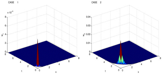
Figure 3.
Exact solutions of conformable pKP equation Case 1 and Case 2 using
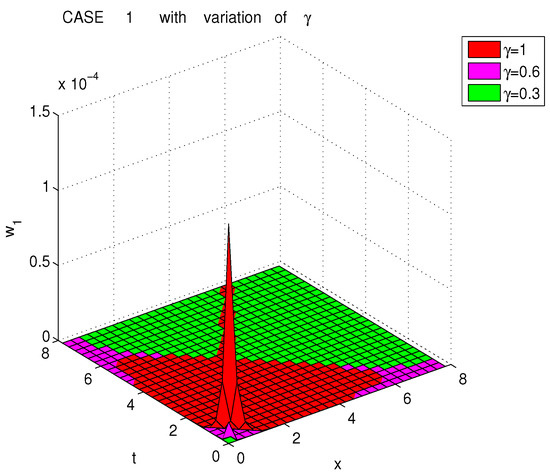
Figure 4.
Exact solutions of conformable pKP equation Case 1 using , , , and .
4.3. Exact Solutions of Conformable Space-Time DLW System
The Dispersive long wave system in two spatial directions is now discussed.
Consider the conformable space-time DLW system as [27,28]:
where represents the order of Equation (44) and .
Firstly, we apply the conformable derivative as:
where the transformation is given in Equation (45) and the transformation variable is . The following conversions will be obtained from the transformation given in Equation (45):
Here p, m and l are constants and the transformation variable is . Then, we obtain the following ODE by putting Equation (46) in Equation (44):
Now consider Equation (47a) and taking the integration constant as zero, we have:
Integrating Equation (47b) w.r.t and taking the integrating constant as zero we have:
Now we apply the division theorem to obtain the first integral. As stated in FIM, it is supposed that X and Z are non-trivial solutions for the above system (c.f. Equation (51)). Hence by the division theorem in there exists irreducible polynomial such that
where for . Now there exists in a polynomial such that
Here represent polynomials in X, it is implied by Equation (54) that polynomial is of a constant nature, so . For convenience, we consider . We inferred the can only be 0 or 1 by substituting values of and in Equations (55) and (56) and balancing the degrees of the functions and . Let us consider , therefore Equation (55) takes the form:
where the integration constant is denoted by .
After substituting the values of , in Equation (56) and equating all coefficients, for some power of X, we get a nonlinear system of algebraic equations. Afterwards, we obtain different combinations of constants as given below:
Case 1: we have,
The first solution of the conformable DLW system is attained (c.f. Equation (59) with Equation (51a)).
Case 2: we get,
The second solution of the conformable DLW system is attained (c.f. Equation (63) with Equation (51a)).
The solutions are presented in Figure 5. In Figure 6 the solutions are presented for different values of .
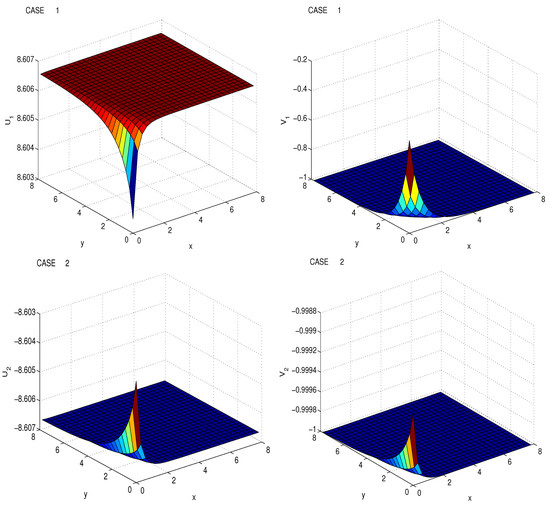
Figure 5.
Exact solutions of the conformable DLW equation Case 1 and Case 2 using
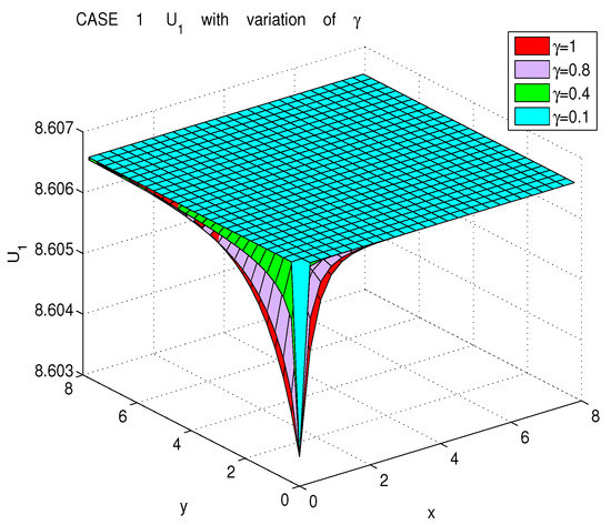
Figure 6.
Exact solutions of the conformable DLW equation (Case 1) using , , and .
5. Conclusions
In this paper, we presented the exact solutions of mathematical physics models. FIM was applied to attain the solutions of conformable mRLW, pKP and DLW systems. FIM was proved as an effective technique to construct new exact solutions of non-linear PDEs that appear in engineering, physics and biology.
Author Contributions
Conceptualization, S.J. and D.B.; methodology, S.R. and K.S.A.; software, S.J. and S.R.; validation, M.A. and A.H.; formal analysis, S.J. and S.R., writing—original draft preparation, S.J. and S.R.; writing—review and editing, K.S.A.; supervision, D.B.; project administration, M.A.; funding acquisition, M.A.
Acknowledgments
The authors extend their appreciation to the Deanship of Scientific Research at King Saud University for funding this work through research group no RG-1439-293.
Conflicts of Interest
The authors declare no conflict of interest.
References
- Kilbas, A.A.A.; Srivastava, H.M.; Trujillo, J.J. Theory and Applications of Fractional Differential Equations. North-Holland Mathematics Studies; Elsevier Science: Amsterdam, The Netherlands, 2004. [Google Scholar]
- Mille, K.S.; Ross, B. An Introduction to the Fractional Calculus and Fractional Differential Equations; Wiley: New York, NY, USA, 1993. [Google Scholar]
- Podlubny, I. Fractional Differential Equations: An Introduction to Fractional Derivatives, Fractional Differential Equations, to Methods of Their Solution and Some of Their Applications (Vol. 198); Elsevier: San Diego, CA, USA, 1999. [Google Scholar]
- Elizarraraz, D.; Verde-Star, L. Fractional divided differences and the solutions of differential equations of fractional order. Adv. Appl. Math. 2000, 24, 260–283. [Google Scholar] [CrossRef][Green Version]
- Levi, L.; Payroutet, F. A time-fractional step method for conservation lawrelated obstacle problems. Adv. Appl. Math. 2001, 27, 768–789. [Google Scholar] [CrossRef]
- Momani, S.; Odibat, Z. Homotopy perturbation method for nonlinear partial differential equations of fractional order. Phys. Lett. A 2007, 365, 345–350. [Google Scholar] [CrossRef]
- Dehghan, M.; Manafian, J.; Saadatmandi, A. Solving nonlinear fractional partial differential equations using the homotopy analysis method. Numer. Methods Partial Differ. Equ. 2010, 26, 448–479. [Google Scholar] [CrossRef]
- Xia, T.C.; Wang, L. New explicit and exact solutions for the Nizhnik-Novikov-Vesselov equation. Appl. Math. E-Notes 2001, 1, 139–142. [Google Scholar]
- Elwakil, A.S.; Abdou, M.A. New exact travelling wave solutions using modified extended tanh-function method. Chaos, Solitons Fractals 2007, 31, 840–852. [Google Scholar] [CrossRef]
- Fan, E. Extended tanh-function method and its applications to nonlinear equations. Phys. Lett. A 2000, 277, 212–218. [Google Scholar] [CrossRef]
- Aksoy, E.; Kaplan, M.; Bekir, A. Exponential rational function method for space-time fractional differential equations. Waves Random Complex Media 2016, 26, 142–151. [Google Scholar] [CrossRef]
- Zhang, S.; Zhang, H.Q. Fractional sub-equation method and its applications to nonlinear fractional PDEs. Phys. Lett. A 2011, 375, 1069–1073. [Google Scholar] [CrossRef]
- Feng, Z. On explicit exact solutions to the compound Burgers-KdV equation. Phys. Lett. A 2002, 293, 57–66. [Google Scholar] [CrossRef]
- Javeed, S.; Saif, S.; Waheed, A.; Baleanu, D. Exact solutions of fractional mBBM equation and coupled system of fractional Boussinesq-Burgers. Results Phys. 2018, 9, 1275–1281. [Google Scholar] [CrossRef]
- Javeed, S.; Saif, S.; Baleanu, D. New exact solutions of fractional Cahn–Allen equation and fractional DSW system. Adv. Differ. Equ. 2018, 1, 459. [Google Scholar] [CrossRef]
- Abdel-Salam, E.A.; Gumma, E.A. Analytical solution of nonlinear space–time fractional differential equations using the improved fractional Riccati expansion method. Ain Shams Eng. J. 2015, 6, 613–620. [Google Scholar] [CrossRef]
- Dehghan, M.; Salehi, R. The solitary wave solution of the two-dimensional regularized long-wave equation in fluids and plasma. Comput. Phys. Commun. 2011, 2, 305–320. [Google Scholar] [CrossRef]
- Aguero, M.; Najera, M.; Carrillo, M. Non classic solitonic structures in DNA’s vibrational dynamics. Int. J. Mod. Phys. B 2008, 22, 2571–2582. [Google Scholar] [CrossRef]
- Eslami, M. Solutions for space time fractional (2+1) dimensional dispersive long wave equations. Iran. J. Sci. Technol. Trans. A Sci. 2017, 41, 1027–1032. [Google Scholar] [CrossRef]
- Neirameh, A. New soliton solutions to the fractional perturbed nonlinear Schrodinger equation with power law nonlinearity. SeMA J. 2016, 73, 309–323. [Google Scholar] [CrossRef]
- Khalil, R.; Al-Horani, M.; Yousef, A.; Sababheh, M. A new definition of fractional derivative. J. Comput. Appl. Math. 2014, 264, 65–70. [Google Scholar] [CrossRef]
- Atangana, A.; Baleanu, D.; Alsaedi, A. New properties of conformable derivative. Open Math. 2015, 13, 889–898. [Google Scholar] [CrossRef]
- Abdeljawad, T. On conformable fractional calculus. J. Comput. App. Math. 2015, 279, 57–66. [Google Scholar] [CrossRef]
- Benkhettoua, N.; Hassania, S.; Torres, D.F.M. A conformable fractional calculus on arbitrary time scales. J. King Saud Univ. Sci. 2016, 28, 93–98. [Google Scholar] [CrossRef]
- Tasbozan, O.; Cenesiz, Y.; Kurt, A. New solutions for conformable fractional Boussinesq and combined Kdv-mKdv equations using the Jacobi elliptic function expansion method. Eur. Phys. J. Plus 2016, 131, 244. [Google Scholar] [CrossRef]
- Hammad, M.A.; Khalil, R. Conformable fractional heat equation. Int. J. Pure Appl. Math. 2014, 94, 215–221. [Google Scholar]
- Lou, S.Y. Painleve test for the integrable dispersive long wave equation in two space dimensions. Phys. Lett. A 1993, 176, 96–100. [Google Scholar] [CrossRef]
- Paguin, G.; Winternitz, P. Group theoretical analysis of dispersive long wave equations in two space dimensions. Phys. D Nonlinear Phenom. 1990, 46, 122–138. [Google Scholar] [CrossRef]
© 2019 by the authors. Licensee MDPI, Basel, Switzerland. This article is an open access article distributed under the terms and conditions of the Creative Commons Attribution (CC BY) license (http://creativecommons.org/licenses/by/4.0/).