Article

Kernel-Based Robust Bias-Correction Fuzzy Weighted C-Ordered-Means Clustering Algorithm

1
Colleage of Information Science and Engineering, Yanshan University, Qinhuangdao 066004, China
2
College of Mathematics and Information & Science Technology, Hebei Normal University of Science & Technology, Qinhuangdao 066004, China
*
Author to whom correspondence should be addressed.
Symmetry 2019, 11(6), 753; https://doi.org/10.3390/sym11060753
Submission received: 29 April 2019 / Revised: 21 May 2019 / Accepted: 30 May 2019 / Published: 3 June 2019

Abstract

:
The spatial constrained Fuzzy C-means clustering (FCM) is an effective algorithm for image segmentation. Its background information improves the insensitivity to noise to some extent. In addition, the membership degree of Euclidean distance is not suitable for revealing the non-Euclidean structure of input data, since it still lacks enough robustness to noise and outliers. In order to overcome the problem above, this paper proposes a new kernel-based algorithm based on the Kernel-induced Distance Measure, which we call it Kernel-based Robust Bias-correction Fuzzy Weighted C-ordered-means Clustering Algorithm (KBFWCM). In the construction of the objective function, KBFWCM algorithm comprehensively takes into account that the spatial constrained FCM clustering algorithm is insensitive to image noise and involves a highly intensive computation. Aiming at the insensitivity of spatial constrained FCM clustering algorithm to noise and its image detail processing, the KBFWCM algorithm proposes a comprehensive algorithm combining fuzzy local similarity measures (space and grayscale) and the typicality of data attributes. Aiming at the poor robustness of the original algorithm to noise and outliers and its highly intensive computation, a Kernel-based clustering method that includes a class of robust non-Euclidean distance measures is proposed in this paper. The experimental results show that the KBFWCM algorithm has a stronger denoising and robust effect on noise image.

1. Introduction

Clustering analysis is a significant technique in data analysis, which covers a wide range of applications in many areas such as data mining [1,2], image processing [3,4,5], computer vision [6] and artificial intelligence [7,8]. Generally, the clustering methods can be divided into four types, namely hierarchical clustering, graph theory, Density-based clustering and minimization objective function [9]. In this paper, we will focus on the fuzzy clustering method by minimizing the objective fuzzy function and apply it to image segmentation. Image Segmentation is a image processing technique, dividing the image into several specific non-overlapping regions with unique characteristics and proposing objectives of interest. It is a crucial step from image processing to image analysis. The existing segmentation methods mainly consist of the following categories: threshold-based segmentation, region-based segmentation, edge-based segmentation, specific theory-based segmentation and so forth. Specifically speaking, these methods contain clustering [10,11], region growing [12], watershed transformation [13], active contour model [14], meanShift [15], graph Cut [16], spectral clustering [17], Markov random field [18], Neural network [19] and so forth. The image segmentation process is also a marking process, in which pixels belonging to the same area are given the same number. Image segmentation has always been one of the most challenging tasks in image processing and computer vision [20,21]. Nowadays, there have been many types of methods for image segmentation [22,23,24,25], however, these methods are all not robust and effective enough for a large number of different images.

1.1. The Introduction of Fuzzy Clustering

How to segment a given image? And how to segment it in a rational way? These are the major problems needing to be solved by the clustering algorithm. The solution to such problems: under the same measure condition, the data in classes are made, as much as possible, to have the minimum sum of distances within classes and have the maximum sum of distances between classes. Dunn [26,27,28] is the first one who successively introduced the fuzzy set proposed by Zadeh [29] into the clustering analysis [30]. He subsequently proposed the Fuzzy C-means Clustering algorithm (FCM), which was later popularized by Bezdek [31,32,33,34,35,36,37]. Nikhil and Bezdek [38] conducted some studies on the effectiveness of FCM clustering in the early days, providing an introduction of a subtle but important parameter, that is, m the weighted index of FCM model. This algorithm has been the most famous fuzzy clustering algorithm, a combination of clustering analysis and fuzzy theory. The introduction of fuzziness makes each image pixel have a sense of belonging. Compared with the hard segmentation method, this fuzzy clustering method preserves more information in the original image, thus making the processed image clearer.
Fuzzy clustering is an unsupervised machine learning algorithm, which can be divided by constantly modifying the clustering center and membership matrix. Fuzzy clustering is used to partition a set of given observed input data vectors or image pixels into c-clusters so that members of the same cluster are similar to one another and members of different clusters are dissimilar from one another. Of which, C the number of clusters is usually predefined or set by some criteria of validity or prior knowledge. So far, the fuzzy clustering has been widely studied and applied into various fields [39,40,41,42,43]. The FCM algorithm introduces the fuzziness into the attributes of each sample and each sample is assigned a membership degree between zero and one. The objective function of the classical FCM algorithm is defined by the membership degree of the sample to the clustering center and the Euclidean distance. FCM algorithm is sensitive to noise due to its restricted condition. Thus, local spatial information is necessarily introduced into the objective function to improve the robustness of the FCM algorithm for image segmentation.
Since Bezdek’s masterpiece came out, many researchers have improved the performance of the classical FCM algorithm from different perspectives and approaches. It will be discussed from the following three aspects: (1) By introducing the fuzzy mean clustering of spatial information, the local spatial information is introduced into the objective function for calculation; (2) The sequence mean value and fuzzy mean clustering algorithm are introduced to combine the fuzzy C-means clustering with robust ordered statistics, by updating their typicalities and reordering data items in each iteration of the clustering process. The data closer to the cluster center are of high typicality, while those farther from the cluster center low typicality. Thus, outliers and noisy data items are classified as low typicality without damaging the clustering process; (3) In order to overcome the problem that the distance between one point and two prototypes is equal in the FCM, Krishnapuram and Keller [43,44] proposed a new clustering model called Possibilistic C-Means (PCM). On this basis, two new models were proposed in succession, respectively called Fuzzy Possibilistic C-Means (FPCM) [45] and Possibilistic Fuzzy C-Means (PFCM) [46]. The algorithm proposed in this paper is integrated with the first two aspects (1) and (2), that is, this algorithm will combine the spatial information and typicality of the data, with an aim to ensure the insensitivity to noise and preservation of image details.

1.2. Introduction to FCM Clustering with Local Spatial Information

The traditional Hard C-means (HCM) Clustering Algorithm is very simple (the membership degree is either 0 or 1) [47], resulting in poor image segmentation. While FCM is more tolerant of ambiguity and retain more original image information. In addition, it is effective for images with simple texture and background, therefore, FCM is better than HCM. The FCM algorithm performs well in segmentation of most noiseless images, however, it shows unsatisfactory performance in segmentation of images with complicated texture and background that are corrupted by noise, outliers and artifacts in the other image processes. For instance, the intensity inhomogeneity caused by radiofrequency (RF) coils in magnetic resonance imaging (MRI) is because this algorithm only takes into account the grayscale information without considering the spatial information and because it cannot avoid the noise interference. In order to solve the problems mentioned above, many scholars have proposed to introduce local spatial information into the objective function. For instance, Tolias [48] proposed to add spatial information to membership degree. Ahmed [49] (2002) and Pham [50] (2001) proposed a bias correction fuzzy c-means (FCM) algorithm, which introduces the spatial context information of images, adds neighborhood pixel information to the objective function of the FCM algorithm as a penalty term and attempts to make neighborhood pixels and central pixels produce more consistent clustering results in the segmentation process. Liew [51] used a new neighborhood weighted dissimilarity measure for the Euclidean distance in the FCM objective function. Compared with FCM, this algorithm uses more spatial information, which can better realize the clustering and segmentation of image data. Chuang et al. [52] proposed the spatial information problem in image segmentation earlier. They believe that the consideration of spatial information can bring the following benefits: “(1) it yields regions more homogeneous than those of other methods, (2) it reduces the spurious blobs, (3) it removes noisy spots and (4) it is less sensitive to noise than other techniques”. This wonderful idea has influenced many scholars and made them consider more the spatial factors of image segmentation. Chen and Zhang [53] proposed two variants of FCMS1 and FCMS2, respectively using the FCM clustering algorithm based on pre-acquired mean filtering and that based on median filtering to affect the marking of image pixels, instead of updating the marking of all image pixels in each iteration.
In order to achieve a better implementation of the FCM clustering algorithm, Szilagyi [54] introduced a new factor, starting from the standard FCM and its bias-correction version, thus reducing the amount of computation required and offering a fast way to segment high quality brain images. An enhanced fuzzy C-means clustering (EnFCM) algorithm was proposed based on grayscale rather than image pixel with an aim to improve the running speed of FCMS. However, when constructing the linear weighted sum image, the EnFCM algorithm lacks the spatial information, causing that the image segmentation results are sensitive to salt and pepper noise. In order to improve the segmentation results of EnFCM, Cai et al. [55] proposed a fast generalized FCM algorithm (FGFCM), which first redefines the linear weighted sum images by utilizing grayscale and spatial information of each pixel’s neighborhood window of the original image and then performs clustering on its gray histogram. This algorithm introduces a new factor as a local (space and grayscale) similarity measure, which is aimed to ensure the noise immunity and detail retention of image segmentation. Meanwhile, the empirical adjustment parameter α required in EnFCM is removed and finally a grayscale histogram is clustered. However, there is still a parameter needing to be experimentally determined. The FGFCM algorithm further improves the balance between noise and detail, enhances the robustness of the algorithm to noise and improves the computational efficiency of FCM to some extent. However, it requires more parameters than EnFCM. The contribution strength of the spatial neighborhood information of FGFCM algorithm is hard to control and needs to be set manually. In addition, the strength value is a global variable and the distribution of noise cannot be fully considered. Hathaway et al. [56] first proposed a generalized fuzzy C-means clustering algorithm (GFCM) and on this basis subsequently proposed a new generalized fuzzy C-means clustering algorithm (GIPF_FCM) [57] to accelerate the convergence speed of the FCM clustering algorithm.
Later, with the rise of kernel technology [58,59], Zhao et al. [60] put forward kernel-based version of GIFPFCM with spatial constraint (KGFCMS1 and KGFCMS2) to improve the cluster performance. Yang et al. [61] proposed a Gaussian kernel-based FCM (GKFCM) algorithm and introduced a class of robust non-euclidean distance measures to derive a new objective function. It is a generalization of FCM, BCFCM, KFCMS1 and KFCMS2 algorithms, having more efficiency and robustness to noise and outliers.
Wang et al. [62] proposed local and non-local FCM clustering algorithm to reduce the influence of noise in the process of image segmentation. By using a new dissimilarity index to replace the usual distance measures, this method incorporates local spatial context and non-local information into the standard FCM clustering algorithm, where the image local information takes into account the weighted distance between the pixel and the class center.
Krinidis and Chatzis [63] proposed a robust fuzzy local information C-means clustering algorithm (FLICM) to ensure the insensitivity of noise and preservation of image details and to fuse the local spatial information with grayscale information using a new fuzzy method. Compared with the traditional FCM algorithm, this algorithm can utilize the spatial information and grayscale information, greatly improving the segmentation effect for images with noise. It replaces parameters used in the EnFCM with a new fuzzy factor, which can be translated into an objective function that ensure the noise immunity and image detail preservation.
FLICM overcomes the problem of parameter selection and improves image segmentation performance but it is not robust enough for local information of different images and fixed spatial distance. Meanwhile, FLICM uses variance information in the pixel neighbourhood to modify the fuzzy weight factors, thus improving the robustness and noise immunity of this algorithm. However, the image denoising effect is still poor for weak contrast images. In order to further improve the segmentation performance of FLICM, Gong et al. [64] proposed a kernel weighted fuzzy local information C-means algorithm (KWFLICM). This algorithm replaces the Euclidean distance measures in the FLICM algorithm with the nuclear distance measures and proposes a new local information weighted fuzzy factor. This fuzzy factor links the local spatial information with grayscale information and uses pixel neighborhood variance information to modify its fuzzy weighted factor to adaptively control the local spatial relationship, in order to enhance the robustness of FLICM to noise and outliers. However, KWFLICM has a higher computational complexity than FLICM.
Ahmed et al. [65] proposed an adaptively regularized kernel-based FCM framework (ARKFCM), aiming at the segmentation of brain magnetic resonance image. This algorithm utilizes the heterogeneity of neighborhood grayscale to obtain the local context information and replaces the Standard Euclidean distance with the Gaussian radial basis kernel functions. In this way, the robustness of preserving the image details is improved, the independence of cluster parameters is enhanced and the computing costs are reduced. Lei T et al. [66] proposed an improved FCM algorithm based on Morphological reconstruction and membership filtering (FRFCM), which is faster and more robust than FCM algorithm. By introducing morphological reconstruction operation, the local spatial information is incorporated into the FRFCM algorithm to ensure the anti-noise ability and image detail preservation.
Saranathan [67] introduced the non-local spatial information into the objective function by using variant parameters adaptive to the noise level of each pixel of the image, which has been extended to FCM to overcome the parameter selection to improve the robustness to noise. The FGFCM algorithm and the FLICM algorithm both use coordinate information to add spatial distance information to the clustering process. Zhao et al. [68] believe that the Euclidean distance cannot reflect the spatial information of the image well. Therefore, they proposed a neighborhood weighted fuzzy C-means (NWFCM) clustering algorithm, namely Neighborhood Weight (NW) distance to reduce the running time of FLICM and KWFLICM and strengthen the robustness of the algorithm to noise. Although NWFCM uses more parameters, NWFCM is faster than FLICM and KWFLICM because image filtering is performed before the iteration begins. However, the NWFCM algorithm is still time-consuming due to the calculation of the NW distance and the parameter selection. Guo et al. [69] proposed an adaptive Noise Detection-based FCM(NDFCM). This algorithm overcomes the above mentioned shortcoming, in which the trade-off parameters are automatically adjusted by measuring the local variance of the gray scale.

1.3. Introduction of Clustering Algorithm Based on Ordered Means

The fuzzy c-ordered-means clustering algorithm (FCOM) proposed by Jacek M. [70] integrates the FCM clustering with the robust order statistics put forward by Huber [71] and applies the Ordered Weighted Averaging (OWA) proposed by Yager [72] to fuzzy clustering, thus significantly improving its robustness. This algorithm calculates the typicality of each data item instead of assigning weights to attributes. The data item is sorted and their typicality is updated in each iteration of the clustering process. The data closer to the cluster center are of high typicality, while those farther from the cluster center low typicality. Thus, outliers and noisy data items are classified as low typicality without damaging the clustering process. Therefore, this method has better performance in terms of noise and outlier data.
On the basis of FCOM, a new clustering algorithm was put forward called Fuzzy weighted C-ordered means clustering algorithm (FWCOM) [73]. This algorithm searches clusterers in the fuzzy Subspace of the original task space and assigns weights to the dimensions (attributes) in each cluster. The weight is the number from the unit interval (0,1). In order to enhance the robustness of the algorithm to outliers and noise, it is combined with sorting techniques.
For the above-mentioned algorithm, this paper proposes an adaptive filtering based fuzzy clustering algorithm by combining the FWCOM clustering algorithm with the FCM clustering algorithm with spatial information. This algorithm first determines the non-local parameter balance factor according to the strength of the local spatial information, meanwhile calculating the typicality of each data item, sorting the data items and updating their typicalities in each iteration of the clustering process, with an aim to more accurately reflect the spatial structure information contained in the image. Then it uses this balance factor to make an effective combination of the filtered image and the median filtered image of the original image. The obtained adaptive filtered image adaptively determines the degree of filtering according to the noise intensity, thus improving the algorithm’s ability to suppress noise and the robustness of the algorithm.

1.4. Introduction of Fuzzy Clustering Based on Kernel Method

Kernel method [74,75,76,77,78,79], as one of the most studied subjects in machine learning field, has been widely applied in pattern recognition and function approximation. This method is a kind of algorithms for pattern recognition and its most famous uses are in the support vector machine (SVM) [75,76,77], Kernel Fisher’s Linear Discriminant Analysis (KFLDA) [78], Kernel Principal Component Analysis (KPCA) [79] and Kernel Perceptron algorithm [80]. Kernel tricks are powerful. The kernel function is preferred, since it provides a connection from linear to non-linear through some non-linear mapping, transforming into higher (possibly infinite) dimensional feature space from the original low dimensional inner product input space, while not explicitly mapping the input points to this space. The usual expression for kernel function representing the inner product in the feature space is as shown below:
K x , y = Φ x , Φ y
According to pattern recognition theory, the linearly inseparable pattern in low dimensional space can be linearly separable by non-linear mapping to high-dimensional feature space. However, if this technique is directly used for classification or regression in the high dimensional space, there will be some problems such as determination of the form and parameters, as well as the feature space dimension of non-linear mapping function. The biggest obstacle is the exponential growth of computation time, that is, there exits the ”dimensional curse” in high dimension feature space computation. The use of kernel function can effectively solve the problems above. However, this algorithm can merely represented by the inner product between two vectors, therefore, there is no need to calculate the mapping. All we need to do is to replace this inner product with some other suitable space. In this process, there is more likelihood that the complex non-linear issues in the original low dimension space can be linearly processed and solved in the transformed space. This is highly desirable.
It can be concluded that the kernel function has the following properties:
(1)
The introduction of kernel function avoids the ”dimensional curse” and significantly reduces the computation. It is a perfect trick to shift the ”disaster” effect from the low dimension of the input space to the processing of high-dimensional vector product, thus reducing the computation.
(2)
There is no need to know the form and parameters of the non-linear mapping function.
(3)
The kernel function method can select different kernel functions and algorithms according to different applications and combine them together to form a variety of different kernel function-based techniques, while the design of kernel functions and algorithms can be performed separately.
(4)
The kernel function implicitly turns the originally complicated computation into a mapping computation and changes the initial form and parameters of computation into the mapping from input space to feature space and thus having an effect on the properties of feature space, finally achieving the purpose of computation.
Therefore, the inner product form of FCM [81,82] guides us to apply the kernel method to clusters of complex data. However, one major difference of the proposed method in this paper from the method proposed in [81,82] lies in that we directly convert the all centroids in the original space together with the given data sample into a high dimension feature space with (implicit) mapping, instead of using so-called double representations for each centroid, that is, a linear combination of all given dataset (samples). The direct conversion brings about the following benefits:
(1)
By using robust kernel, a class of robust non-euclidean distance measure is introduced. A new class of robust non-euclidean distance measure is introduced into the input space and then the robust second-order metric (kernel) is used to replace the non-robust Euclidean distance metric. Thus, data clustering or image segmentation can be carried out more effectively.
(2)
Maintain the computational simplicity of FCM.
(3)
It is more likely to reveal the inherent non-euclidean structure of the data.
(4)
The clustering results can be intuitively explained.
(5)
Data sets with missing values are easily handled [83].
Compared with the non-kernel replacement algorithm, this algorithm is more robust to noise and outliers in image segmentation, especially under the spatial constraints.

1.5. Theoretical Classical FCM Algorithm and Its Relationship with KBFWCM Algorithm

The Table 1 tabulates the key papers on the evolution of FCM, which are mentioned in the introduction. This table shows the evolution of FCM and the contribution that different scholars have made to its development in each stage. The Diagram-1 shows that the algorithm proposed in this paper is an integration of previous work. KBFWCM algorithm integrates three ideas. In the Figure 1, the first line is about the evolution of fuzzy kernel, the second line is about the evolution of FCM algorithm considering spatial factors and the third one is about the consideration of typicality of fuzzy clustering. This paper integrates these three ideas into a whole. It can be seen that the proposed algorithm is better than other algorithms in the following three aspects: (1) The algorithm is a combination of three popular algorithms, which combines the kernel algorithm and takes into account the spatial factors around pixels and typicality of data itself; (2) The introduction of kernel algorithm reduces the computation of this proposed algorithm; (3) The spatial factors and the typicality of data itself make the algorithm insensitive to outliers and ambiguity points.

1.6. Structure of the Paper

The rest of this paper is organized as follows:
The second chapter offers an introduction to the basic knowledge and calculation process of the KBFWCOM algorithm. In the third chapter, we first replace the Euclidean norm of the objective function with the kernel-induced non-euclidean distance measure and subsequently minimize these new objective functions to obtain a group of kernel fuzzy clustering algorithms with spatial constraints. The fourth chapter provides a comparison of experimental results. The fifth chapter gives the conclusion.

2. Related Work

A robust algorithm is supposed to have the following properties: (1) there should be fairly good precision in the assumed model; (2) small deviations from model assumptions should only cause damage to a small amount of performance; (3) relatively large deviations from model assumptions should not cause disaster. This paper will introduce the BFWCOM algorithm combining spatial information and fuzzy weight.

2.1. Criterion Function for BFWCOM Algorithm

The objective function J U , V can be minimized in a manner similar to the standard FCM algorithm. The BFWCOM’s criterion function takes the following form:
J U , V = i = 1 c k = 1 n β i k u i k m x k v i 2 + α N R u i k m r N i x r v i 2
The application area of its criterion function:
J g f c = U c N u i k [ 0 , 1 ] ; i = 1 c β i k u i k = f k ; 0 < k = 1 N u i k < N

2.2. Clustering Prototype and Bias Field Update

According to the reference [49], a bias field component η r is introduced into the objective function J U , V . These three conditions will be derived in the following sections.
J m U , V = i = 1 c k = 1 n β i k u i k m D i k + α N R u i k m γ i
where: D i k = y k η k v i 2 , γ i = r N i y r η r v i 2 .

2.3. Calculation of Typicality of Data

Spatial neighborhood Information is of great significance for image segmentation. However, the execution of a large number of clustering algorithms is based on the clustering of Gray Histogram rather than summing the image pixels. The number of grayscale levels in an image is usually much smaller than that of pixels and the calculation time is very short. However, only the neighborhood grayscale value information is added to the clustering process, while the distance information of the spatial neighborhood points is not taken into account. The effect of all neighborhood points on the central point is the same, which is obviously not in line with the actual situation. The neighborhood points that are closer to the central point should have more effect on the central point, while the neighborhood points that are farther away from the central point should have less effect on it. Based on this reason, the typicality of data is calculated.
Here we should first discuss the ordering of data items. For each data item in each cluster, the properties of each attribute are computed separately. To do this, the data items are sorted by their distance from the cluster center. The d-th attribute of the closest data item is marked with the ordinal number 1, while that of the farthest data item n (n stands for the number of data items). The value β c k d represents the characteristic of the d-th attribute relative to the k-th data item of the c-th cluster and is calculated with the function:
β c k d = p c n χ c k d 2 p l n + 1 2 1 0
It is called piecewise linear ordered weighted averaging (PLOWA) or
β c k d = 1 1 + exp 2.944 p a n χ c k d p c n
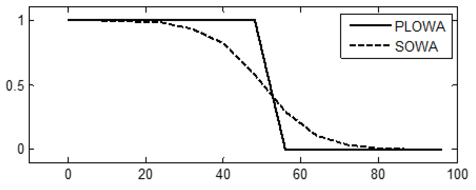
Among them, ∧ and ∨ respectively represents the minimum and maximum operations. These two functions, which can be called weighting functions, are not increased relative to the parameter χ c k d { 1 , 2 , , n } . For χ c k d = p c n , both functions are equal to 0.5. Parameters p l > 0 and p a > 0 affect the slope. In the case of a piecewise linear function, for χ c k d [ p c n p l n , p c n + p l n ] , its value is linearly reduced from 1 to 0 (see Figure 2 for details). In the case of the S-function, for χ c k d [ p c n p a n , p c n + p a n ] , its value dropped from 0.95 to 0.05. The functions defined by the formula (4) and the formula (5) are respectively called S-ordered weighted average (SOWA) and piecewise linear ordered weighted averaging (PLOWA) in the rest of the work. If residual ordering is not applied, this is equivalent to using a uniform weighting function based on OWA-UOWA for all χ c k d , β c k d = 1 . Then we call this case an unordered cluster (or no weighting function).
It is called S-ordered weighted average (SOWA) [71]. In these two functions, represents the k-th data item index after reordering the distance relative to the c-th cluster of the d-th attribute. The two functions are shown in Figure 1, n = 100 and p a = 0.2 , p c = 0.5 , p l = 0.2 .
The importance of this data item affects the central location of the cluster. The global characteristic f k of the k-th data item is calculated using s-norm (⬨) of all cluster data item characteristics:
f i = β 1 i β 2 i β c i
We use the largest operator as the s-norm operator.

3. Kernel-Induced Robust Bias Correction Fuzzy Weighted C-Order Mean Clustering Algorithm

Considering the still relatively large computation of BFWCOM algorithm, the computational efficiency of the algorithm should be improved and the kernel method is one of the best methods.

3.1. Definition and Theorem of Kernel Function

With respect to the fuzzy kernel function clustering algorithm, some definitions and theorems related to kernel function are applied, mainly including the knowledge as shown in the following sections [84,85].

3.1.1. Definition of Kernel Function

1
Definiton of feature space: Suppose the pattern x p maps the input space p to a new space by mapping Φ , that is, Φ : x χ p Φ ( x ) F H ( p H ) . Then, F is called the feature space.
2
Definition of kernel function: Let X be a non-empty set, H be a inner product space, Φ be the mapping from X to H, if the function K : X × X R satisfies the condition: for x , y X , K x , y = Φ x , Φ y . Then, K is the kernel function.
3
Definition of positive semi-definite kernel function: if the continuous symmetric function K x , y L X × Y satisfies the following formula:
X × Y K x , y f x f y d x d y 0 , f L 2 X
Then, the function K x , y is a positive semi-definite kernel function. In the discrete case, for any positive integer n, sample set x 1 , x 2 , , x N p and constant a 1 , a 2 , , a N , if the symmetric function K x , y L X × Y and satisfies the following formula:
i , j = 1 n a i a j K x i , x j 0
Then, K x , y is a positive semi-definite kernel function.
4
Definition of Mercer conditions: The necessary and sufficient condition for any symmetric function K x , y that can be represented as the inner product form K x , y = Φ x , Φ y is positive semi-definite, that is,
X × Y K x , y f x f y 0
For the discrete case, the following matrix
K x 1 , x 1 K x 1 , x 2 K x 1 , x n K x 2 , x 1 K x 2 , x 2 K x 2 , x n K x n , x 1 K x n , x 2 K x n , x n
is a positive semi-definite matrix for all x 1 , x 2 , , x N .
The nonnegative condition is as follows:
X × Y K x , y f x f y 0 , f L 2 x
corresponds to the positive semi-definite condition in finite case.

3.1.2. The Fundamentals of Kernel Functions

The following theorem can be derived from definitions 3 and 4.
Mercer’s theorem: The so-called positive semi-definite function K x i , x j means to have the training data set x 1 , x 2 , , x N . Let’s define a matrix element K x i , x j , for this matrix n * n , if this matrix is positive semi-definite, then K x i , x j is called a positive semi-definite function. This mercer theorem is not a necessary condition for kernel functions. It is only a sufficient condition, that is, the functions that do not satisfy the mercer’s theorem can also be kernel functions.
Mercer’s theorem shows that in order to prove that K is an effective kernel function, we just need to find each K i j in the training set and then determine whether the matrix K is positive semi-definite or not (The principal minor in the upper left corner is greater than or equal to zero) instead of looking for Φ .
The fundamental principle of the kernel method: According to definitions (1) and (2), in the case where the sample set is non-linearly separable, a non-linear transformation formula is used to map the data in the input mode space R to the high-dimensional feature space F, namely, R F , in which a new classification function is constructed in the F. Thus, the new classification function can be linearly separable in high dimensional space. It is worth noting that we only need to replace the inner product operation with kernel function K x , y = Φ x Φ y , without the need to have the exact knowledge of the specific way of non-linear transformation.
In general, the transformation function Φ x is more complicated than kernel function K x , y , that is to say, the simple kernel function often corresponds to the complex mapping. As long as the kernel function that satisfies the Mercer condition, the computation of non-linear transformation can be greatly reduced. According to the fundamental principle of kernel function method, the design of new kernel method has two major problems as follows: (1) How to select and design kernel function, as well as to optimize related parameters in the kernel function; (2) What kind of learning algorithm is adopted to improve the learning algorithm? Different learning algorithms can construct different kernel methods, for instance, the introduction of kernel function into the clustering method can form kernel clustering method.

3.1.3. Gaussian Radial Basis Function Clustering Algorithm

The typical Gaussian radial basis kernel function (GRBF) are given below:
K ( x , y ) = exp x y 2 x y 2 σ 2 σ 2 = exp i = 1 p x i y i 2 / σ 2
where p is the dimension of the vector x. Obviously, for all x and the above mention GRBF kernel, K x , x = 1 .
As we all know, the parameter σ of Gaussian kernel function can affect the final results of kernel methods in some degree. In this paper, the sample variance is adopted to estimate σ 2 [61]. It is defined as
σ 2 = 1 n j = 1 n x j x ¯ 2 , x ¯ = 1 n j = 1 n x j
σ is the hyperparameter of the GRBF kernel and defines the characteristic length-scale of similarity among learning samples, that is, the proportion of the distance between samples before and after the feature space mapping from the perspective of weight space [86].
According the above mentioned kernel function method and Mercer theorem, in the feature space F, we can use the kernel function to replace the transformation function and use the non-linear transformation to map the sample set to the high-dimensional space F, thus improving the classification ability of the algorithm.

3.2. The Kernel-Induced Distance Based FCM (KFCM)

In literature [87], the Euclidean distance x k v i in the FCM clustering is rewritten as Φ x k Φ v i , where Φ · is a non-linear transformation function. According to the above, the objective function of the FCM clustering algorithm can be rewritten as below:
J m Φ = i = 1 c k = 1 N u i k m Φ ( x k ) Φ ( v i ) 2
Now by the kernel replacement, there is:
Φ ( x k ) Φ ( v i ) 2 = Φ ( x k ) Φ ( v i ) T Φ ( x k ) Φ ( v i ) = Φ ( x k ) T Φ ( x k ) Φ ( v i ) T Φ ( x k ) Φ ( x k ) T Φ ( v i ) + Φ ( v i ) T Φ ( v i ) = K ( x k , x k ) + K ( v i , v i ) 2 K ( x k , v i )
The square norm of a new class of feature space in the original data space can be obtained from the formula above. It can obviously seen that different kernel algorithms will produce different non-euclidean distance measures for the original space, thus forming a new clustering algorithm family. In particular, if the kernel function K x , y is taken as GRBF of (7), then (10) can be simplified to 2 1 K x k , v i . In addition, in order to facilitate the operation and robustness below, the Gaussian radial basis function (GRBF) kernel in (7) is applied ( In fact, the measurement based on (7) is robust through Huber’s robust statistics [71,88]). The parameter σ in (7) can be calculated through (8), then (9) can be rewritten as below:
J m Φ = 2 i = 1 c k = 1 N u i k m 1 K ( x k , v i ) .
J m Φ can be minimized under the constraint ( i = 1 c u i k m = 1 ) of the same U in FCM. Specifically speaking, if we use their first derivatives for u i k and v i respectively and set them to zero, then two necessary but insufficient conditions for J m Φ to be at the local minimum are obtained.
The clustering criterion of J m Φ the algorithm is to take the minimum value of, therefore, let the partial derivative of the objective function with respect to u i k and Φ v i be zero, the following two formula can be obtained:
u i k = 1 K ( x k , v i ) 1 ( m 1 ) j = 1 c 1 K ( x k , x j ) 1 ( m 1 )
v i = k = 1 n u i k m K ( x k , v i ) x k k = 1 n u i k m K ( x k , v i )
Obviously, the obtained center of mass or prototype v i is still in the original space rather than in the high-dimensional feature space. Thus, the simplicity of computation is still retained.
The procedure of KFCM clustering algorithm is described in Algorithm 1.
Algorithm 1 Kernel-based fuzzy c-means algorithm.
Input: Input dataset X = { x i } i = 1 N , the number of clusters c ( 2 c n ) , the threshold ε , the maximum number of iterations t,
 the fuzziness index m;
Output: c clusters of X,U,V.
 Begin
 Fix c , t m a x , m > 1 , ε > 0 , for some positive constant;
 Initialize the memberships μ k i 0 ;
 For t = 1 , 2 , , t max do:
  Update all prototypes ν k i t with Equation (13);
  Update all memberships μ k i t with Equation (12);
   Compute E t = max k i μ k i t μ k i t 1 ,
   If E t > ε , then t t + 1 and goto Step 4 else stop
   If t t m a x , then stop
  end for;
 return c clusters of X,U,V;
 end

3.3. Kernel-Induced Distance Based KBFWCM with Dpatial Constraints

In this section, the corresponding kernel version of KBFWCM algorithm will be constructed. Similar to the derivation of KFCM, we will kernelize the criterion (1) and adopt the GRBF kernel, that is, the replacement of a new distance-induced measure can help obtain the following new objective function:
J S m Φ = i = 1 c k = 1 N β i k u i k m D i k Φ + α N R i = 1 c k = 1 N u i k m γ i r Φ
where: D i k Φ = Φ y k η k Φ v i 2 , γ i r Φ = r N k Φ y ¯ r η r Φ v i 2 .
Available from the same calculation as (10):
J S m Φ = i = 1 c k = 1 N β i k u i k m D i r K + α N R i = 1 c k = 1 N u i k m γ i r K
where: D i r K = 1 K ( y k η k , v i ) , γ i r K = r N k 1 K ( y ¯ r η r , v i ) .
Of which, K x , y is still seen as GRBF. N R is the cardinality of u k i , y ¯ r η r represents the average data of neighborhood deviation of x k , N k is the neighbor set in the window around x k , α is the parameter to control the effect of the neighbor term, the relative importance of the adjustment term is inversely proportional to the Signal-Noise Ratio (SNR). The lower SNR requires higher parameter values.
The application of region which the criterion function of KBFWCM is faced with is (2).
The Laplace algorithm used to give the specific formula as follows:
G S m Φ = i = 1 c k = 1 N β i k u i k m D i r K + α N R i = 1 c k = 1 N u i k m γ i r K λ i = 1 c β i k u i k f k
Take the partial derivative of formula (16) with respect to u i k :
G S m Φ u i k = m β i k u i k m 1 D i r K + m α N R u i k m 1 γ i r K λ β i k = 0
λ m = u i k m 1 β i k D i r K + α N R γ i r K / β i k
The membership degree u i k is derived:
u i k = λ m 1 m 1 β i k D i r K + α N R γ i r K / β i k 1 1 m
Available from formula (2):
k = 1 c β k i u k i = f i
Substitute formula (19) into formula (20):
i = 1 c β i k u i k = i = 1 c β i k λ m 1 m 1 β i k D i r K + α N R γ i r K / β i k 1 1 m = f k
Derived from (21):
λ m 1 m 1 = f k i = 1 c β i k D i r K + α N R γ i r K α N R γ i r K β i k β i k 1 1 m 1
The membership formula obtained by substituting (22) into (19) is as follows:
u i k = f k β i k 1 K ( y k η k , v i ) + α N R β i k 1 r N i 1 K ( y ¯ r η r , v i ) 1 1 m i = 1 c β i k 1 K ( y k η k , v i ) + α N R β i k 1 r N i 1 K ( y ¯ r η r , v i ) 1 1 m
where: y ¯ r is the mean value of the bias field in the neighborhood of the pixel point x k .
The following can be obtained by derivative of the formula (16) with respect to v i :
v i = k = 1 N β i k u i k m K y k η k , v i y k η k + α N R r N k K ( y ¯ r η r , v i ) y ¯ r η r k = 1 N β i k u i k m K y k η k , v i + α N R r N k K ( y ¯ r η r , v i )
The following can be obtained by derivative of the formula (16) with respect to η k :
η k = k = 1 N β i k u i k m K y k η k , v i y k η k k = 1 N β i k u i k m K y k η k , v i
According to Huber’s robust statistics [71,88], KBFWCM obtained from (16), namely (23)–(25), is robust to noise and outliers. This feature can also provides the intuitive explanation from (16), that is, the data point x k is given an extra weight K ( y k η k , v i ) , which measures the similarity between x k and v i and when x k is an outlier ( x k is far away from other data points), K ( y k η k , v i ) will be very small. Therefore, the weighted sum of data points should be suppressed to generate robustness. The procedure of KBFWCM clustering algorithm is described in Algorithm 2.
Algorithm 2 KBFWCM algorithm.
Input: Input Image X = { x i } i = 1 N , the number of clusters c ( 2 c N ) , the threshold ε , the fuzziness index m, the parameter α ,
 the parameter β , the window size w;
Output: c clusters of X,U,V.
1:Begin
2:Fix X = { x i } i = 1 N , C 1 < c < N , m ( 1 , ) , ε > 0 ;
3:Initialize the center V [ 0 ] R p c ;
4:Initialize U with random numbers and normalize with constraint (2);
5:Initialize all β s with 1 s ;
6:Compute the mean or median filtered image X ¯ and set the iterative index k = 1;
7:For t = 1 to N do:
8:  Update the U [ t ] with (23) and constraint (2);
9:  for c = 1 to C do: (for each cluster);
10:   For d = 1 to p do: (for each attribute)
11:    for k = 1 to n do: (for each data item)
12:      e c d k : = | x k d v c d | (calculate the residual)
13:    end for (for each data item)
14:    sort residual; mark each residual with the number of sequences χ in the ordered sequence;
15:    for k = 1 to n do: (for each residual);
16:     calculate the characteristics of β c k d using formulas (4) and (5) or uniform weighting
17:    end for; (for each residual)
18:   end for; (for each attribute)
19:   Update the prototypes for t-th iteration V [ t ] using (24);
20:   Update the η k using (25);
21:  end for; (for each cluster)
22:  for k = 1 to n do: (for each data item)
23:   calculate the characteristics of using formula (6)
24:  end for; (for each data item)
25:  if V n e w V o l d < ε then goto 27
26:end for
27:return c clusters of X,U,V;
28:end
By writing the pseudo code mentioned above, it can be seen that it is a 4-fold loop with a complexity of O N 4 .

4. Algorithm Experiment

The experiment consists of three steps. First, IRIS data are classified using different algorithms and then the advantages and disadvantages of the proposed algorithm in this paper are compared with other algorithms according to the running results. Second, these algorithms are all applied to the specific composite image processing and then the advantages and disadvantages of the new algorithm are compared with other ones by image denoising. Third, the advantages and disadvantages of the proposed algorithm are verified by the real image processing.
Experimental environment: Software environments: Windows 7 Ultimate and Software MATLAB. Hardware environments: (1) processor: Intel(R) Pentium(R) CPU [email protected] 2.90 GHz (2) installed memory: 8.00 GB (3) system type: 64-bit operating system.
In all experiments, the fuzzy parameter value is uniformly set: m = 2. For FCMS, FCMS1, FCMS2, FLICM, ARKFCM, FRFCM and BFWCOM, the iteration stops when the Frobenius norm of continuous V matrix difference is less than 10 4 . The loss function adopts ε = 0.5 , α = 6.0 , β = 1.0 , δ = 1.0 . The weighted functions (9)–(10) adopt p c = 0.5 , p l = 0.2 , p a = 0.2 . For the calculated terminal prototype, we use the Frobenius norm of the difference between the real center matrix and the terminal prototype matrix to measure the clustering performance.

4.1. IRIS Data Used for Comparison of Classification Effectiveness

Iris, also called Iris flower data set, is a data set for multivariate analysis. It contains 150 data sets, divided into 3 classes, 50 data per class, each data containing 4 attributes. Aiming at the commonly used IRIS data, seven algorithms, namely FCM, FCMS, KFCM, FWCOM, ARKFCM, FRFCM and KBFWCM, are used for comparison. The comparison process is as follows.

4.1.1. Classification Error Rate (CER)

The CER is referred as to the probability that a sample that should belong to one of the class c is incorrectly assigned to other classes. In this paper, X = x i j 1 i n ; 1 j c , that is to say, the data are divided into c spaces, each space being a class. Regardless of how it is divided, there is always a misclassification phenomenon that an individual of a class is assigned to other classes. Therefore, the good and bad of cluster analysis algorithm can be equivalent to the division of the lowest average misclassification rate.
C E R = 1 Number of correctly classified pixels Total number × 100 %

4.1.2. Deviation Degree (DD) Calculation

Definition 5: Sum of squares for error is also called residual sum of squares (RSS) or sum of squares within groups. After fitting the appropriate model based on n observations, the remaining that is under fitting ( e i = x i x ¯ ) is called the residual. Of which, x ¯ represents the average value of n observations x ¯ = i = 1 n x i . The sum of the squares of all the n residuals is called residual sum of squares (RRS) or sum of squares for error (SSE), S S E = i = 1 n x i x ¯ 2 .
Definition 6: In the set: X = x i j 1 i n ; 1 j c , x i = x i 1 , x i 2 , , x i p T p , j is the concrete class to which x i belongs to. The mean of sum of the j-th sample is as follows: x ¯ j = 1 n j l = 1 n j x l j , of which is the total number of data in class j. The mean of sum of squares of total deviation for all the data samples, also called the mean of the residual sum of squares, is as shown below:
S = 1 p i = 1 p 1 n j = 1 c l = 1 n i x l i j x ¯ j i 2
S, the mean of sum of squares of total deviation, can reflect the deviation degree between all measured data and the mean value of the data it classifies. The function above is called Deviation degree (DD).
It is obviously seen that the smaller the deviation degree, the better the clustering. In the Table 2, CER is calculated with the function (26), DD is calculated with the function (27) and the clustering center is calculated with corresponding center formulas of algorithms.
The Table 2 shows that KBFWCM, the new algorithm, performs better than FCM, FCMS, KFCM, FWCOM, ARKFCM and FRFCM in classification, for its residual sum of squares is the smallest and the misclassification rate is the lowest.

4.2. Make Comparisons Between New Algorithm and Other Algorithms in Image Segmentation

In this section, synthetic images are used to verify the performance of the proposed algorithm. In addition to KBFWCM, the other seven algorithms are also taken into consideration, namely KFCM, KFCM, KFCMS1, KFCMS2, FLICM, ARKFCM and FRFCM. For all fuzzy algorithms, the size of the neighbouring window is 3 × 3 . In order to compare the segmentation performance, segmentation accuracy (SA) is used as a quantitative index [68].
SA = Number of correctly classified pixels Total number × 100 %
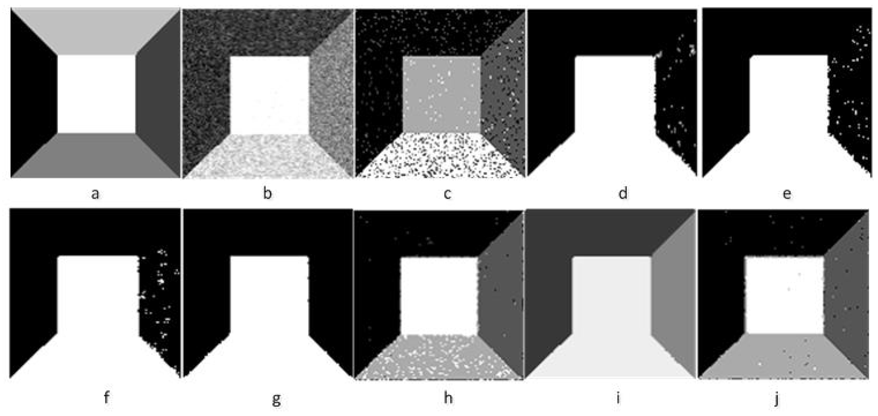
As shown in the Figure 3 below, the synthetic image contains five regions, namely five classes. The gray values of these five regions are respectively 0, 60, 120, 180 and 255. The Figure 3 shows that the different clustering results of several methods under the condition of images with Gaussian noise with the variance: σ g = 20 . It can be observed that KBFWCM produces a better segmentation than the other six fuzzy clustering algorithms. Visually, they can achieve acceptable segmentation results under Gaussian noise. The Figure 3 shows the segmentation accuracies (SAs) of different methods for synthetic images under different noises. Of which, σ g is the variance of Gaussian noise. As can be seen from the first line of Table 3, for synthetic images with different noise levels, the segmentation accuracy of our method is always higher than that of other methods.
As shown in Figure 4, “salt & pepper” noise is added to the synthetic images above to carry out the denoising experiment. This figure shows the clustering denoising results of images with 20 % “salt & pepper” noise. It can be observed that under this condition, KBFWCM produces a better segmentation than the other six fuzzy clustering algorithms. Visually, they can achieve acceptable segmentation results under the “salt & pepper” noise. Table 3 shows the segmentation accuracies (SAs) of different methods for synthetic images under different “salt & pepper" noises. From the Table 3, it can be seen that, for synthetic images with different levels of “salt & pepper” noise, the segmentation accuracy of our method is always higher than that of other methods.

4.3. Comparison of Experimental Results Using Brain MR and Lena Images

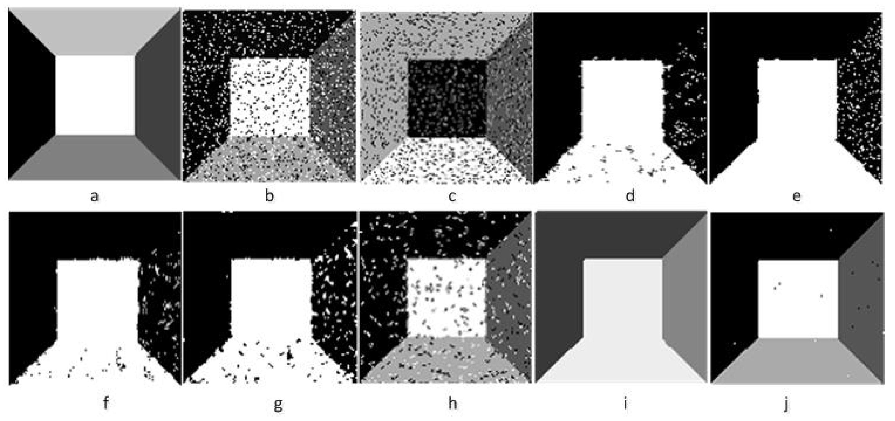
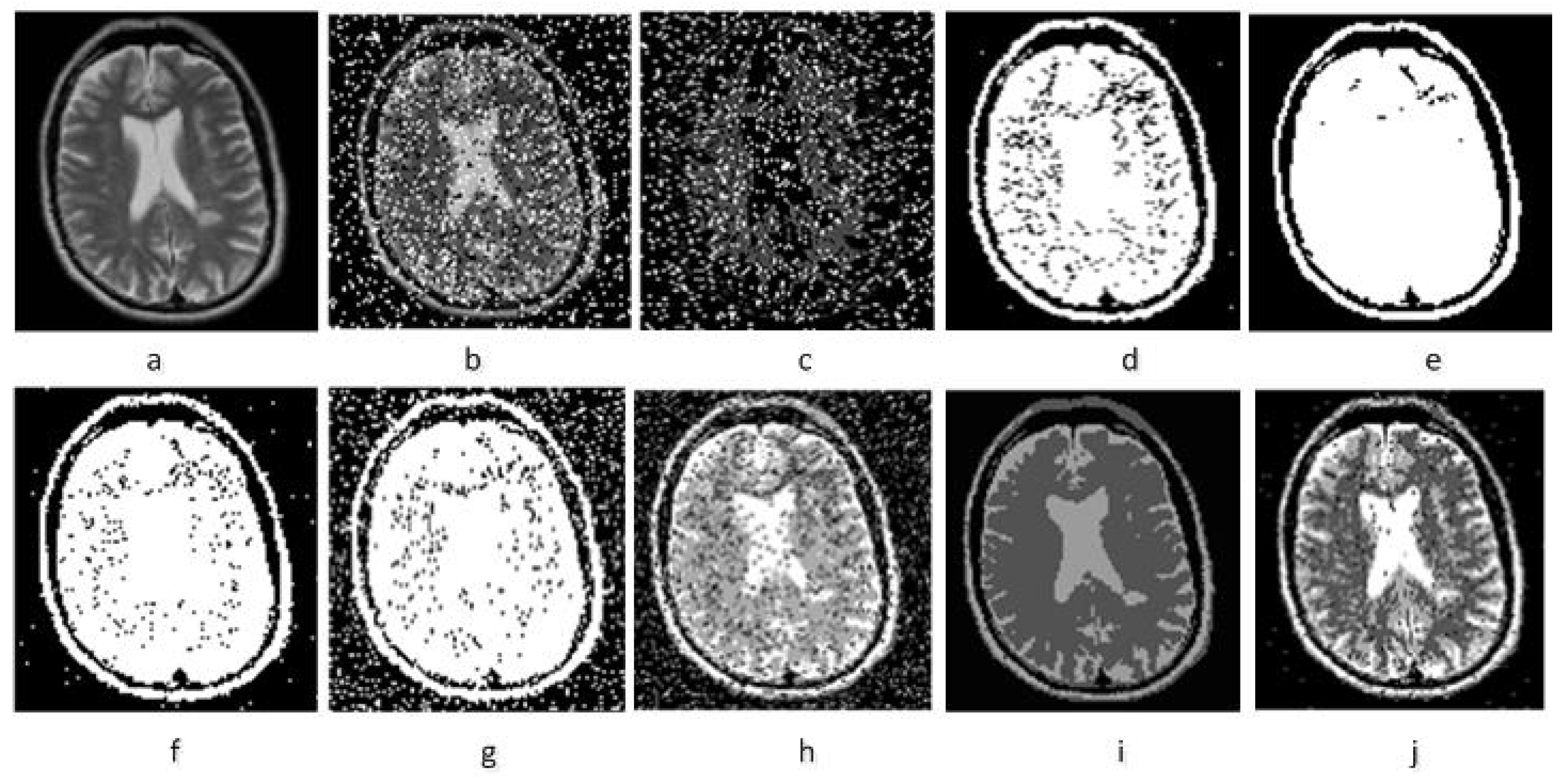
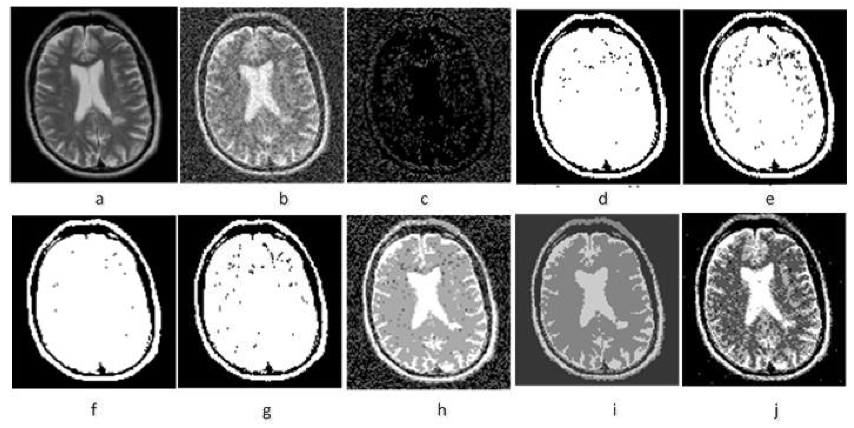
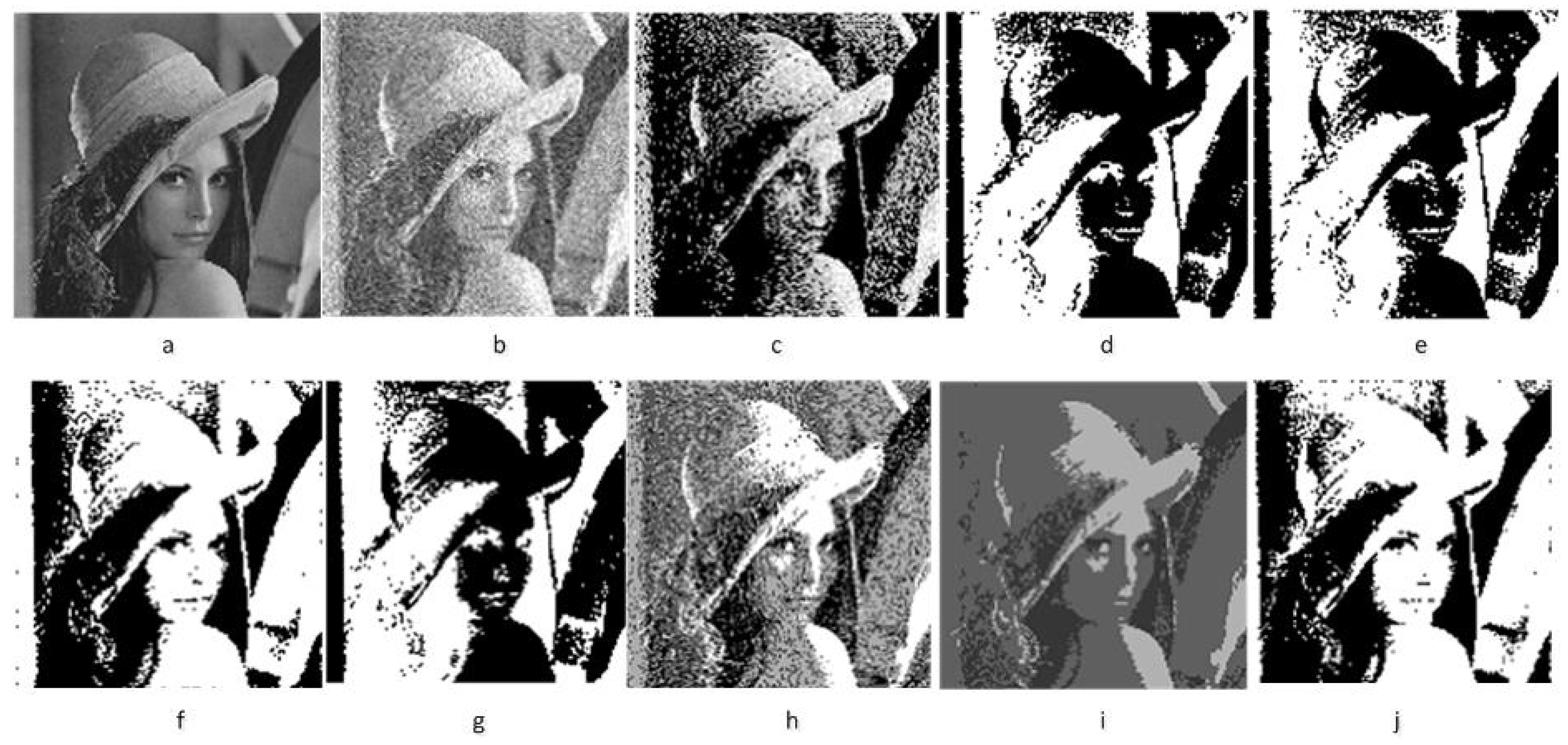
In this section, we experimented with real images, particularly Magnetic Resonance (MR) images and Lena images, in order to prove the performance of the proposed KBFWCM. Meanwhile, some well-known image segmentation methods, such as KFCM, KFCMS1, KFCMS2, KGFCMS, FLICM, ARKFCM and FRFCM, were used as comparison methods. In Figure 3 and Figure 4, the denosing results of synthetic images has been compared. In addition to this, in Figure 5 and Figure 6, we first use Gauss and “salt & pepper” mixture noise to erode the real images [89], then use these 7 algorithms to de-noise real images damaged by noise. Eventually, the comparison is made on the denoising results of real images. The selection of such real images is mainly carried out from two aspects. One is to select MR image for testing, the other is to select the head image of Lena for testing. Such selection also reflects the comparison between medical image and natural portrait.

4.3.1. Denoising Experimental Results of MR Image

The Figure 5c–i shows the denoising segmentation results of different algorithms for images with 20% “salt & pepper” noise. The Figure 6c–i shows the Gaussian denoising segmentation results of various algorithms with σ g = 20 . The segmentation results show that the proposed KBFWCM algorithm can achieve excellent segmentation, while the other fuzzy methods are more or less affected by noise. The FRFCM algorithm is a relatively excellent method, however, it merely considers the influence of traditional fuzzy c-means clustering algorithm and spatial neighborhood but fails to consider the typicality of data attributes. Thus, it is less delicate than KBFWCM algorithm in image denoising.
The parameters in the KBFWCM include the fuzzy control parameter m, size of the neighbourhood N and similarity window S. Roughly speaking, the larger the size of N, the smoother the final results, the larger the similarity window and the more structural information. However, it might use considerably large neighborhood windows and similarity windows for oversmoothing. In the experiment, we find that the 3 × 3 windows of N and S are applicable to brain MR image. For the real Lena images (Figure 7), a larger window is needed to measure the similarity. Under this circumstance, 5 × 5 or 7 × 7 windows of S are applicable. In this paper, a 5 × 5 windows are adopted.

4.3.2. Denoising Experimental Results of Lena’s Head Images

The Figure 7 is a comparison of denoising results on the Lena image with added Gaussian noise with 20 variance. As can be seen from the Figure 7, the proposed KBFWCM algorithm obviously has more advantage than KFCM, KFCMS1, KFCMS2,KGFCMS, FLICM, ARKFCM and FRFCM. The FRFCM algorithm achieves a very good performance in the processing effect but is not better than KBFWCM algorithm in details.
In order to further verify the denoising effect of the KBFWCM algorithm proposed in this paper, the performance of the proposed algorithm is compared and analyzed based on the objective data. Mean Squared Error (MSE), Peak Signal-to-Noise Ratio (PSNR) [90,91] and Signal-to-Noise Ratio (SNR) [92] are used for numerical calculation of the image after denoising.
M S E = 1 M × N i = 1 M j = 1 N f j , i f ^ j i 2
The functions for PSNR and SNR are shown as below:
P S N R = 10 × l o g 10 ( 255 2 M S E ) = 20 · l o g 10 255 M S E
S N R = 10 × l g i = 1 M j = 1 N f j , i 2 / M × N · M S E
Of which, M × N is the size of test image, f j , i and f ^ j i represent the noise-free image and denoised image respectively. The MSE function (29), the PSNR function (30) and SNR function (31) are used for comparison of the image denoised by algorithms in the Figure 7. The calculation results are shown in Table 4 below.
In Table 4,the MSE here is referred as to the mean of the squared sum of gray level difference values of pixel points corresponding to the original image and denoised image. In order to better observe the Mean Squared Error (MSE), the fourth column is provided, in which a percentage is calculated by taking the MSE value of noisy images as the denominator. As can be seen from the fourth column of the Table 4, the smaller the percentage is, the better the denoising effect is, therefore, the performance of KBFWCM is obviously better than that of other algorithms. The smaller the value is, the better the denoised image quality is.
In Table 4, the unit of PSNR is dB. The higher the value of PSNR is, the better the denoising effect is. According to the formula (30) and the formula (31) and by limiting f j , i f ^ j i 2 1 , P S N R 0 , 48.12 after calculation. When the PSNR value here is above 40, it has been close to the original image. Therefore, 31.5349, the PSNR value of the image denoised by the KBFWCOM algorithm, is quite good. SNR means Signal-to-Noise Ratio. The larger its value, the better. By the comparison in the Table 3 above, it can be seen that the denoising effect of KBFWCM algorithm in Lena image is better than that of other algorithms.

5. Conclusions

This paper proposes a fast and robust KBFWCM algorithm for image segmentation to improve image segmentation quality and reduce the impact of image noise. The following things are done:
(1)
The local spatial information of the image and the typicality of the data item are used to improve the segmentation results and the kernel method is used to reduce the computation.
(2)
KBFWCM uses the membership filtering algorithm to exploit the local spatial constraint. Since noise points will have low compatibility in all clusters, the membership functions obtained by this algorithm more approach to the concept of typicality, making their impact on clustering negligible. Therefore, this algorithm is naturally more immune to noise.
(3)
This algorithm has additional advantages in calculation. It is a natural mechanism, assigning ’fuzzy labels’ to data in each iteration. Therefore, it can be used for more complex pattern recognition.
(4)
Experimental results show that the proposed KBFWCM can provide better segmentation results without adjusting parameters for different grayscale.

Author Contributions

All authors discussed the required algorithm to complete the manuscript. W.Z. and X.G. conceived the paper. W.Z. and T.H. performed the experiments and wrote the paper. J.L. and J.C. checked for typographical errors.

Funding

This work is funded Natural Science Foundation of Hebei Province, China (Grant no. E2017203351). The work is also funded by Scientific Research Foundation of YanShan University.

Acknowledgments

An Acknowledgements section is optional and may recognise those individuals who provided help during the research and preparation of the manuscript.

Conflicts of Interest

The authors declare that there are no conflict of interest regarding the publication of this paper.

References

  1. Sghaier, G. A K-Means Clustering-Based Security Framework for Mobile Data Mining. Wirel. Commun. Mob. Comput. 2016, 16, 3449–3454. [Google Scholar]
  2. Subbalakshmi, C.; Ramakrishna, G.; Rao, S.K.M. Evaluation of Data Mining Strategies Using Fuzzy Clustering in Dynamic Environment. In Proceedings of the 3rd International Conference on Advanced Computing, Networking and Informatics, Orissa, India, 23–25 June 2016; pp. 529–536. [Google Scholar]
  3. Wan, L.; Zhang, T.; Xiang, Y.M. A Robust Fuzzy C-means Algorithm Based on Bayesian Nonlocal Spatial information for SAR Image Segmentation. IEEE J. Sel. Top. Appl. Earth Obs. Remote Sens. 2018, 11, 896–906. [Google Scholar] [CrossRef]
  4. Gharieb, R.; Gendy, G.; Selim, H. A Hard CMeans Clustering Algorithm Incorporating Membership KL Divergence And Local Data Information for Noisy Image Segmentation. Int. J. Pattern Recognit. Artif. Intell. 2018, 32, 758–769. [Google Scholar] [CrossRef]
  5. Naz, S.; Majeed, H.; Irshad, H. Image segmentation using fuzzy clustering: A survey. In Proceedings of the IEEE International Conference on Emerging Technologies, Cagliari, Italy, 10–13 September 2013; Volume 2, pp. 2927–2929. [Google Scholar]
  6. Ouma, Y.O.; Hahn, M. Pothole Detection on Asphalt Pavements from 2D-Colour Pothole Images Using Fuzzy C-means Clustering and Morphological Reconstruction. Autom. Constr. 2017, 83, 196–211. [Google Scholar] [CrossRef]
  7. Baraldi, A.; Blonda, P. A survey of fuzzy clustering algorithms for pattern recognition I. IEEE Syst. Man Cybern. Soc. 1999, 29, 778–785. [Google Scholar] [CrossRef] [PubMed]
  8. Shabia, S.K.; Quadri, S.M.K. Structure Identification and IO Space Partitioning In a Nonlinear Fuzzy System for Prediction of Patient Survival after Surgery. Int. J. Intell. Comput. Cybern. 2017, 10, 166–182. [Google Scholar]
  9. Huang, H.C.; Chuang, Y.Y.; Chen, C.S. Multiple Kernel Fuzzy Clustering. IEEE Trans. Fuzzy Syst. 2012, 20, 120–134. [Google Scholar] [CrossRef]
  10. Masulli, F.; Rovetta, S. Soft Transition from Probabilistic to Possibilistic Fuzzy Clustering. IEEE Trans. Fuzzy Syst. 2006, 14, 516–527. [Google Scholar] [CrossRef]
  11. Cao, H.; Deng, H.W.; Wang, Y.P. Segmentation of M-FISH Images for Improved Classification of Chromosomes with an Adaptive Fuzzy C-means Clustering Algorithm. IEEE Trans. Fuzzy Syst. 2012, 20, 1–8. [Google Scholar] [CrossRef]
  12. Javed, A.; Kim, Y.C.; Khoo, M.C.K.; Ward, S.L.D.; Nayak, K.S. Dynamic 3D MR Visualization and Detection of upper Airway Obstruction during Sleep Using Region Growing Segmentation. IEEE Trans. Biomed. Eng. 2016, 63, 431–437. [Google Scholar] [CrossRef]
  13. Grau, V.; Mewes, A.U.J.; Alcaniz, M.; Kikinis, R.; Warfield, S.K. Improved Watershed Transform for Medical Image Segmentation Using Prior Information. IEEE Trans. Med. Imaging 2004, 23, 447–458. [Google Scholar] [CrossRef] [PubMed]
  14. Gong, M.; Li, H.; Zhang, X.; Zhao, Q.; Wang, B. Nonparametric Statistical Active Contour Based on Inclusion Degree of Fuzzy Sets. IEEE Trans. Fuzzy Syst. 2016, 24, 1176–1192. [Google Scholar] [CrossRef]
  15. Comaniciu, D.; Meer, P. Mean Shift: A Robust Approach toward Feature Space Analysis. IEEE Trans. Pattern Anal. Mach. Intell. 2002, 24, 603–619. [Google Scholar] [CrossRef]
  16. Mahapatra, D. Semi-Supervised Learning and Graph Cuts for Consensus Based Medical Image Segmentation. Pattern Recognit. 2017, 5, 700–709. [Google Scholar] [CrossRef]
  17. Li, Z.; Chen, J. Super pixel Segmentation Using Linear Spectral Clustering. In Proceedings of the IEEE Conference Computer Vision Pattern Recognition (CVPR), Boston, MA, USA, 7–12 June 2015; Volume 10, pp. 1356–1363. [Google Scholar]
  18. Chatzis, S.P.; Varvarigou, T.A. A Fuzzy Clustering Approach Toward Hidden Markov Random Field Models for Enhanced Spatially Constrained Image Segmentation. IEEE Trans. Fuzzy Syst. 2008, 16, 1351–1361. [Google Scholar] [CrossRef]
  19. Pathak, D.; Krahenbuhl, P.; Darrell, T. Constrained Convolutional Neural Networks for Weakly Supervised Segmentation. In Proceedings of the IEEE International Conference on Computer Vision (ICCV), Santiago, Chile, USA, 7–13 December 2015; pp. 2380–7504. [Google Scholar]
  20. Wang, B.; Tu, Z. Affinity Learning via Self-Diffusion for Image Segmentation and Clustering. In Proceedings of the IEEE Conference Computer Vision Pattern Recognition (CVPR), Providence, RI, USA, 16–21 June 2012; pp. 2312–2319. [Google Scholar]
  21. Kim, S.; Yoo, C.D.; Nowozin, S.; Kohli, P. Image Segmentation Using Higher-Order Correlation Clustering. IEEE Trans. Pattern Anal. Mach. Intel. 2014, 36, 1761–1774. [Google Scholar] [CrossRef] [PubMed]
  22. Pont-Tuset, J.; Arbelaez, P.; Barron, J.; Marques, F.; Malik, J. Multiscale Combinatorial Grouping for Image Segmentation and Object Proposal Generation. IEEE Trans. Pattern Anal. Mach. Intell. 2017, 39, 128–140. [Google Scholar] [CrossRef] [PubMed]
  23. Hasnat, M.A.; Alata, O. Joint Color- Spatial-Directional Clustering and Region Merging (JCSDRM) for Unsupervised RGB-D Image Segmentation. IEEE Trans. Pattern Anal. Mach. Intell. 2016, 38, 2255–2268. [Google Scholar] [CrossRef]
  24. Bampis, C.G.; Maragos, P.; Bovik, A.C. Graph-Driven Diffusion and Random Walk Schemes for Image Segmentation. IEEE Trans. Image Process. 2017, 26, 35–50. [Google Scholar] [CrossRef]
  25. Saha, P.K.; Basu, S.; Hoffman, E.A. Multiscale Opening of Conjoined Fuzzy Objects: Theory and Applications. IEEE Trans. Fuzzy Syst. 2016, 24, 1121–1133. [Google Scholar] [CrossRef]
  26. Dunnt, J.C. Well-Separated Clusters and Optimal Fuzzy Partitions. J. Cybern. 2008, 4, 95–104. [Google Scholar]
  27. Dunn, J.C. A fuzzy relative of the ISODATA Process and Its Use in Detecting Compact Well-Separated Clusters. J. Cybern. 1973, 3, 32–57. [Google Scholar] [CrossRef]
  28. Dunnt, J.C. Some Recent Investigations of a New Fuzzy Partitioning Algorithm and Its Application to Pattern Classification Problems. J. Cybern. 1974, 4, 1–15. [Google Scholar]
  29. Zadeh, L.A. Fuzzy sets. Inf. Control 1965, 8, 338–353. [Google Scholar] [CrossRef] [Green Version]
  30. Gitman, I.; Levine, M.D. An Algorithm for Detecting Unimodal Fuzzy Sets and Its Application as a Clustering Technique. IEEE Comput. Soc. 1970, 100, 583–593. [Google Scholar] [CrossRef]
  31. Bezdek, J.C. Cluster Validity with Fuzzy Sets. J. Cybern. 1974, 3, 58–73. [Google Scholar] [CrossRef]
  32. Bezdek, J.C. Numerical Taxonomy with Fuzzy Sets. J. Math. Biol. 1974, 10, 57–71. [Google Scholar] [CrossRef]
  33. Bezdek, J.C. Convex Decompositions of Fuzzy Partitions. J. Math. Anal. Appl. 1979, 10, 490–512. [Google Scholar] [CrossRef]
  34. Bezdek, J.C. A Convergence Theorem for the Fuzzy C-means Clustering Algorithms. IEEE Trans. PAMI 1980, 2, 1–8. [Google Scholar] [CrossRef]
  35. Bezdek, J.C. Pattern Recognition with Fuzzy Objective Function Algorithms. Adv. Appl. Pattern Recognit. 1981, 22, 203–239. [Google Scholar]
  36. Bezdek, J.C.; Trivedi, M.; Ehrlich, R.; Full, W. Fuzzy Clustering: A New Approach for Geostatistical Analysis. Syst. Meas. Decis. 1982, 10, 142–149. [Google Scholar]
  37. Bezdek, J.C.; Ehrlich, R.; Full, W. FCM: The Fuzzy C-means Clustering Algorithm. Comput. Geosci. 1984, 10, 191–203. [Google Scholar] [CrossRef]
  38. Pal, N.; Bezdek, J. On cluster validity for the fuzzy c-means model. IEEE Trans. Fuzzy Syst. 1995, 3, 370–379. [Google Scholar] [CrossRef]
  39. Gong, M.; Su, L.; Jia, M.; Chen, W. Fuzzy Clustering With a Modified MRF Energy Function for Change Detection in Synthetic Aperture Radar Images. IEEE Trans. Fuzzy Syst. 2014, 22, 98–109. [Google Scholar] [CrossRef]
  40. Chiang, I.J.; Liu, C.H.; Tsai, Y.H.; Kumar, A. Discovering Latent Semantics in Web Documents using Fuzzy Clustering. IEEE Trans. Fuzzy Syst. 2015, 23, 2122–2134. [Google Scholar] [CrossRef]
  41. Nguyen, T.; Wu, J. Online feature selection based on fuzzy clustering and its applications. IEEE Trans. Fuzzy Syst. 2016, 24, 1294–1306. [Google Scholar] [CrossRef]
  42. Hu, L.; Chan, K.C. Fuzzy clustering in a complex network based on content relevance and link structures. IEEE Trans. Fuzzy Syst. 2016, 24, 456–470. [Google Scholar] [CrossRef]
  43. Krishnapuram, R.; Keller, J.M. A possibilistic approach to clustering. IEEE Trans. Fuzzy Syst. 1993, 1, 98–110. [Google Scholar] [CrossRef]
  44. Krishnapuram, R.; Keller, J.M. The possibilistic C-means algorithm: Insights and recommendations. IEEE Trans. Fuzzy Syst. 1996, 4, 385–393. [Google Scholar] [CrossRef]
  45. Pal, N.R.; Pal, K.; Bezdek, J.C. A mixed C-means clustering model. In Proceedings of the IEEE International Conference on Fuzzy Systems, Barcelona, Spain, 5– July 1997; Volume 1, pp. 11–21. [Google Scholar]
  46. Pal, N.R.; Pal, K.; Keller, J.M.; Bezdek, J.C. A Possibilistic Fuzzy C-means Clustering Algorithm. IEEE Trans. Fuzzy Syst. 2005, 13, 517–530. [Google Scholar] [CrossRef]
  47. Dunn, J.C. A Fuzzy Relative of the ISODATA Process and Its Use in Detecting Compact Well-Separated Clusters Department of Theoretical and Applied Mechanics. J. Cybern. 1974, 3, 32–57. [Google Scholar] [CrossRef]
  48. Tolias, Y.A.; Panas, S.M. Image Segmentation by a Fuzzy Clustering Algorithm Using Adaptive Spatially Constrained Membership Functions. IEEE Trans. SMC-PART A 1998, 28, 359–369. [Google Scholar] [CrossRef]
  49. Ahmed, M.N.; Yamany, S.M.; Mohamed, N.; Farag, A.A.; Moriarty, T. A Modified Fuzzy C-means Algorithm for Bias Field Estimation and Segmentation of MRI Data. IEEE Trans. Med. Imaging 2002, 21, 193–199. [Google Scholar] [CrossRef] [PubMed]
  50. Pham, D.L. Spatial Models for Fuzzy Clustering. Comput. Vis. Image Underst. 2001, 84, 295–297. [Google Scholar] [CrossRef]
  51. Liew, A.W.C.; Leung, S.H.; Lau, W.H. Fuzzy Image Clustering Incorporating Spatial Continuity. IEEE Proc. Vis. Image Signal Process. 2000, 147, 185–192. [Google Scholar] [CrossRef]
  52. Chuang, K.; Tzeng, H.; Chen, S.; Wu, J.; Chen, T.J. Fuzzy c-means clustering with spatial information for image segmentation. Comput. Med. Imaging Graph. 2006, 30, 9–15. [Google Scholar] [CrossRef] [Green Version]
  53. Chen, S.; Zhang, D. Robust image segmentation using FCM with spatial constraints based on new kernel-induced distance measure. IEEE Trans. Syst. Man Cybern. Part B 2004, 34, 1907–1916. [Google Scholar] [CrossRef]
  54. Szilagyi, L.; Benyo, Z.; Szilagyi, S.M.; Adam, H.S. MR Brain Image Segmentation Using an Enhanced Fuzzy CMeans Algorithm. In Proceedings of the International Conference of the IEEE Engineering in Medicine & Biology Society, Milano, Italy, 25–29 August 2003; Volume 10, pp. 724–726. [Google Scholar]
  55. Cai, W.L.; Chen, S.C.; Zhang, D.Q. Fast And Robust Fuzzy C-means Clustering Algorithms Incorporating Local Information For Image Segmentation. Pattern Recognit. 2007, 40, 825–838. [Google Scholar] [CrossRef]
  56. Hathaway, R.J.; Bezdek, J.C.; Hu, Y.H.Y. Generalized fuzzy c-means clustering strategies using Lp norm distances. IEEE Trans. Fuzzy Syst. 2000, 8, 576–582. [Google Scholar] [CrossRef]
  57. Zhu, L.; Chung, F.L.; Wang, S. Generalized Fuzzy C-Means Clustering Algorithm With Improved Fuzzy Partitions. J. Comput. Res. Dev. 2009, 39, 578–591. [Google Scholar]
  58. Crammer, K.; Singer, Y. On the Algorithmic Implementation of Multiclass Kernel-based Vector Machines. J. Mach. Learn. Res. 2002, 2, 265–292. [Google Scholar]
  59. Yang, X.; Zhang, G.; Lu, J.; Ma, J. A Kernel Fuzzy c-Means Clustering-Based Fuzzy Support Vector Machine Algorithm for Classification Problems With Outliers or Noises. IEEE Trans. Fuzzy Syst. 2014, 10, 105–115. [Google Scholar] [CrossRef]
  60. Zhao, F.; Jiao, L.; Liu, H. Kernel generalized fuzzy C-means clustering with spatial information for image segmentation. Digit. Signal Process 2013, 23, 184–199. [Google Scholar] [CrossRef]
  61. Yang, M.S.; Tsai, H.S. A Gaussian Kernel-Based Fuzzy C-means Algorithm with a Spatial Bias Correction. Pattern Recognit. Lett. 2008, 29, 1713–1725. [Google Scholar] [CrossRef]
  62. Wang, J.Z.; Kong, J.; Lu, Y.H.; Qi, M.; Zhang, B.A. Modified FCM Algorithm for MRI Brain Image Segmentation Using Both Local and Non-Local Spatial Constraints. Comput. Med. Imaging Graph. 2008, 32, 685–698. [Google Scholar] [CrossRef] [PubMed]
  63. Krinidis, S.; Chatzis, V. A Robust Fuzzy Local Information C-means Clustering Algorithm. IEEE Trans. Image Process. 2010, 19, 1328–1337. [Google Scholar] [CrossRef]
  64. Gong, M.; Zhou, Z.; Ma, J. Change Detection in Synthetic Aperture Radar Images Based on Image Fusion and Fuzzy Clustering. IEEE Trans. Image Process. 2012, 21, 2141–2151. [Google Scholar] [CrossRef]
  65. Elazab, A.; Wang, C.; Jia, F.; Wu, J.; Li, G.; Hu, Q. Segmentation of Brain Tissues from Magnetic Resonance Images Using Adaptively Regularized Kernel-Based Fuzzy C-Means Clustering. Comput. Math. Methods Med. 2015, 5, 1–12. [Google Scholar] [CrossRef]
  66. Lei, T.; Jia, X.; Zhang, Y.; He, L.; Meng, H.; Nandi, A.K. Significantly Fast and Robust Fuzzy C-means Clustering Algorithm Based on Morphological Reconstruction and Membership Filtering. IEEE Trans. Fuzzy Syst. 2018, 26, 3027–3041. [Google Scholar] [CrossRef]
  67. Saranathan, A.M.; Parente, M. Uniformity-Based Superpixel Segmentation of Hyperspectral Images. IEEE Trans. Geosci. Remote Sens. 2016, 54, 1419–1430. [Google Scholar] [CrossRef]
  68. Zhao, Z.; Lizhi, C.; Guangquan, C. Neighbourhood Weighted Fuzzy C-means Clustering Algorithm for Image Segmentation. IET Image Process. 2014, 8, 150–161. [Google Scholar]
  69. Guo, F.; Wang, X.; Shen, J. Adaptive Fuzzy C-means Algorithm Based on Local Noise Detecting for Image Segmentation. IET Image Process. 2016, 10, 272–279. [Google Scholar] [CrossRef]
  70. Jacek, M.L. Fuzzy C-Ordered Means Clustering. Fuzzy Sets Syst. 2016, 10, 114–133. [Google Scholar]
  71. Huber, P.J. Robust Covariance and Correlation Matrices. In Robust Statistics; Wiley: New York, NY, USA, 1981; pp. 199–204. [Google Scholar]
  72. Yager, R.R. On Ordered Weighted Averaging Aggregation Operators in Multicriteria Decision Making. IEEE Trans. Syst. Man Cybern. 1988, 18, 183–190. [Google Scholar] [CrossRef]
  73. Krzysztof, S. Fuzzy Weighted C-Ordered Means Clustering Algorithm. Fuzzy Sets Syst. 2017, 318, 1–33. [Google Scholar]
  74. Muller, K.R.; Mika, S. An introduction to kernel-based learning algorithms. IEEE Trans. Neural Netw. 2001, 12, 181–202. [Google Scholar] [CrossRef] [PubMed]
  75. Cristianini, N.L. 3-Kernel-Induced Feature Spaces. In Support Vector Machines; Taylor, J.S., Ed.; Cambridge University: London, UK, 2013; pp. 26–51. [Google Scholar]
  76. Vapnik, V.N. Support Vector Learning Machines. In Statistical Learning Theory; Simon, H., Ed.; Wiley: New York, NY, USA, 1998; pp. 375–380. [Google Scholar]
  77. Scholkopf, B.L. Incorporating invariances in support vector learning machines. In Artificial Neural Networks-ICANN 96; Scholkopf, B., Burges, C., Vapnik, V., Eds.; Springer: Berlin/Heidelberg, Germany, 1996; pp. 47–52. [Google Scholar]
  78. Volker, R.; Volker, S.L. Nonlinear Discriminant Analysis Using Kernel Functions. In Advances Neural Information Processing Systems 12; Solla, S.A.F., Leen, T.K., Muller, K.R., Eds.; MIT Press: Cambridge, MA, USA, 2000; pp. 568–574. [Google Scholar]
  79. Scholkopf, B.; Smola, A.; Muller, K.-R. Nonlinear Component Analysis as a Kernel Eigenvalue Problem. Neural Comput. 1998, 10, 1299–1319. [Google Scholar] [CrossRef] [Green Version]
  80. Chen, J.H.; Chen, C.S. Fuzzy kernel perceptron. EEE Trans. Neural Netw. 2002, 13, 1364–1373. [Google Scholar] [CrossRef] [PubMed]
  81. Girolami, M. Mercer kernel-based clustering in feature space. IEEE Trans. Neural Netw. 2002, 10, 780–784. [Google Scholar] [CrossRef]
  82. Zhang, D.Q.; Chen, S.C. Fuzzy clustering using kernel methods. In Proceedings of the International Conference Control Automation, Xiamen, China, 19 June 2002; Volume 10, pp. 123–127. [Google Scholar]
  83. Zhang, D.Q.; Chen, S.C. Clustering Incomplete Data Using Kernel-Based Fuzzy C-means Algorithm. Neural Process. Lett. 2003, 18, 155–162. [Google Scholar] [CrossRef]
  84. Cristianini, N.; Shawetaylor, J. An Introduction to Support Vector Machines and Other Kernel-based Learning Methods. Kybernetes 2001, 32, 1–28. [Google Scholar]
  85. Bernhard, S. Kernel Principal Component Analysis. In Advances in Kernel Methods-Support Vector Learning; Christopher, J.C., Alexauder, J.S., Eds.; Springer: Berlin/Heidelberg, Germany, 2007; pp. 327–373. [Google Scholar]
  86. Rasmussen, C.E.; Williams, C.K.I. Gaussian processes in machine learning. In Summer School on Machine Learning; Springer: Berlin/Heidelberg, Germany, 2006; Volume 10, pp. 67–75. [Google Scholar]
  87. Wu, Z.D.; Xie, W.X.; Yu, J.P. Fuzzy C-means Clustering Algorithm based on Kernel Method. In Proceedings of the 15th International Conference on Computational Intelligence and Multimedia Applications, Las Vegas, NV, USA, 16–18 August 2003; Volume 10, pp. 49–54. [Google Scholar]
  88. Wu, K.L.; Yang, M.S. Alternative C-means clustering algorithms. Pattern Recognit. 2002, 35, 2267–2278. [Google Scholar] [CrossRef]
  89. Mathworks, N.M. Image Processing Toolbox. Available online: http://www.mathworks.Com (accessed on 4 June 2017).
  90. Sanjith, S. Fusion of DWT-DCT algorithm for satellite image compression. Int. J. Appl. Eng. Res. 2015, 10, 130–137. [Google Scholar]
  91. Sanjith, S.; Ganesan, R.; Rimal, I.R.S. Experimental Analysis of Compacted Satellite Image Quality Using Different Compression Methods. Adv. Sci. Eng. Med. 2015, 7, 227–233. [Google Scholar] [CrossRef]
  92. Cavouras, D.; Kandarakis, I.; Kanellopoulos, M.; Nomicos, C.D.; Panayiotakis, G.S. Signal-to-noise-ratio (SNR) of X-ray imaging scintillators determined by luminescence measurements. Appl. Radiat. Isot. 1999, 51, 59–68. [Google Scholar] [CrossRef]
Figure 1. The though origin of the Kernel-based Robust Bias-correction Fuzzy Weighted C-ordered-means Clustering Algorithm (KBFWCM) algorithm.
Symmetry 11 00753 g001
Figure 2. The piecewise linear ordered weighted averaging (PLOWA) and S-ordered weighted average (SOWA) weighting functions for n = 100 and p a = 0.2 , p c = 0.5 , p l = 0.2 .
Symmetry 11 00753 g002
Figure 3. Comparison of segmentation results on the synthetic image from denoising base on Gaussian. (a) Ground truth image; (b) The image added Gaussian (zero mean and 20 variance); (c) KFCM result; (d) KFCMS1 result; (e) KFCMS2 result; (f) KGFCMS; (g) FLICM result; (h) ARKFCM result; (i) FRFCM result;(j) KBFWCM result.
Symmetry 11 00753 g003
Figure 4. Comparison of segmentation results on the synthetic image from denoising base on salt & pepper. (a) Ground truth image; (b) The image added salt & pepper (zero mean and 20 % variance); (c) KFCM result; (d) KFCMS1 result; (e) KFCMS2 result; (f) KGFCMS; (g) FLICM result; (h) ARKFCM result; (i) FRFCM result;(j) KBFWCM result.
Symmetry 11 00753 g004
Figure 5. Comparison of segmentation results on the brain MR image from denoising base on salt & pepper. (a) Ground truth image; (b) The image added salt & pepper (zero mean and 20 % variance); (c) KFCM result; (d) KFCMS1 result; (e) KFCMS2 result; (f) KGFCMS; (g) FLICM result; (h) ARKFCM result; (g) FLICM result; (h) ARKFCM result; (i) FRFCM result;(j) KBFWCM result.
Symmetry 11 00753 g005
Figure 6. Comparison of segmentation results on the brain MR image from denoising base on Gaussian. (a) Ground truth image; (b) The image added Gaussian (zero mean and 20 variance); (c) KFCM result; (d) KFCMS1 result; (e) KFCMS2 result; (f) KGFCMS; (g) FLICM result; (h) ARKFCM result; (i) FRFCM result; (j) KBFWCM result.
Symmetry 11 00753 g006
Figure 7. Comparison of segmentation results on the Lena image from denoising base on Gaussian. (a) Ground truth image; (b) The image added Gaussian (zero mean and 20 variance); (c) KFCM result; (d) KFCMS1 result; (e) KFCMS2 result; (f) KGFCMS; (g) FLICM result; (h) ARKFCM result; (i) FRFCM result; (j) KBFWCM result.
Symmetry 11 00753 g007
Table 1. Theoretical Formulations of Classical fuxxy c-means (FCM) Algorithm and some of its improved versions.
Algorithm NameAbbreviationObjective FunctionTime
Fuzzy C-Means [37]FCM J m = i = 1 c k = 1 n u i k m x k v i 2 1984
FCM with spatial constraints [49]FCMS J m = i = 1 c j = 1 n u i j m x j v i 2 + α N R i = 1 c j = 1 n u i j m r N i x r v i 2 2002
Enhanced FCM [54]EnFCM J m = i = 1 c j = 1 l u i j m ξ j v i 2 , ξ j = α 1 + α x j + α N R r N j x r . 2003
Two variants of FCMS [53]FCMS1 FCMS2 J m = i = 1 c j = 1 n u i j m x j v i 2 + α N R i = 1 c j = 1 n u i j m x ¯ j v i 2 2004
Spatial FCM [52]SFCM J = j = 1 N i = 1 c u i j m x j v i 2 W h e r e h i j = k N B ( x j ) u i k , u i j = u i j p h i j q k = 1 c u k j p h k j q . 2006
Fuzzy Local Information C-Means [64]FLICM J m = i = 1 c j = 1 n u i j m x j v i 2 + G i j W h e r e , G i j = α N R r N j , j r 1 1 + d j r 1 u i j m x r v i 2 2012
Two Kernel variants of GIFPFCM [60]KGFCMS1 KGFCMS2 J m = 2 i = 1 c j = 1 n u i j m 1 K x j , v i + j = 1 n a j i = 1 c u i j 1 u i j m 1 + 2 β i = 1 c j = 1 n u i j m 1 K x ¯ j , v i 2013
New Weighted Fuzzy C-Means [68]NWFCM J m = i = 1 c k = 1 n u i k m x j M i j 2 W h e r e , M i j = r = 1 , r j n x j x r 1 u i r x r r = 1 , r j n x j x r 1 u i r x r r = 1 , r j n x j x r 1 u i r r = 1 , r j n x j x r 1 u i r 2014
Adaptively Regularized Kernel-based FCM [69]ARKFCM J A R K F C M = 2 i = 1 N j = 1 c u i j m 1 K x i , v j + i = 1 N j = 1 c φ i u i j m 1 K x ¯ i , v j 2016
Fuzzy C-Ordered-Means [70]FCOM J ( U , V ) = i = 1 c k = 1 N β i k ( u i k ) m D ( x k , v i ) , W h e r e , D ( x k , v i ) = x k v i A 2 = ( x k v i ) T A ( x k v i ) . 2016
Fuzzy weighted C-ordered-means [73]FWCOM J U , V , Z = c = 1 C i = 1 X β c i u c i m d = 1 D z c d ϕ x i d v c d 2 , W h e r e , c C , d = 1 D z c d = 1 , k X , c = 1 C β c k u c k = f k . 2017
Reconstruction and membership Filtering FCM [66]FRFCM J m = l = 1 q k = 1 c γ l u k l m ζ l v k 2 , l = 1 q γ l = N 2018
Table 2. Classification effect of FCM algorithm, FCMS algorithm and BFWCOM algorithm on IRIS data.
AlgorithmMisclassification NumbersCERClustering CenterDD
FCM1610.7% v 1 = ( 5.0040 , 3.4141 , 1.4828 , 0.2535 ) v 2 = ( 5.8887 , 2.7610 , 4.3636 , 1.3972 ) v 3 = ( 6.7748 , 3.0523 , 5.6465 , 2.0534 ) 0.081
FCMS106.7% v 1 = ( 4.9940 , 3.3649 , 1.4833 , 0.2537 ) v 2 = 5.7787 , 2.7851 , 4.2636 , 1.3882 v 3 = ( 6.6648 , 3.0573 , 5.6485 , 2.0564 ) 0.063
KFCMS96% v 1 = ( 4.9834 , 3.3781 , 1.5033 , 0.2641 ) v 2 = 5.6772 , 2.8001 , 4.3023 , 1.3872 v 3 = ( 6.7101 , 3.1001 , 5.7023 , 2.1032 ) 0.057
FWCOM85.3% v 1 = 4.9940 , 3.3649 , 1.4833 , 0.2537 v 2 = 5.7787 , 2.7851 , 4.2636 , 1.3882 v 3 = ( 6.6648 , 3.0573 , 5.6485 , 2.0564 ) 0.049
ARKFCM74.7% v 1 = 4.9840 , 3.3549 , 1.4533 , 0.2497 v 2 = ( 5.7817 , 2.8051 , 4.2539 , 1.3082 ) v 3 = ( 6.3948 , 3.0583 , 5.3485 , 2.0821 ) 0.046
FRFCM53.3% v 1 = 4.9941 , 3.3650 , 1.4863 , 0.2577 v 2 = ( 5.7767 , 2.7853 , 4.2615 , 1.2782 ) v 3 = ( 6.4648 , 3.0893 , 5.3485 , 2.1564 ) 0.037
KBFWCM53.3% v 1 = 4.9969 , 3.3649 , 1.4623 , 0.2158 v 2 = ( 5.7723 , 2.7852 , 4.1582 , 1.2782 ) v 3 = ( 6.4490 , 2.9253 , 5.4026 , 2.0110 ) 0.035
Table 3. Comparison of segmentation accuracies (%) on synthetic images degraded by different noise.
Algorithm σ g = 10 σ g = 20 σ g = 25Salt & Pepper (5%)Salt & Pepper (10%)Salt & Pepper (20%)
KFCM85.9486.1685.3492.7193.4195.35
KFCMS186.0786.1787.0593.6894.5695.78
KFCMS289.1587.4086.4494.6895.8594.89
KGFCMS71.5094.7494.9098.8496.9799.32
FLICM96.6496.6496.6497.3496.4497.28
ARKFCM93.1793.1793.1794.2395.8497.84
FRFCM97.8498.7896.9795.9696.9497.92
KBFWCM98.9198.9397.8698.3597.7797.98
Table 4. Noise-free Lena image denoising effect evaluation index (n = 3, δ = 0.2 ).
Denosing MethodMSEMSE % PSNR/dbSNR/db
Image with noise640.546110020.065313.4480
KFCM138.611921.6426.712821.0557
KFCMS1179.675228.0526.131420.0553
KFCMS2182.473728.4925.518819.8616
KGFCMS105.483616.4726.012520.6052
FLICM107.173916.7326.167020.5099
ARKFCM91.492214.2828.898622.2414
FRRCM67.506610.5429.542523.8853
KBFWCM54.90238.5331.534924.6808