Article

Stereographic Visualization of 5-Dimensional Regular Polytopes

1
School of Mathematics and Physics, Jinggangshan University, Ji’an 343009, China
2
Department of Mathematics, City University of Hong Kong, Kowloon, Hong Kong
3
Institute of Mathematics, University of Silesia, 40-007 Katowice, Poland
*
Author to whom correspondence should be addressed.
Symmetry 2019, 11(3), 391; https://doi.org/10.3390/sym11030391
Submission received: 30 January 2019 / Revised: 12 March 2019 / Accepted: 15 March 2019 / Published: 18 March 2019

Abstract

:
Regular polytopes (RPs) are an extension of 2D (two-dimensional) regular polygons and 3D regular polyhedra in n-dimensional ( n 4 ) space. The high abstraction and perfect symmetry are their most prominent features. The traditional projections only show vertex and edge information. Although such projections can preserve the highest degree of symmetry of the RPs, they can not transmit their metric or topological information. Based on the generalized stereographic projection, this paper establishes visualization methods for 5D RPs, which can preserve symmetries and convey general metric and topological data. It is a general strategy that can be extended to visualize n-dimensional RPs ( n > 5 ).

1. Introduction

Regular polytopes (RPs) are an extension of 2D regular polygons and 3D regular polyhedra in n-dimensional Euclidean space R n ( n 4 ), which have high abstraction and perfect symmetry [1,2,3]. For instance, the 5D hypercube { 4 , 3 , 3 , 3 } has 32 vertices, 80 edges, 80 squares, 40 3D cubes, and 10 4D regular polytopes { 4 , 3 , 3 } . Those vertices, edges, squares, cubes, and 4D cells combine together to form a very coordinated and symmetrical structure, which in total consists of 1920 symmetries. The strong symmetrical structure of RPs thus gives them an aesthetic quality that has had a continuous and deep influence in the fields of math, computer graphics, art, and commercial design [4,5,6,7,8].
The history of scientific and technological progress shows that the study of symmetry is of great significance [9,10]. It has greatly promoted the integration and development of natural sciences and has a far-reaching impact in practical fields. For example, the research of 2D symmetries produces the profound result of planar symmetry groups, which is widely used in the fields of architecture and decoration [4,11,12]. The study of 3D symmetrical structures has laid the foundation of modern crystallography [13]. The exploration of RPs in higher dimensional space impels a profound intersection between geometry and algebra and further makes many branches of mathematics flourish [14]. The resulting technology has brought rapid innovation in the fields of physics, chemistry, materials, etc.
In 2D or 3D space, people can construct and observe real models of regular polygons or polyhedra so that they can understand their structures well. However, we cannot do that for RPs in more than three dimensions. As a subject closely related to geometry, it is very important to establish the 2D or 3D visualization methods for RPs. Based on the idea of reducing dimensions, many projection methods have been developed to visualize RPs, such as perspective [15], orthogonal [16], and canonical [
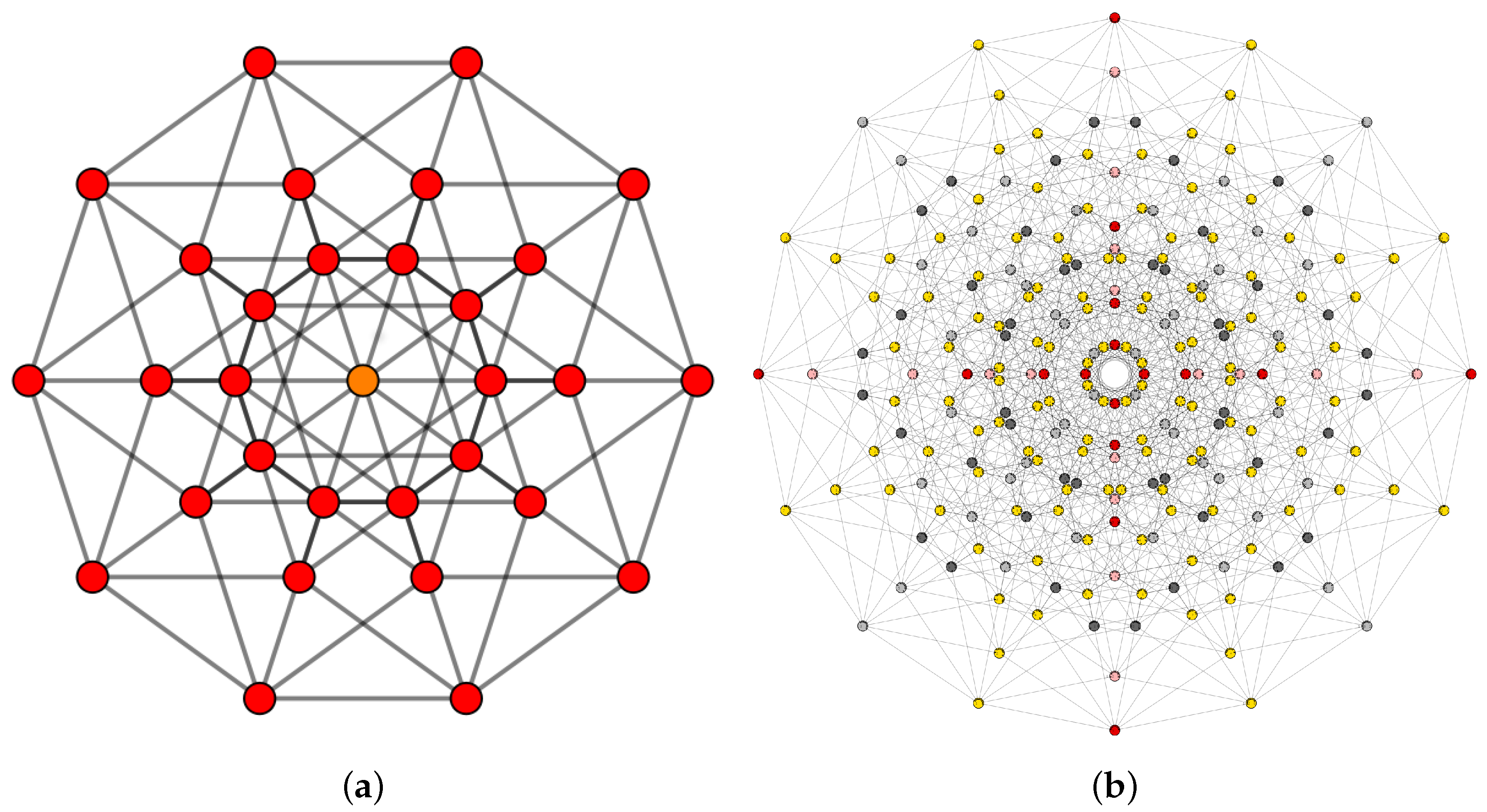
17] projections. However, these methods mainly aim to maintain symmetries of an RP to the highest degree; the resulting images thus only transmit vertex and edge information. Therefore, a major defect of existing projections is that they lack crucial metric or topological data; see the examples illustrated in Figure 1. In fact, using traditional projections, it is difficult to establish their detailed geometric structure. To this end, in [7], we studied the generalized stereographic projection to observe 4D RPs. This method preserves both the metric and topological data of 4D RPs, from which one can identify their general symmetrical structure better.
Compared to 4D RPs [18,19], 5D RPs are more complex and have richer symmetries. In this paper, by generalizing the idea of [7], we study in detail the 2D and 3D stereographic projections of 5D RPs. It is a simple and universal strategy that can be extended to RPs in higher dimensional space. The remainder of this paper is outlined as follows. In Section 2, we briefly introduce the structure of 5D RPs, including the symmetry group, fundamental root system, and an important algorithm that transforms an arbitrary point of R 5 into the fundamental region. Then, in Section 3, we describe the 3D and 2D visualization implementations of 5D RPs. Finally, Section 4 concludes the paper and shows future directions on this subject.

2. Geometrical Features of 5D RPs

In this section, we briefly describe the geometrical features of 5D RPs, including their geometrical structures, group representations, fundamental region systems, and common notations. Moreover, we will present an important algorithm that transforms an arbitrary point of R 5 into a fundamental region symmetrically.
5D RPs are the analogs of regular polytopes in R 4 . Their geometrical structure is precisely specified by the concise Schläfli symbols { p , q , r , s } , where p is the number of sides of each regular polygon, q the number of regular polygons meeting at each vertex in a cell, r the number of regular polyhedra { p , q } meeting along each edge, and s the number of 4D RP { p , q , r } meeting around each 4D face. It is well known that there are only three regular polytopes in R 5 : 5-simplex { 3 , 3 , 3 , 3 } , 5-cube { 4 , 3 , 3 , 3 } , and 5-orthoplex { 3 , 3 , 3 , 4 } .
To understand the Schläfli symbol better, let us take the five-simplex { 3 , 3 , 3 , 3 } as an example. The first three tells us that face { 3 } is an equilateral triangle. The second three shows that there are three { 3 } s meeting at each vertex. Thus we see that { 3 , 3 } is the familiar regular tetrahedron, which is called a cell. The third three means that there are three { 3 , 3 } s meeting along each edge, which forms a 4D RP { 3 , 3 , 3 } , called a facet. Finally, the last three means that 5D { 3 , 3 , 3 , 3 } has three 4D RPs { 3 , 3 , 3 } around each 4D face. In short, the five-simplex { 3 , 3 , 3 , 3 } has in total 6 vertices, 15 edges, 20 equilateral triangles, 15 tetrahedrons, and 6 4D-RPs. The main geometrical features of 5D RPs are summarized in Table 1.
Each 5D RP { p , q , r , s } has a dual RP { s , p , q , r } . They share the same reflection symmetry group, which is usually denoted by [ p , q , r , s ] . The five-simplex { 3 , 3 , 3 , 3 } is self-dual and corresponds to the reflection symmetry group [ 3 , 3 , 3 , 3 ] , which is usually denoted as B 5 . The other two 5D RPs, five-cube { 4 , 3 , 3 , 3 } and five-orthoplex { 3 , 3 , 3 , 4 } , are dual and share the same reflection symmetry group [ 3 , 3 , 3 , 4 ] , called D 5 . B 5 and D 5 have 3840 and 1920 symmetries, respectively.
Group [ p , q , r , s ] is generated by five proper reflections s 1 , s 2 , s 3 , s 4 , s 5 . The abstract representation of group B 5 = [ 3 , 3 , 3 , 3 ] is:
s 1 2 = = s 5 2 = ( s 1 s 2 ) 3 = = ( s 4 s 5 ) 3 = ( s 1 s 3 ) 2 = ( s 2 s 4 ) 2 = ( s 3 s 5 ) 2 = 1 ,
where the last one represents the unit element. The abstract representation of group D 5 = [ 3 , 3 , 3 , 4 ] is:
s 1 2 = = s 5 2 = ( s 1 s 2 ) 3 = ( s 2 s 3 ) 3 = ( s 3 s 4 ) 3 = ( s 3 s 5 ) 3 = ( s 1 s 3 ) 2 = ( s 2 s 4 ) 2 = ( s 4 s 5 ) 2 = 1 .
Assume v is a nonzero normal vector with respect to hyperplane P, then the reflection Π v associated with P is:
Π v ( x ) = x - 2 ( x , v ) ( v , v ) v ,
where ( · , · ) denotes the inner product of vectors. Obviously, Π v ( x ) = x if x P and Π v ( x ) = - x if x P T (the orthogonal space of P). The fundamental root system with respect to [ p , q , r , s ] is a vector set formed by certain vectors so that the associated reflections are precisely generators of [ p , q , r , s ] . In this paper, the fundamental root system associated with [ p , q , r , s ] is denoted by Δ [ p , q , r , s ] = { v 1 , v 2 , v 3 , v 4 , v 5 } . The fundamental root systems of B 5 and D 5 are listed in Table 2 [20].
The fundamental region under group [ p , q , r , s ] is a connected set, whose transformed copies under the action of [ p , q , r , s ] cover the entire space without overlapping except at boundaries [1]. The fundamental region of 5D RP can be elegantly described by the fundamental root system [20]: it is a closed set of points in R 5 satisfying:
D [ p , q , r , s ] = { ξ R 5 | ( ξ , v k ) 0 , v k Δ [ p , q , r , s ] } .
Assume P v i is the hyperplane passing through the origin with normal vector v i ( i = 1 , 2 , . . . , 5 ). Then, geometrically, the fundamental region D [ p , q , r , s ] is a 5D cone surrounded by hyperplanes P v i whose vertex is the origin. Though it is a little bit difficult to imagine the appearance of D [ p , q , r , s ] , the 3D cone is familiar; see a 3D example illustrated in Figure 2.
For x 0 R 5 outside D [ p , q , r , s ] , there is a fast algorithm to transform x 0 symmetrically into the fundamental region D [ p , q , r , s ] . To show how this algorithm works, we first introduce a lemma.
Lemma 1.
Assume v is a nonzero normal vector with respect to the hyperplane P. Points α 0 and α 1 are points on different sides of P, i.e.,
( α 0 , v ) < 0 ( α 1 , v ) > 0 o r ( α 0 , v ) > 0 ( α 1 , v ) < 0
where ( · , · ) denotes the inner product of vectors. Then:
| | Π v ( α 0 ) - α 1 | | 2 < | | α 0 - α 1 | | 2 ,
where Π v is the reflection associated with P and | | · | | 2 is the Euclidean norm.
Proof. 
It is obvious that:
| | Π v ( α 0 ) - α 1 | | 2 2 = | | α 0 - 2 ( α 0 , v ) ( v , v ) v - α 1 | | 2 2 = α 0 - α 1 - 2 ( α 0 , v ) ( v , v ) v , α 0 - α 1 - 2 ( α 0 , v ) ( v , v ) v = α 0 - α 1 , α 0 - α 1 + 4 ( α 0 , v ) ( α 1 , v ) ( v , v ) = | | α 0 - α 1 | | 2 2 + 4 ( α 0 , v ) ( α 1 , v ) ( v , v ) .
By (1), we see ( α 0 , v ) ( α 1 , v ) ( v , v ) < 0 . Thus, we have (2). □
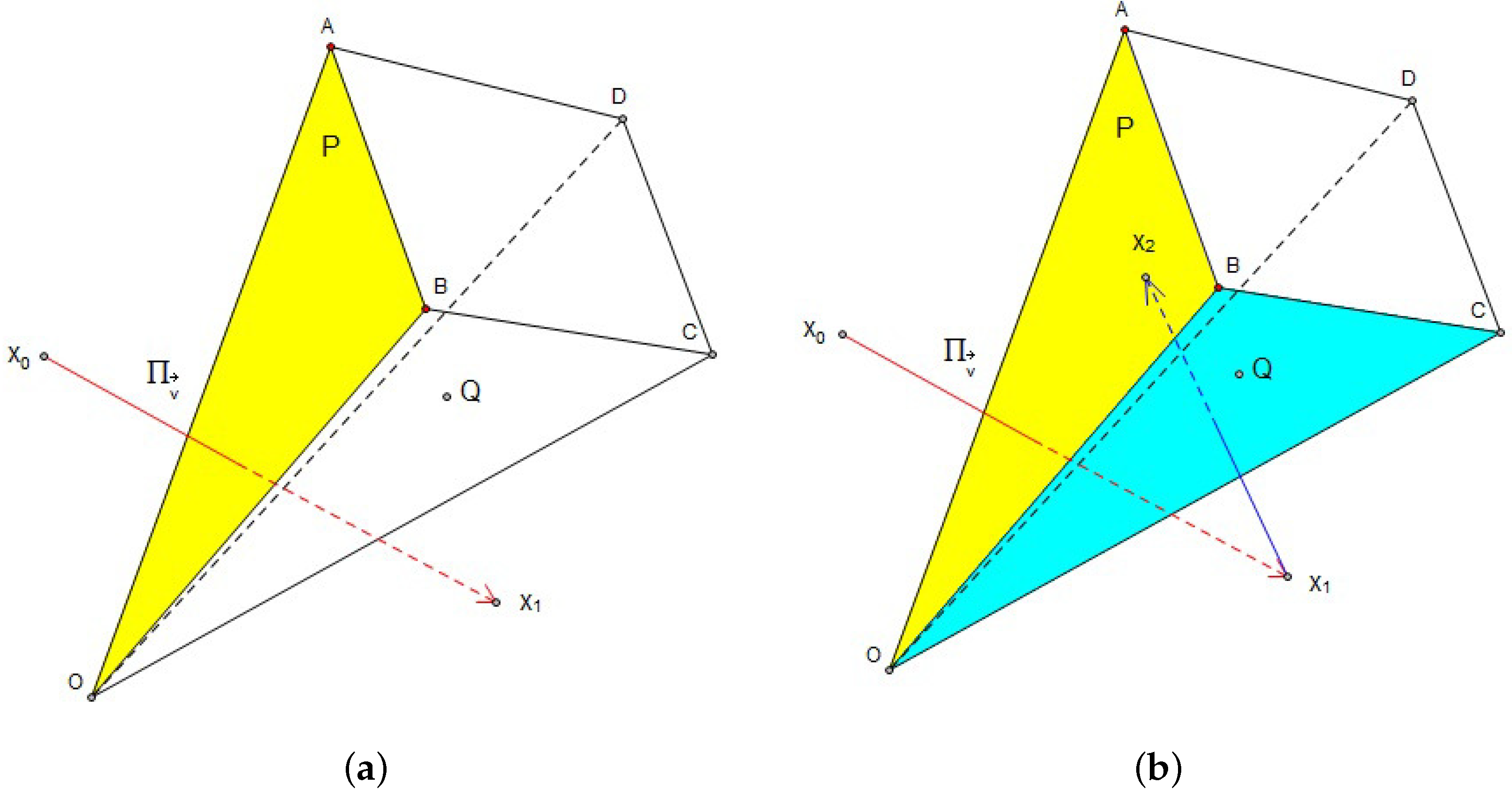
We use a diagram to explain the geometric meaning of Lemma 1. In Figure 2a, assume Q D [ p , q , r , s ] and x 0 D [ p , q , r , s ] are points on different sides of a plane P. Then, x 1 = Π v ( x 0 ) and Q lie on the same side of P. Lemma 1 says that the distance between x 1 and Q is smaller than x 0 and Q. In other words, for two points on the different sides of a plane, the reflection transformation associated with P can shorten their distance.
Theorem 1.
Let D [ p , q , r , s ] be the fundamental region with respect to group [ p , q , r , s ] . For a point x 0 outside D [ p , q , r , s ] , there exists a transformation Γ n [ p , q , r , s ] and a symmetrically-placed point x n such that x n = Γ n ( x 0 ) [ p , q , r , s ] .
Proof. 
Assume Q is an interior point of the fundamental region D [ p , q , r , s ] . For x 0 D [ p , q , r , s ] , recalling the definition of D [ p , q , r , s ] , there must exist a k { 1 , , 5 } so that ( x 0 , v k ) < 0 . In other words, x 0 and Q lie on different sides of the hyperplane P v k ( P v k is the hyperplane passing through the origin with normal vector v k ); denoted by x 1 = Π v k ( x 0 ) . By Lemma 1, we have:
| | Q - Π v k ( x 0 ) | | 2 < | | Q - x 1 | | 2 .
If x 1 D [ p , q , r , s ] , there exists a Π v j so that | | Q - Π v j ( x 1 ) | | 2 < | | Q - x 2 | | 2 , where x 2 = Π v j ( x 1 ) .
Thus, each time a chosen reflection Π v k is employed, the transformed x i = Π v k ( x i - 1 ) will get nearer to Q and eventually fall into D [ p , q , r , s ] . Let n be the reflection times and Γ n be the product of the employed Π v k , then x n = Γ n ( x 0 ) [ p , q , r , s ] . □
Theorem 1 describes an algorithm that transforms points into D [ p , q , r , s ] symmetrically. Figure 2b illustrates an example of how Theorem 1 works. For convenience, we call it the fundamental region algorithm (FRA) and summarize the corresponding pseudocode in Algorithm 1 so that the interested readers can create their own projection patterns. Essentially, it is the kaleidoscope principle in higher dimension Euclidean space [1,2,3].
Algorithm 1 Fundamental region algorithm (FRA).
Input: Point x 0 R 5 and fundamental root system { v 1 , v 2 , v 3 , v 4 , v 5 }
Output: Point x n D [ p , q , r , s ] and reflection number n
1:
Let n = 0
2:
Compute sign: s i g n = 0
3:
for k = 1 –5 do
4:
if ( x 0 , v k ) > 0 then
5:
   s i g n = s i g n + 1
6:
end if
7:
end for
8:
while s i g n < 5 do
9:
n = n + 1
10:
for k = 1 to 5 do
11:
  if ( x n - 1 , v k ) < 0 then
12:
    x n = Π v k ( x n - 1 ) = x n - 1 - 2 ( x n - 1 , v k ) ( v k , v k ) v k
13:
    Π n = Π v k
14:
   Compute sign: s i g n = 0
15:
   for i = 1 to 5 do
16:
    if ( x n , v i ) > 0 then
17:
      s i g n = s i g n + 1
18:
    end if
19:
   end for
20:
   break
21:
  end if
22:
end for
23:
end while
24:
n is the repeated Steps 8–23, then point x n = Γ n ( x 0 ) = Π n × Π n - 1 × × Π 1 ( x 0 ) D [ p , q , r , s ] .

3. Visualizations of 5D RPs from Generalized Stereographic Projection

In this section, we first introduce the generalized stereographic projection. Then, we describe 2D or 3D visualization methods for 5D RPs.
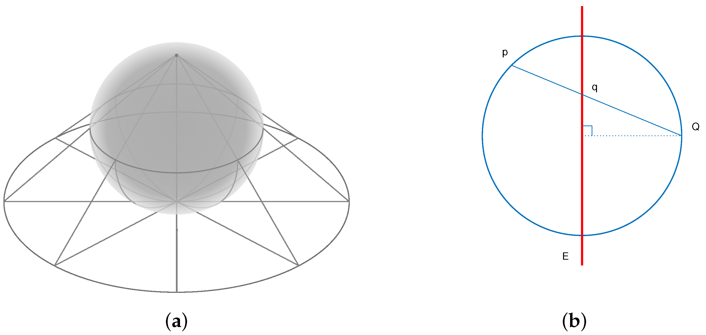
Denote by S n = { ( x 1 , x 2 , . . . , x n + 1 ) R n + 1 | j = 1 n + 1 x j 2 = 1 } the unit sphere and Q = ( 0 , 0 , , 0 , 1 ) S n . Suppose E = { ( x 1 , x 2 , . . . , x n , x n + 1 ) R n + 1 | x n + 1 = 0 } is a hyperplane. Then, the stereographic projection of a point p S n \ { Q } is the intersection point q between line Q p ¯ and E. Figure 3 demonstrates the situation of 2D and 3D stereographic projections. Assume p = ( x 1 , x 2 , , x n + 1 ) S n \ { Q } . According to the stereographic projection, the relation between q and p is:
q = ( X 1 , X 2 , , X n ) = ϕ n ( p ) = 1 1 - x n + 1 ( x 1 , x 2 , , x n ) .
Let:
θ 2 = j = 1 n X j 2 .
Then, the inverse of the stereographic projection is:
p = ( x 1 , x 2 , , x n + 1 ) = ϕ n - 1 ( q ) = 1 θ 2 + 1 2 X 1 , , 2 X n , θ 2 - 1 .
It is easy to check that x 1 2 + x 2 2 + + x n + 1 2 = 1 , which means that the pre-image of ( X 1 , X 2 , , X n ) under projection ϕ n always lies on S n .
For a point ( X 1 , X 2 , X 3 ) R 3 , we can compute the corresponding point ( x 1 , x 2 , x 3 , x 4 , x 5 ) R 5 by using stereographic projection twice, that is:
( x 1 , x 2 , x 3 , x 4 , x 5 ) = r 4 · ϕ 4 - 1 r 3 · ϕ 3 - 1 X 1 , X 2 , X 3 = 1 θ 4 2 + 1 4 X 1 r 3 r 4 θ 3 2 + 1 , 4 X 2 r 3 r 4 θ 3 2 + 1 , 4 X 3 r 3 r 4 θ 3 2 + 1 , 2 r 4 ( θ 3 2 - 1 ) θ 3 2 + 1 , θ 4 2 - 1 = 1 θ 4 2 + 1 · r 3 r 4 θ 3 2 + 1 4 X 1 , 4 X 2 , 4 X 3 , 2 ( θ 3 2 - 1 ) r 3 , ( θ 3 2 + 1 ) ( θ 4 2 - 1 ) r 3 r 4
where:
θ 3 2 = j = 1 3 r 3 2 X j 2 , θ 4 2 = r 4 θ 3 2 + 1 2 j = 1 3 ( 2 r 3 X j ) 2 + ( θ 3 2 - 1 ) 2 ,
and r k is the parameters specifying the radii of ( k + 1 ) -dimensional sphere S k .
Assume N is the number of steps employed in FRA. On average, each point of S 4 will be transformed into the fundamental region D [ p , q , r , s ] of 5D RPs within 10–13 times, a little larger than 4D RPs (8–10 times [8]) and regular polyhedra (4–7 [7]). According to N odd or even, one can use two colors to color a 3D point ( X 1 , X 2 , X 3 ) and obtain a two-color interlaced image of 5D RPs. We next use this scheme to create some projection patterns in R 2 and R 3 .
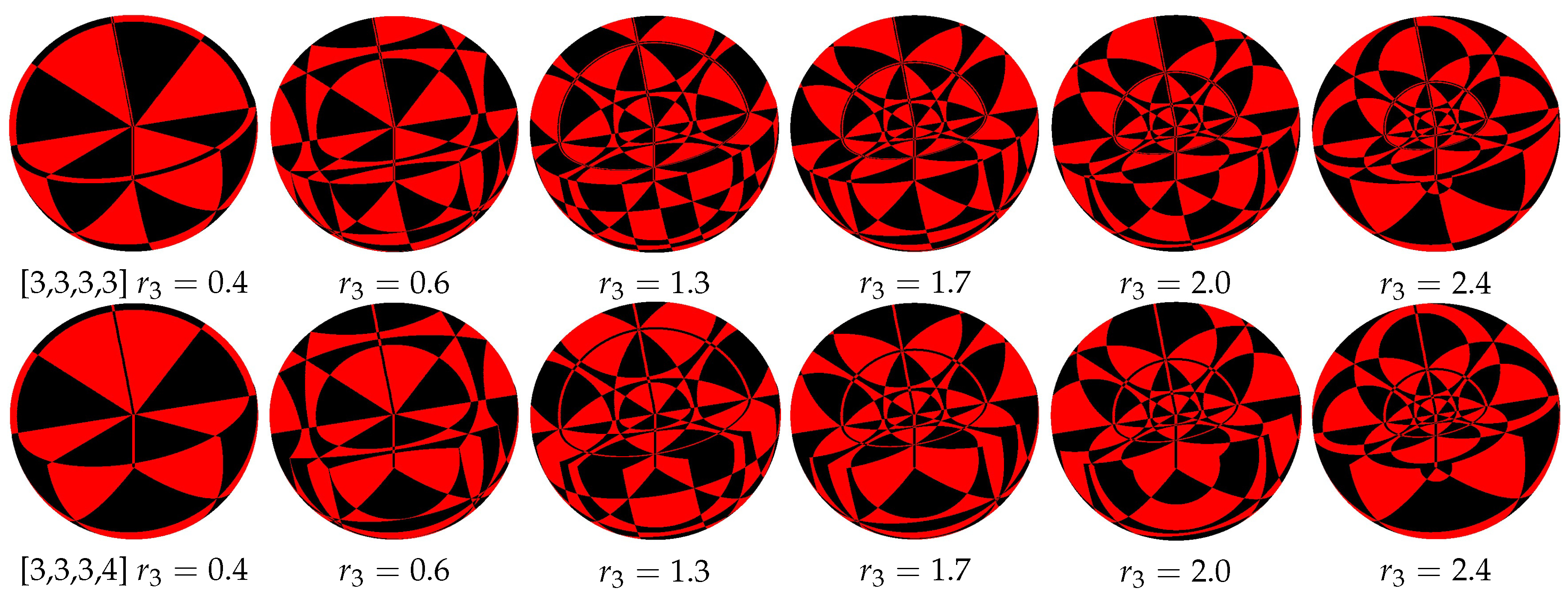
In the first situation, by fixing r 3 = 2 and varying r 4 , Figure 4 shows the sphere projections of 5D RPs. In the second situation, by fixing r 4 = 0.5 and varying r 3 , Figure 5 and Figure 6, respectively, illustrate the sphere projections of B 5 and D 5 . As the order of B 5 is twice that of D 5 , it is easy to see that the projection of B 5 is more complex than D 5 . The value of r 3 can be sensitive to small changes, so in these two images, we have chosen certain values so that the change of projections is relatively obvious. We observe an interesting phenomenon: at first, projections tend to be complex as r 3 increases; however, projections become simpler once r 3 exceeds a certain threshold.
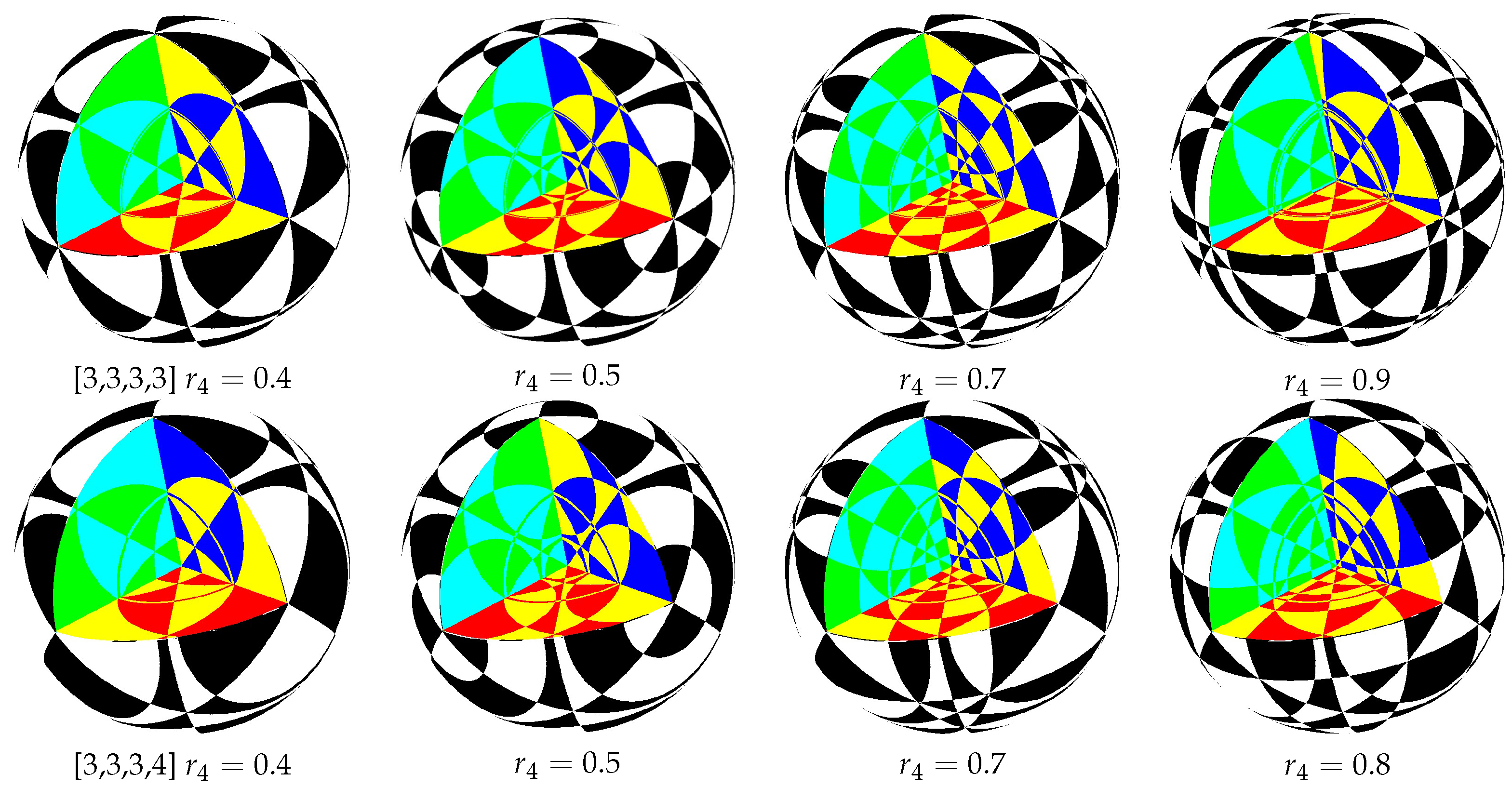
Figure 7 and Figure 8, respectively, display the effect of unit solid sphere projections of 5D RPs, where 1 / 8 and 1 / 4 of the spherical solids are cut off so that they exhibit some inner details. For clarity, several colors are used in the sections.
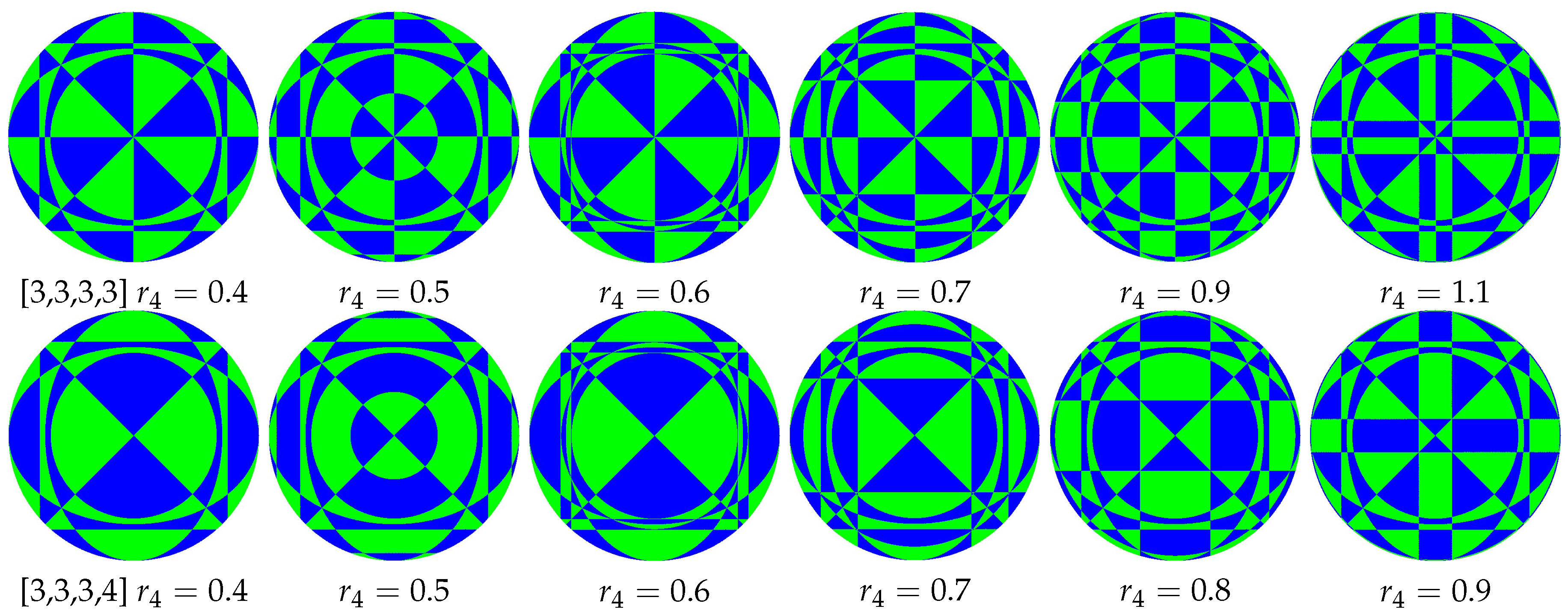
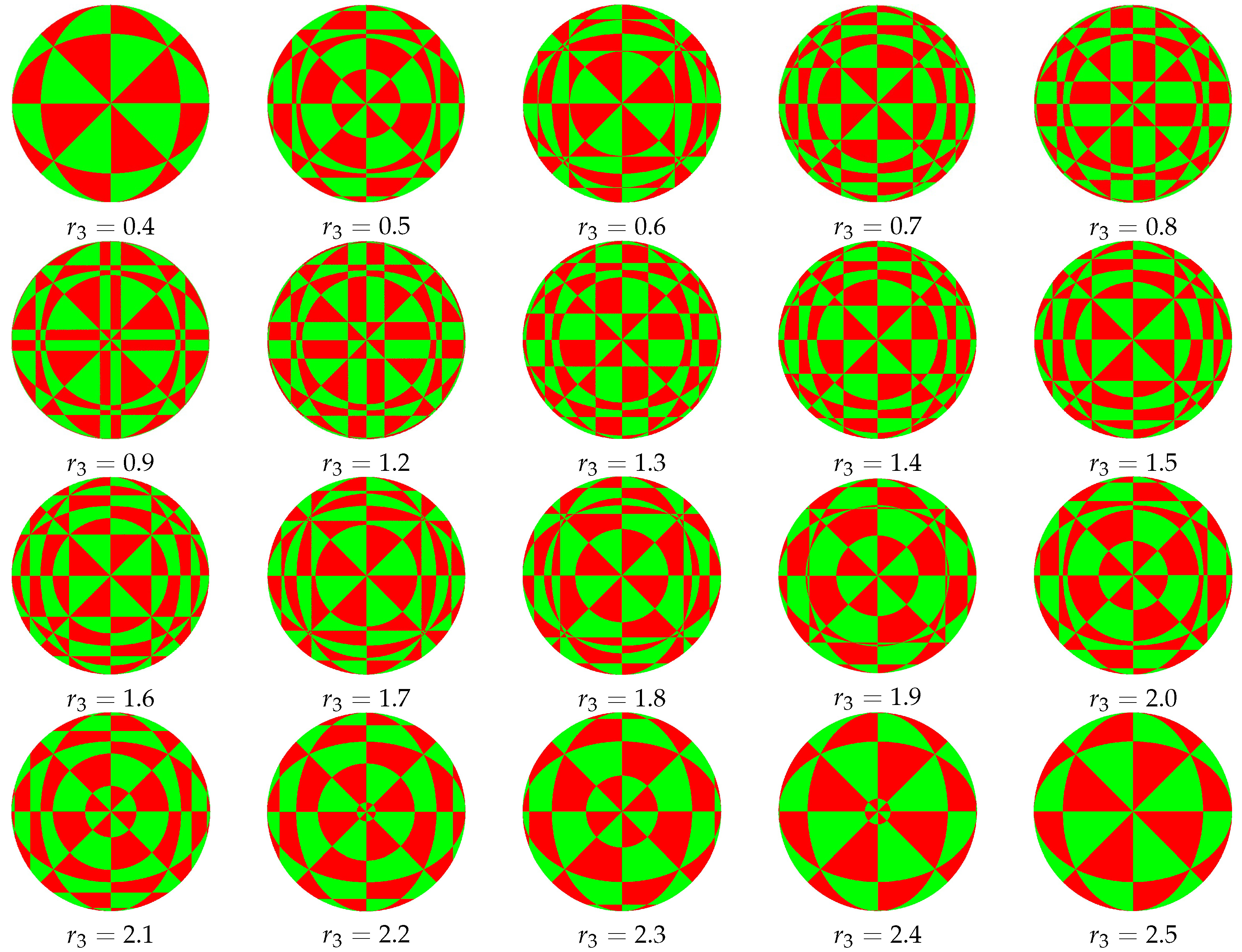
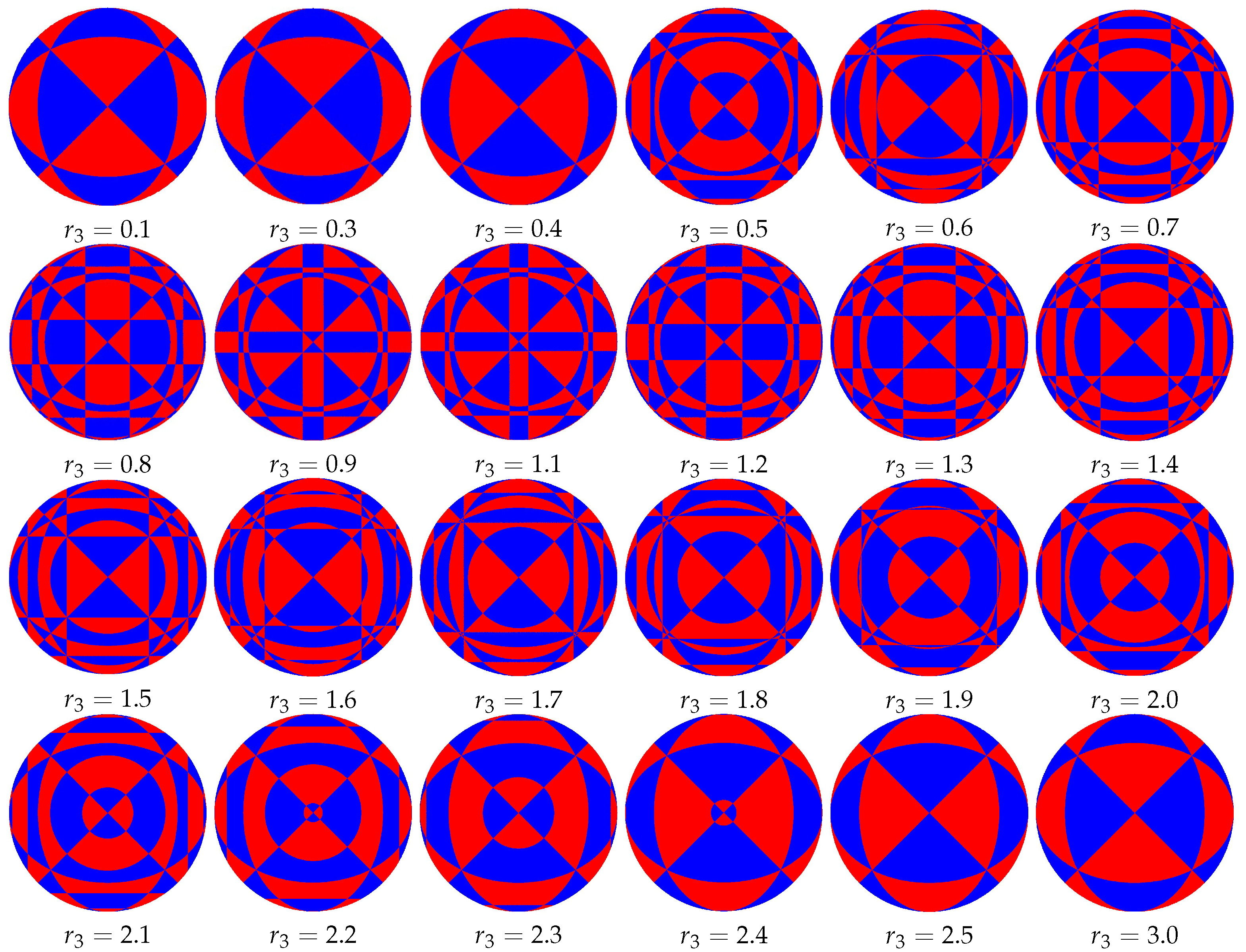
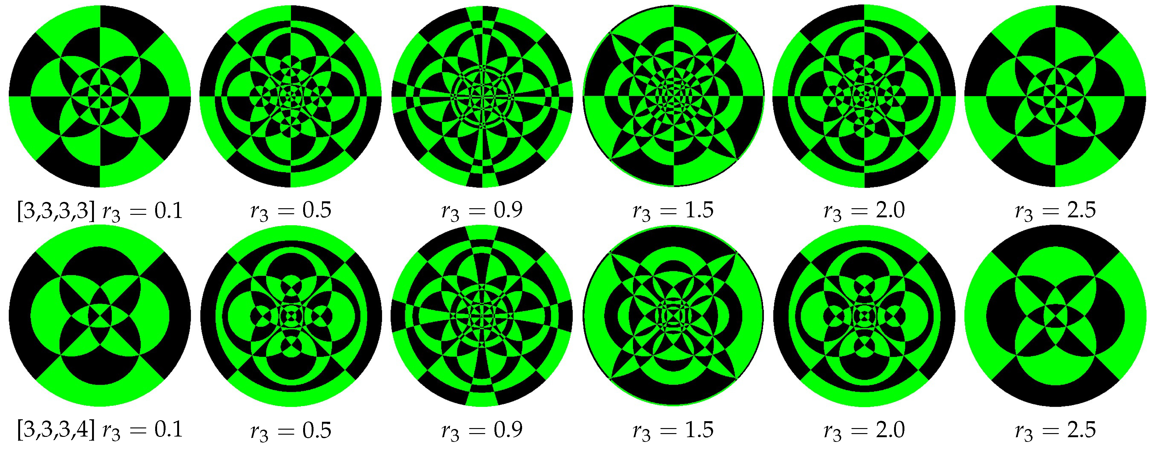
We next consider 2D projections of 5D RPs. For a point ( X 1 , X 2 ) R 2 , we can similarly compute its corresponding point ( x 1 , x 2 , x 3 , x 4 , x 5 ) R 5 by using stereographic projection three times. More precisely,
( x 1 , x 2 , x 3 , x 4 , x 5 ) = r 4 · ϕ 4 - 1 r 3 · ϕ 3 - 1 r 2 · ϕ 2 - 1 X 1 , X 2 = r 3 r 4 ( θ 2 2 + 1 ) ( θ 3 2 + 1 ) ( θ 4 2 + 1 ) 8 r 2 X 1 , 8 r 2 X 2 , 4 ( θ 2 2 - 1 ) , 2 ( θ 2 2 + 1 ) ( θ 3 2 - 1 ) r 3 , ( θ 2 2 + 1 ) ( θ 3 2 + 1 ) ( θ 4 2 - 1 ) r 3 r 4 ,
where:
θ 2 2 = j = 1 2 r 2 2 X j 2 , θ 3 2 = r 3 θ 2 2 + 1 2 j = 1 2 ( 2 r 2 X j ) 2 + ( θ 2 2 - 1 ) 2 , θ 4 2 = r 4 θ 3 2 + 1 · r 3 θ 2 2 + 1 2 j = 1 2 ( 4 r 2 X j ) 2 + 2 ( θ 2 2 - 1 ) 2 + ( θ 2 2 + 1 ) ( θ 3 2 - 1 ) r 3 2
and r k are parameters specifying the radii of the ( k + 1 ) -dimensional sphere. By fixing r 2 = 1 and varying r 3 and r 4 separately, Figure 9 and Figure 10 demonstrate the 2D projections of 5D RPs. Again, we see, as r 3 or r 4 is increasing, those projections will first change from simple to complex and then back to simple.

4. Conclusions

Based on the geometrical meaning of RPs, this paper presents a convenient strategy to visualize 5D RPs, which could be extended to treat n-dimensional RPs ( n > 5 ). We first introduced their structure, Schläfli symbol, group representation, and fundamental root system. Then, we proved the generalized kaleidoscope principle that transforms an arbitrary point of R 5 into a fundamental region symmetrically. For convenience, the kaleidoscope principle was summarized in Algorithm 1. Using the algorithm, we finally presented the visualization implementations of 5D RPs.
The foundations of RPs were laid by the Greeks over two thousand years ago. Over the past two hundred years, many excellent mathematicians around the world have made a systematic, extensive, and in-depth study of RPs. In the bibliography of the classic Regular Polytopes, H.S.M.Coxeter listed the name of 110 mathematicians: 30 German, 27 British, 12 American, 11 French, 7 Dutch, 8 Swiss, 4 Italian, 2 Austrian, 2 Hungarian, 2 Polish, 2 Russian, 1 Norwegian, 1 Danish, and 1 Belgian. He commented that “the chief reason for studying regular polyhedra is still the same as in the time of the Pythagoreans, namely, that their symmetrical shapes appeal to one’s artistic sense”. The first edition of the Regular Polytopes was published in 1948, but there has been no major change in the following. Due to the early completion of the book—the computer had just been born–much of the visualization study of RPs is not discussed in depth.
The fundamental root system and fundamental region, which in practice helped H.S.M. Coxeter to complete the classification of irreducible reflective groups [20], constituted the core theoretical tool of this study. In this paper, we saw that those tools can be used easily to create infinite exotic spherical tilings. Generally speaking, the construction of spherical tilings is not easy. For the past decade, many very complex methods have been reported to construct spherical tilings; see [21,22] and the references therein. In the future, we plan to investigate the relation between Algorithm 1 and the associated spherical tilings, which aims to present a simple and efficient approach to construct rich spherical tilings.

Author Contributions

X.W. conceived the framework and structured the whole paper; T.Y. performed the experiments and wrote the paper; K.C. and K.G. checked the results; P.O., X.W. and T.Y. completed the revision of the article.

Funding

This research received no external funding.

Acknowledgments

We thank the anonymous reviewers for their helpful comments. This work was supported by the Natural Science Foundation of China (Nos. 11461035 and 11761038) and the Science and Technology Plan Project of Jiangxi Provincial Education Department (Nos. GJJ160749 and GJJ160758).

Conflicts of Interest

The authors declare no conflict of interest.

References

  1. Coxeter, H.S.M. Regular Polytopes; Dover: New York, NY, USA, 1973. [Google Scholar]
  2. Coxeter, H.S.M. Regular Complex Polytopes; Cambridge University Press: London, UK, 1991. [Google Scholar]
  3. McMullen, P.; Schulte, E. Abstract Regular Polytopes; Cambridge University Press: Cambridge, UK, 2002. [Google Scholar]
  4. Grünbaum, B.; Shephard, G.C. Tilings and Patterns; CERN Document Server: New York, NY, Freeman, 1987. [Google Scholar]
  5. Conway, J.H.; Burgiel, H.; Goodman-Strauss, C. The Symmetries of Things; A K Peters Press: Natick, MA, USA, 2008. [Google Scholar]
  6. Kaplan, C.S. Computer Graphics and Geometric Ornamental Design. Ph.D. Thesis, University of Washington, Washington, DC, USA, 2002. [Google Scholar]
  7. Ouyang, P.C.; Wang, L.; Yu, T.; Huang, X. Aesthetic Patterns with Symmetries of the Regular Polyhedron. Symmetry 2017, 9, 21. [Google Scholar] [CrossRef]
  8. Ouyang, P.C.; Wang, X.C.; Zhao, Y.M. Beautiful Math, Part 6: Visualizing 4D Regular Polytopes Using the Kaleidoscope Principle. IEEE Comput. Graph. Appl. 2017, 37, 92–97. [Google Scholar] [CrossRef] [PubMed]
  9. Horne, C.E. Geometric Symmetry in Patterns and Tilings; Woodhead Publishing: Sawston, UK, 2000. [Google Scholar]
  10. Stewart, I.; Golubitsky, M. Fearful Symmetry: Is God a Geometer? Dover Publications: Mineola, NY, USA, 2011. [Google Scholar]
  11. Armstrong, V.E. Groups and Symmetry; Springer: New York, NY, USA, 1987. [Google Scholar]
  12. Stevens, P.S. Handbook of Regular Patterns; MIT Press: Cambridge, MA, USA, 1981. [Google Scholar]
  13. Hahn, T. International Tables for Crystallography; Kluwer Academic Publishers: Boston, MA, USA, 1996. [Google Scholar]
  14. Suck, J.B.; Schreiber, M.; Haussler, P. Quasicrystals: An Introduction to Structure; Springer: Berlin, Germany, 2002. [Google Scholar]
  15. Park, H.G. A Workshop on N-regular Polygon Torus Using 4D Frame. In Proceedings of Bridges 2013: Mathematics, Music, Art, Architecture, Culture; Tessellations Publishing: Enschede, The Netherlands, 2013; pp. 597–600. [Google Scholar]
  16. Séquin, C.H.; Lanier, J. Hyperseeing the Regular Hendecachoron. In Proceedings of the ISAMA Conferences, College Station, TX, USA, 18–21 May 2007; pp. 159–166. [Google Scholar]
  17. Reiter, C.A. Chaotic Attractors Exhibiting Quasicrystalline Structure. Comput. Graph. 2008, 3, 511–517. [Google Scholar] [CrossRef]
  18. Ramírez, A.A.; Aguila, R.P. Presenting Methods for Unraveling the First Two Regular 4D Polytopes (4D Simplex and the Hypercube). In Proceedings of the International Symposium on Cyber Worlds, Tokyo, Japan, 6–8 November 2002. [Google Scholar]
  19. Koca, M.; Koca, N.O.; Al-Ajmi, M. 4D-Polytopes and Their Dual Polytopes of the Coxeter Group W(A4) Represented by Quaternions. Int. J. Geom. Methods Mod. Phys. 2012, 9, 1250035. [Google Scholar] [CrossRef]
  20. Humphreys, J.E. Reflection Groups and Coxeter Groups; Cambridge University Press: Cambridge, UK, 1990. [Google Scholar]
  21. Breda, A.M.; Ribeiro, P.S. Spherical F-Tilings by Two Non Congruent Classes of Isosceles Triangles-I. Math. Commun. 2012, 17, 127–149. [Google Scholar]
  22. Avelino, C.P.; Santos, A.F. Spherical F-tilings by Scalene Triangles and Isosceles Trapezoids, II. Acta Math. Sin. 2012, 28, 1013–1032. [Google Scholar] [CrossRef]
Figure 1. Traditional projections only show vertex and edge information. They lack crucial metric or topological data, so that one can hardly understand the real structure of regular polytopes (RPs). (a) Orthographic projection of a 5D hypercube { 4 , 3 , 3 , 3 } . (b) Orthographic projection of an 8D hypercube { 4 , 3 , 3 , 3 , 3 , 3 , 3 } .
Symmetry 11 00391 g001
Figure 2. (a) Let Q D [ p , q , r , s ] and x 0 D [ p , q , r , s ] be points on the different sides of plane P. Then, x 1 = Π v ( x 0 ) and Q will lie on the same side of P, and the distance between x 1 and Q is smaller than x 0 and Q. (b) A 3D schematic illustration that shows how Theorem 2.2 transforms x 0 D [ p , q , r , s ] into D [ p , q , r , s ] symmetrically. In this case, Q D [ p , q , r , s ] and x 0 D [ p , q , r , s ] . Point x 0 is first reflected about plane O A B to point x 1 D [ p , q , r , s ] . Then, point x 1 is reflected about plane O B C to point x 2 D [ p , q , r , s ] .
Symmetry 11 00391 g002
Figure 3. (a) Case of the stereographic projection in R 3 . (b) Case of the stereographic projection in R 2 .
Symmetry 11 00391 g003
Figure 4. Using Projection (7), symmetrical patterns of 5D RPs on the unit sphere with r 3 = 2 .
Symmetry 11 00391 g004
Figure 5. Using Projection (7), symmetrical patterns of [3,3,3,3] on the unit sphere with r 4 = 0 . 5 .
Symmetry 11 00391 g005
Figure 6. Using Projection (7), symmetrical patterns of [3,3,3,4] on the unit sphere with r 4 = 0.5.
Symmetry 11 00391 g006
Figure 7. Using Projection (7), unit solid sphere projections of 5D RPs with radius r 3 = 2 .
Symmetry 11 00391 g007
Figure 8. Using Projection (7), unit solid sphere projections of 5D RPs with r 4 = 0 . 5 .
Symmetry 11 00391 g008
Figure 9. Using Projection (8), symmetrical patterns of 5D RPs on the unit disc with r 3 = 0.5.
Symmetry 11 00391 g009
Figure 10. Using Projection (8), symmetrical patterns of 5D RPs on the unit disc with r 4 = 0 . 5 .
Symmetry 11 00391 g010
Table 1. Geometrical features of 5D regular polytopes.
NameSchläfli symbol
{ p , q , r , s }
Facets
{ p , q , r }
Cells
{ p , q }
Faces
{ p }
EdgesVerticesFace
Figure
{ s }
Edge
Figure
{ r , s }
Vertex
Figure
{ q , r , s }
B 5 5-simplex
(Hexateron)
{3, 3, 3, 3}6
{ 3 , 3 , 3 }
15
{ 3 , 3 }
20
{ 3 }
156 { 3 } { 3 , 3 } { 3 , 3 , 3 }
D 5 5-cube
(Penteract)
{4, 3, 3, 3}10
{ 4 , 3 , 3 }
40
{ 4 , 3 }
80
{ 4 }
8032 { 3 } { 3 , 3 } { 3 , 3 , 3 }
5-orthoplex
(Pentacross)
{3, 3, 3, 4}32
{ 3 , 3 , 3 }
80
{ 3 , 3 }
80
{ 3 }
4010 { 4 } { 3 , 4 } { 3 , 3 , 4 }
Table 2. Fundamental root system with respect to symmetry group [ p , q , r , s ] .
NameSchl a ¨ fli Symbol
{ p , q , r , s }
Reflection Symmetry Group
[ p , q , r , s ]
Fundamental Root System
Δ [ p , q , r , s ] = { v 1 , v 2 , v 3 , v 4 , v 5 }
Order of
[ p , q , r , s ]
B 5 5-simplex
(Hexateron)
{3, 3, 3, 3}[3, 3, 3, 3](1, -1, 0, 0,0), (0, 1, -1, 0, 0),
(0, 0, 1, -1, 0), (0, 0, 0, 1,-1),
(0, 0, 0, 0, 1)
3840
D 5 5-cube
(Penteract)
{4, 3, 3, 3}[3, 3, 3, 4](1, -1, 0, 0,0), (0, 1, -1, 0, 0),
(0, 0, 1,-1, 0), (0, 0, 0, 1,-1),
(0, 0, 0, 1, 1)
1920
5-orthoplex
(Pentacross)
{3, 3, 3, 4}

