Abstract
Information about college students’ social networks plays a pivotal role in college students’ mental health monitoring and student management. While there have been many studies to infer social networks by data mining, the mining of college students’ social networks lacks consideration of homophily. College students’ social behaviors show significant homophily in the aspect of major and grade. Consequently, the inferred inter-major and inter-grade social ties will be erroneously omitted without considering such an effect. In this work, we aimed to increase the fidelity of the extracted networks by alleviating the homophily effect. To achieve this goal, we propose a method that combines the sliding time-window method with the hierarchical encounter model based on association rules. Specifically, we first calculated the counts of spatial–temporal co-occurrences of each student pair. The co-occurrences were acquired by the sliding time-window method, which takes advantage of the symmetry of the social ties. We then applied the hierarchical encounter model based on association rules to extract social networks by layer. Furthermore, we propose an adaptive method to set co-occurrence thresholds. Results suggested that our model infers the social networks of students with better fidelity, with the proportion of extracted inter-major social ties in entire social ties increasing from 0.89% to 5.45% and the proportion of inter-grade social ties rising from 0.92% to 4.65%.
1. Introduction
Modern society is full of competition and cooperation. Social networks connect everyone, and interpersonal skills have become one of the most important metrics to measure one’s talent. In daily life, individuals’ interpersonal behaviors reflect their mental health status. College students (mostly aged between 18 and 24) with psychological disorders, such as anxiety and depression, usually suffer from an interpersonal disorder at the same time [1,2]. The lack of social ties also poses a serious threat to college students’ physical and mental development. Students who lack social connection to others have increased failure experience. They might gradually lose self-confidence and become susceptible to psychological disorders [3,4,5]. Therefore, for better education and management of college students, it is important to know college students’ social ties.
At present, using users’ daily behavior data to mine their social ties has attracted wide attention. Spatiotemporal data, such as those obtained via GPS and cellular networks, are frequently used to extract geographical similarity and social ties between users, e.g., [6,7]. The strength of such ties can be determined based on users’ spatiotemporal co-occurrences, where co-occurrence can be counted using a fixed time slicing method [8]. There are also approaches that use the trajectory of a user’s location data, such as in References [9,10,11]. As such, data are clustered and the accuracy of the prediction can be enhanced.
However, the mining of college students’ social networks is not so well-researched. In college students’ social network mining, one potentially useful information source is the student ID card. With the development of digital and informational campuses, most Chinese universities have established student ID card systems [12,13,14,15]. Student ID cards record students’ daily behaviors, including students’ dining, shopping, book borrowing, library access history, and other data. There are several studies inferring college social networks from the student ID card records. Yao et al. [16] used the consecutive check-in records of each student pair to infer the students’ social network. Liu et al. [17] used the students’ dining transaction data and employed a fixed time slicing method. In the latter, they sliced the time into 5-min slots and if two students appeared in the same slot, then one co-occurrence was counted. Based on the co-occurrence data, they inferred the students’ social networks. The networks were further distilled with a hypothesis test.
Current data mining studies of college students’ social networks lack consideration of the following three issues.
Firstly, although the fixed time slicing method from Reference [17] shows high computational efficiency, transaction data may be sliced into different time slots so that some co-occurrences may get lost.
Secondly, empirical evidence shows that contact between similar people occurs at a higher rate than among dissimilar people. This feature is commonly defined as homophily [18]. Homophily mainly arises from two mechanisms, namely choice homophily and induced homophily [19]. Induced homophily is a passive effect. It arises from the homogeneity of structural opportunities for interaction. Choice homophily is a higher level of homophily. It is mainly a consequence of active choices of individuals. Choice homophily also brings in the social ties that we are interested in. Therefore, in this work, we only considered the alleviation of induced homophily. In the field of education, student social networks also have inherent homophily in terms of race, gender, grade, age, region, and major, among which major homophily and grade homophily are the most significant [20,21,22,23,24,25,26]. Students from the same major and grade have a higher probability of co-occurrence due to similar behaviors resulting from the same courses, examination times, and residence locations. We define inter-(intra-)major or inter-(intra-)grade behaviors as inter-(intra-)group behaviors. Students in different groups are less likely to co-occur even if they have social ties. By ignoring homophily, current models lose fidelity in mining the social network, especially in the inter-group social ties.
Lastly, current models lack a theoretical rationale for setting thresholds for the count of co-occurrences that must take place before a social tie is inferred.
For the above issues, we proposed a hierarchical encounter model based on association analysis [27,28] for inferring college student social networks using the spatial–temporal data recoded by the student ID card. Similar to the approach presented in Reference [8], we used spatiotemporal co-occurrence for inferring the strength of social ties. In this work, one co-occurrence means that two students check in at the same location within a short time period. We used a sliding time-window method to calculate the number of co-occurrences. To combat the homophily effect, we propose a hierarchical encounter model, with which we can mine the intra-group and inter-group social ties separately. The difficulty of setting the co-occurrence threshold was tackled with an adaptive method that varied the threshold for each individual.
This paper is organized as follows. Section 3 provides a description of the dataset used to illustrate the results of the procedure. Then we introduce the sliding time-window approach, and the hierarchical encounter model based on association rules. In Section 5, We discussed that the effectiveness of our method. The last section discusses some limitations of the method and directions for future research.
2. Ethics Statement
This study complies with the guidelines of the 1975 Declaration of Helsinki. This study has been approved by the Institutional Review Board (IRB) from Central China Normal University (CCNU). Our study involves the data of 662 students, so it is hard to get informed consent from every student. Fortunately, in most Chinese university including CCNU, for students from every one to two majors, a grade counselor is assigned to supervise the students. Each major is divided into classes and each class is monitored by a class adviser. Our study was approved by the head of college, all the grade counselors, and all the class advisers. In addition, to protect the privacy of students, all data were anonymized by encrypting student IDs. All subsequent calculations were performed on anonymous data.
3. Data Collection and Data Description
In this paper, we used the subset of the data from Reference [17], which include the check-in data at the food courts and the supermarkets of 662 undergraduate students of the College of Physical Science and Technology (CPST), CCNU. These data are recorded by the student ID card system. We considered 17 check-in locations. When students intend to have their meals or shop at these 17 locations, they can swipe their student ID card at the card scanners to complete the transaction. The scanners will record the student’s transaction information, including the student ID, location, time, money, and item. The scanners will then upload the transaction information to the database of the card system. Through accessing the database, we downloaded the transaction data. The raw data contain all the information we just mentioned, but we only used the student ID, the location, and the time information. We processed the raw data by numbering the student ID and location date and re-formatting the time data.
In fact, there is more than one scanner in each food court or supermarket. We assumed that each food court or supermarket only has one scanner so that a co-occurrence will be recorded if two students check in simultaneously in the same location, even if they use two different scanners. We used to represent the check-in dataset, where is the z-th check-in record and is the total check-in number. Samples of the dataset are tabulated in Table 1, where one row refers to one check-in record . It means student has one check-in event at location at time . represents a student entity, where N is the total number of students. For any student i, it is possible for multiple z to satisfy . represents the location with the total number of locations. is the timestamp for event (the total seconds since 1 January 2014). For example, the first row in Table 1 refers to a check-in for a student whose ID is 153 at location 1 at 1,008,798 s after 1 January 2014.

Table 1.
Examples of check-in data.
We also gathered some personal information of students, including grade, major, gender, and residence location.
4. Mining of the Social Network
To mine the social network, our method mainly consists of two parts, namely the co-occurrence data acquisition, and the hierarchical encounter model based on association rules. Details of the method are introduced in the following sections.
4.1. Co-Occurrence Acquisition
The first step in mining the students’ social network is to obtain the co-occurrence data. In this section, we give our definition of the co-occurrence and compare two co-occurrence acquisition methods, the fixed time slicing method and the sliding window method.
4.1.1. Co-Occurrence and Its Definition
To infer the social network, we first obtained the co-occurrence dataset between any student pair, which reads:
where i and j are the indices of students and is the count of the co-occurrence between students i and j.
Consider the check-in data of location l, where and is the total number of the check-in data in the location l. The time sorted version of is , where . The co-occurrence count is calculated by:
4.1.2. The Fixed Time Slicing Method
In the fixed time slicing method, time is sliced into consecutive, non-overlapping time slots with equal length [17]. In the above equation, is expressed as:
For two students, if they check in during one time slot at location l, then it is considered as one co-occurrence between these students. However, if they check in within time at location l, but in two different time slots, no co-occurrence will be counted. For example, the time interval between the timestamps and , for event and event , is less than , but the events are in different time slots. Therefore, the fixed time slicing method will erroneously omit this co-occurrence.
4.1.3. The Sliding Time-Window Method
An alternative to the fixed time slicing method is the sliding time-window method. In the latter method, the summation term is calculated as:
with being the fixed time interval. If student i checks in at time and student j checks in at time during one time slot at location l, then it is considered as one co-occurrence. Moreover, there are two special cases when only one co-occurrence will be recorded even if there are multiple co-occurrence. The cases are illustrated in Figure 1. For any student pair, at most one co-occurrence will be recorded in one time-window, and one recorded co-occurrence will not be recorded again in the next time-window.

Figure 1.
Two special cases in the sliding time-window method, where (a) one student labeled with i checks in multiple times in one time-window and (b) the same two check-in records of two students labeled with j and k appear in two successive time-windows.
The selection of the starting point and step size in the sliding time-window is crucial. We take the first time point as the starting point and set a variable step size , which is given by:
Algorithm 1 shows the steps to acquire co-occurrence data using the sliding time-window method. In this method, the window slides from to in each iteration where . For example, records and are within ; student and student are counted as one co-occurrence if and do not refer to the identical student. Note that if one student has multiple check-in records within , it is treated as one effective check-in record. As a result, the effect of the consecutive check-in of one student is mitigated. Table 2 gives samples of the co-occurrence, where the first row means that student 53 and student 57 had 120 co-occurrences.
| Algorithm 1: Acquiring co-occurrence data using sliding time-window method |
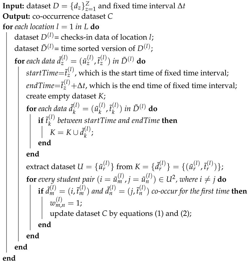 |

Table 2.
Examples of the time of co-occurrence.
4.2. The Hierarchical Encounter Model Based on Association Rules
Having acquired the co-occurrence data, the hierarchical encounter model based on association rules was then used to extract the social ties data:
with being the level of the association of students i and j.
4.2.1. The Hierarchical Encounter Model
College students’ social networks have significant homophily—intra-group students have larger co-occurrence counts, while inter-group students have smaller co-occurrence counts even if they have social ties. In References [16,17], it is assumed that all students are mutually independent and the homophily effect is ignored. Under this assumption, inter-group social ties are buried. Therefore, we propose the hierarchical encounter model to mine the social ties of inter-group students and those of intra-group students separately.
This model is illustrated in Figure 2. It is divided into four levels according to major, college, and grade. Here we use the major homophily as an example, as other types of homophily follow the same steps. For a student, this model mines the intra-major social ties at the first level, and then inter-major social ties at the second level. Detailed steps for the model can be found in Algorithm 2. The social ties of students between college within a university or between grades can be mined using the same method.
| Algorithm 2: The hierarchical encounter model |
| Input: dataset of students from a specific major , dataset of students from a other major , thresholds , and Output: social ties dataset for any student pair R determine ’s frequent itemset by Algorithm 3 using dataset ; calculate by Algorithm 4; determine ’s frequent itemset by Algorithm 3 using dataset and ; calculate by Algorithm 4; calculate social ties dataset using ; |
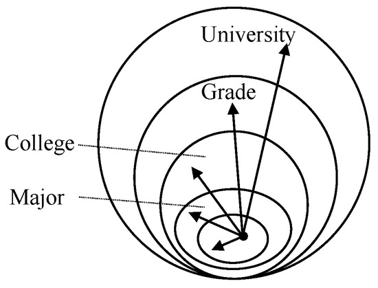
Figure 2.
The hierarchical encounter model. The arrows here represent the statistical process across different levels.
4.2.2. Social Ties Mining With Association Analysis
Based on the co-occurrence data, it is common to use a hypothesis test or a shuffling test to decide how many co-occurrences a pair must have before they are said to be friends [29,30]. The problem is that both approaches require the assumption that student co-occurrences are mutually independent, which is hard to reconcile with the homophily effect. Our main idea is that the co-occurrence count of two students is proportional to the probability that these two students are friends. Therefore, we used association rules to further extract the social ties from the co-occurrence data. Specifically, we calculated the support and confidence to find the association rules, i.e., to find students with strong correlation (social ties) by analyzing the association of each student pair.
For mining intra-major social ties, we used traditional association analysis, which mines association rules in the form of . A social tie from student i to student j exists if the association rule from student i to student j exists. We defined support and confidence of the check-in data as:
and:
respectively, with the total number of the check-ins for student i, the number of co-occurrences of student i and student j, and Z the total number of check-ins in the entire dataset. Support and confidence describe the frequency of the co-occurrence of student i and student j relative to the total number of check-ins in the entire dataset, and student i’s check-in record, respectively. Confidence can be used to represent level of association of student i and student j.
For mining inter-major social ties, we propose the “quasi-association analysis” method. While traditional association analysis can be used to mine rules in the form of and also rules in the form of , quasi-association analysis divides student set U into two separate subsets A and B and mines the association rules in the form of .
Support and confidence are important metrics in association analysis. Association rules with low support might come from random co-occurrence and are usually meaningless. It is common to use a support threshold to sift out those meaningless items and to keep the frequent items. For a certain rule , higher confidence means a larger probability that j appears in the event related to i. The confidence threshold is commonly used to extract high confidence items from frequent items, which are the students’ social ties. Support and confidence thresholds are usually set by users or experts in the traditional approach and are usually fixed [31,32]. However, in mining the college students’ social network, different students have different check-in data numbers. It is therefore unreasonable to use the same threshold for every student. This motivated an adaptive threshold determination approach.
4.2.3. Threshold Determination
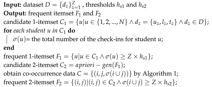
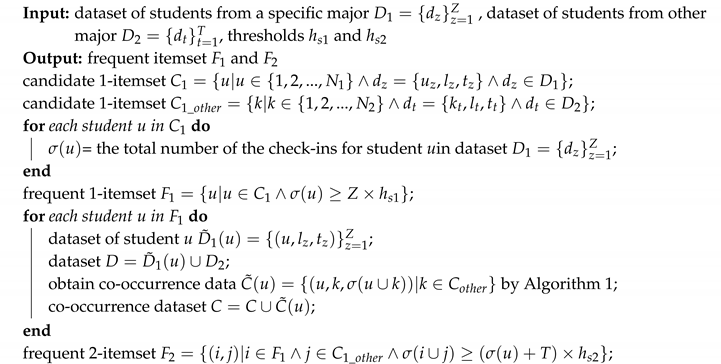
There are three thresholds in this paper, namely , , and , among which and are the support thresholds with used to sift out the students with small numbers of check-ins—it is hard to mine the social ties of students who seldom use the ID card. Threshold is designed to delete pairs of students with very small numbers of co-occurrences. If the co-occurrence of two students is less than , then these two students are considered as entirely uncorrelated. There exists a trade-off between computation complexity and fidelity—a smaller threshold leads to identification of more social networks at the cost of more computation. Algorithms 3 and 4 illustrate steps for determining frequent itemset for students from a specific major and that from other majors through support thresholds and , respectively.
| Algorithm 3: Determining frequent itemset for students from a specific major |
 |
| Algorithm 4: Determining frequent itemset for students from other majors |
 |
The last threshold, , is the confidence threshold. It is used to extract rules with high confidence. Taking student i as an example, let be the result sorting the entire co-occurrence between student i and others in descending order. Figure 3 is the plot of , where the x-axis is the index k while the y-axis is the number of co-occurrences . Figure 3a,b is the co-occurrence of the intra-major students and of the inter-major students, respectively. In both the intra-major and the inter-major case, there exist apparent inflection points in the figures. There are only a few students having large co-occurrence counts with student i, with a large count being one that is higher than the count at the inflection point. We considered these students to have social ties with student i. Most students have small co-occurrence counts with student i, and we considered these co-occurrences to be the result of randomness. Figure 3 provides theoretical fundamentals for the determination of the threshold.
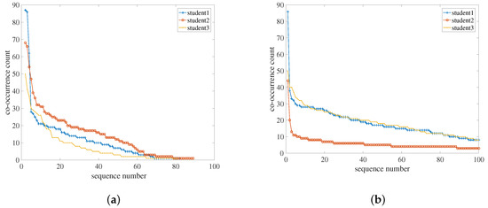
Figure 3.
The scatter plot of co-occurrences between students (1 to 3) and others. The time of co-occurrences here is sorted in descending order for (a) intra-major social ties and (b) inter-major social ties.
For student i, only when confidence is no less than do we consider there is a social tie between student i and student j. Threshold is defined as:
where satisfies:
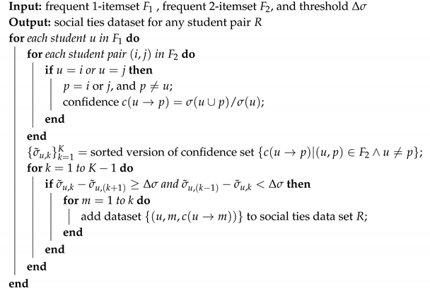
In the above equation, is a parameter; specifically, it is the threshold of difference. From the above definition, we know that student i has social ties with the first k sorted students with the confidence being the strength of the social ties. When mining the social ties of different students, is set to different values so that adapts to different students. In this work, we set the parameter based on a known social sub-network. We did the experiment and adjusted the value of the parameter so that our inferred sub-network fit the known sub-network. Algorithm 5 details the way to obtain social ties data through confidence thresholds.
| Algorithm 5: Obtaining social ties dataset R |
 |
5. Results and Discussion
We collected the student ID card transaction records of 335 students (113 from the electrical engineering (EE) major and 222 from other majors) from the 2012 grade and 327 students from the 2013 grade of CPST, CCNU. Our results were verified by questionnaires or interviews from our investigated students. (For details of the verifications, see Appendix A). Most students often interact with their roommates, friends from the same major, and friends from other majors or grades. The results of the verification showed that our method can extract social ties with better accuracy.
5.1. Mitigation of the Homophily Effects
We compared the social networks extracted using the original model and the networks extracted with our new model. Figure 4 illustrates the results, where nodes are the students and the connection lines are the social ties with their width representing the strength of the connection. In Figure 4a,b, we first investigated the major homophily effect. We labelled the networks from Figure 4a,b by and . There are few connections among the inter-major students without considering the major homophily. In , the proportion of extracted inter-major social ties amongst entire social ties is 0.89% only, while with the hierarchical encounter model shown in , the same proportion grows to 5.45%. We further tested our model by extracting social ties of students from different grades. Social networks inferred with the original model and the new model are illustrated in Figure 4c,d, respectively (labelled with and ). Similar to the previous scenario, the ratio of the inter-grade social ties rises from 0.92% to 4.65% with our new model applied.
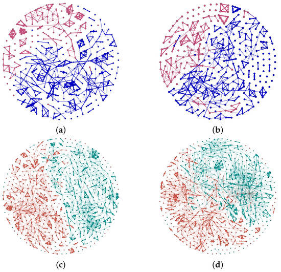
Figure 4.
Social tie revealing alleviation of homophily effects. Here, (a,b) are the social network of 335 students, where red notes represent students from electrical engineering (EE) and blue nodes the others, and (c,d) are the social network of 662 students, where green nodes represent students from grade 2012, and orange nodes students from grade 2013. Networks in (a,c) are extracted with the original model, where the homophily effects are not considered. Networks in (b,d) are extracted by our new model.
To further analyze the inferred networks, we introduced two commonly used measurements [33]. The first one is path length L, which reflects the global characteristic of a network. It represents the average length of every path in a network. The path length is calculated by:
where:
is the average distance from one node to other nodes. From the above equations, we can see that the path length satisfies . When the network is the most centralized and is strongly connected. For convenience, we used the closeness centrality , which is the reciprocal of the average distance of a node , to analyze the network. The closeness centrality is unitless and takes the value from . When , the node is directly connected to any other nodes in the network.
Another measurement is the clustering coefficient, which describes the local characteristic of a network. It shows the degree of convergence of a friend cluster. For a node i with degree (the number of connected adjacent nodes), its clustering coefficient is defined as:
where is the number of lines among the neighbors. The clustering coefficient is also unitless and ranges from 0 to 1. A node with has all its neighbors mutually directly connected.
In Figure 5a,b, we show the closeness centrality and the clustering coefficient of networks and , respectively. Recall here that the network with the prime label represents the network extracted using our method, when, without considering the major homophily, the distribution for the closeness centrality of the social network is more discrete. Compared with , the closeness centrality of increases significantly. We further calculated the path length for the networks and . It turns out that the path length for the network without considering the major homophily is 10.97, while that value is 8.82 when we consider the major homophily. A shorter path length results from an increment of the number of social ties, indicating that more inter-major social ties are found. As illustrated in Figure 5b, since more inter-major social ties are found, the clustering coefficients of network are smaller and are more concentrated when compared to . The average clustering coefficients for a network with or without considering the major homophily are 0.33 and 0.35, respectively. The cluster is slightly more scattered when considering the major homophily, also illustrating that more social ties are extracted.
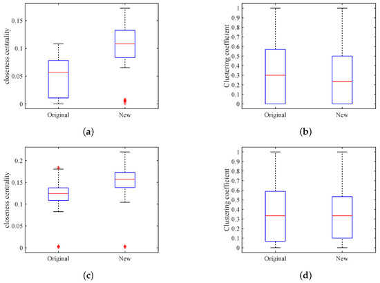
Figure 5.
The boxplot for closeness centrality (a,c) and for clustering coefficient (b,d). Here, the label on the horizontal axis represents networks extracted with the original model or with our new model. Boxplots (a,b) are for networks and , and boxplots (c,d) are for networks and . For each box in the graph, the red ‘+’ represents the extreme outliers.
Similarly, we analyzed networks and by the two measurements. The results are illustrated in Figure 5c,d. In Figure 5c, the central closeness of is larger than 0.1 except for some extreme outliers, which indicates that has more nodes with better observation horizon for information flow. Figure 5d has roughly the same distribution as Figure 5b. With our new model, the path length for the network decreases from 8.96 to 8.20, and the average clustering coefficient drops from 0.39 to 0.37.
Having considered the effect of homophily, our model can mine more genuine inter-major and inter-grade social ties and can infer the social ties of students with better fidelity. We also found that inter-group social ties are far fewer than the intra-group social ties. To facilitate communication between inter-group students and to boost major and grade crossing, the college can organize more activities to help to improve this situation.
5.2. The Effect of the Adaptive Threshold Method
We further investigated the effect of the adaptive threshold determination method. Using the records of the 113 EE students (2012 grade) as examples, we employed the community mining algorithm from Reference [31]. Figure 6a,b illustrates the community network extracted using the traditional fixed threshold method and the adaptive threshold method, respectively. The two networks are labeled with and . In the figures, the nodes represent the students; the sub-networks with various colors and number of nodes are the communities. The isolated nodes scattered across the figures are students without a connection to others. From , we found that there are many connections between communities and there may exist false social ties. By contrast, in , social ties are much more explicit. The number of communities of and are 12 and 14, respectively. In , the maximum number of students in one community is 24, while for , it is 18. The number of communities with 3 to 5 members increases from 6 to 9, indicating that our model rejects some false social ties. For , the modularity is 0.741, and for , the modularity reaches 0.858. This increment further proves the outperformance of our model.
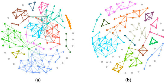
Figure 6.
Social tie inferred from different threshold determination methods with (a) fixed determination method and (b) adaptive determination method. Here, nodes with different colors represent students from a different community.
We analyzed the distribution of the degree value of the two networks and , and the results are illustrated in Figure 7. The degree distribution for the adaptive threshold method tends to concentrate around small values of degree, while that for the fixed threshold method centers around large values of degree. Moreover, the average value of the degree for the adaptive threshold method and that for the fixed threshold method are 2.13 and 2.91, respectively. Usually, a large degree value results from false social ties, while the adaptive threshold method shows higher fidelity.
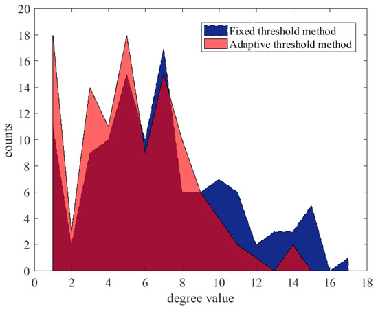
Figure 7.
The distribution for the degree value of the networks mined by the fixed threshold method (dark blue), and by the adaptive threshold method (light red). Here the dark red area represents the overlap between the two areas.
6. Conclusions
To alleviate the homophily effect, we proposed a social network mining method with the student ID card—the hierarchical encounter model based on association analysis. For the social ties of one particular student i, we proposed the following mining procedures. Firstly, calculate the co-occurrences between student i and others using the sliding window method. The traditional association analysis model should then be employed to extract the intra-group students’ social ties. This is followed by the inter-group students’ social ties using quasi-association analysis. The adaptive threshold method is used to sift out weak social ties. Lastly, by combing the social ties of the intra-group students’ social ties and the inter-group students’ social ties, we obtain the complete social ties of student i. We used the data of 662 college students from CPST to verify the effectiveness of our model regarding the homophily and the adaptive thresholds method. Having considered the homophily effect, our new model extracted more inter-group social ties, while with the adaptive threshold method, our model could sift out more false social ties. Results suggested that our model can infer the social ties of students with better fidelity. The method proposed here requires the setting of somewhat arbitrary thresholds (the threshold of difference ) whose selection influences the final result. To determine the influence of the thresholds, a researcher can perform sensitivity analyses to assess how the threshold choices affect results—analyses such as those shown in Figure 6 and Figure 7.
The model we proposed considers issues such as co-occurrence, homophily, and threshold determination. However, several issues remain for future research. Firstly, we did not investigate the setting of the length of the time-window. A length too large risks false social ties, while a length too small may lead to underestimation of the number of social ties [34,35,36,37]. We only considered one characteristic, co-occurrence; it is, however, possible to increase the number of the characteristics [8,38,39], taking into account characteristics such as the number of locations, location entropy, and time entropy. One major limitation of the data comes from the fact that the ID card is exclusive to the food courts and the supermarkets in the university. As more and more students tend to have their meals or shop outside the university, especially through the more and more popular on-line orders, the width and amount of the data will shrink as time goes by. Data from other irreplaceable and commonly visited locations, such as the libraries and the classrooms, can be used to compensate for such an effect.
The applications of our research are manifold. Universities can use our method in a dynamic way. They can infer student social networks every certain period so that the networks are up to date. With the knowledge of students’ social networks, universities can take proactive actions to alleviate possible mental health problems of students and prevent possible damages from students. If contact with a student is lost, universities can contact the friends of this student in the first place. Although there are issues remaining for further study, ID card data may prove a useful tool for mapping social networks based on geographic and temporal proximity when GPS data are unavailable. Because most college campuses have student ID cards, the approach seems particularly useful for monitoring social ties in higher education, particularly in settings where ID cards are frequently used for a variety of activities, such as dining, shopping, rentals, online access, admission to campus activities, and/or library books. We admit that the applicability of our approach might vary across different countries, since for some countries, informed consent of students is hard to get. Nevertheless, our approach can be directly adopted by other Chinese Universities where data collection is relatively easy in the ethical sense due to the special reason we stated in Section 2. Other organizations such as high schools and companies can also adopt our method to monitor the mental status of their students or employees in a similar fashion.
Author Contributions
All authors were involved in the discussion of the methodology. Conceptualization, J.-Y.X., T.L. and S.-Y.L.; Software, J.-Y.X.; Validation, J.-Y.X.; Writing—original draft preparation, J.-Y.X.; Writing—review and editing, T.L., M.L.D. and S.-Y.L.; Visualization, J.-Y.X.; Funding acquisition, L.-T.Y. and S.-Y.L.
Funding
This research was funded by Self-determined research funds of CCNU from the colleges’ basic research and operation of MOE OF FUNDER grant number CCNU17QN0011 and CCNU16JYKX19.
Acknowledgments
Jing-Ya Xu thanks Ming-Jian He for the fruitful discussion.
Conflicts of Interest
The authors declare no conflict of interest.
Appendix A
Appendix A.1. Data Verification
In this work, we used the check-in data of 662 students at food courts or supermarkets from September 2014 to June 2015. The distribution of the students in terms of grade, major, and gender is tabulated in Table A1. The total numbers of the check-in data of students from 2012 grade and 2013 grade are 203,247 and 194,161, respectively.

Table A1.
Distribution of the 662 students in terms of major, gender, and grade. Note: EE denotes the major of electrical engineering, which is further divided into TE (telecommunications engineering), EIE (electronic information Engineering) and EIST (electronic information science and technology). Other majors include PHYN (physics (normal)), PM (physical mathematics) and PHYK (physics (key)).
| Major | Grade 2012 | Grade 2013 | |||||
|---|---|---|---|---|---|---|---|
| Male | Female | Total | Male | Female | Total | ||
| EE | TE | 28 | 36 | 64 | 34 | 23 | 57 |
| EIE | 19 | 18 | 37 | 24 | 7 | 31 | |
| EIST | 9 | 3 | 12 | 12 | 9 | 21 | |
| Others | PHYN | 78 | 75 | 153 | 63 | 80 | 143 |
| PM | 5 | 8 | 13 | 13 | 8 | 21 | |
| PHYK | 30 | 26 | 56 | 30 | 24 | 54 | |
| Total | 169 | 166 | 335 | 176 | 151 | 327 | |
We verified our method with questionnaires and interviews. We designed 64 questionnaires in the electronic form and received 28 valid questionnaires. We also carried out 13 interviews with 2012 grade and 2013 grade students who are now colleagues of the first author of this paper. We mainly used the interview as a supplement for the questionnaires, since such a way of verification consumes much more time than the questionnaire. The questionnaires and the interviews have questions in the same format, but questions for different students might vary. An example of the questionnaire and the interview can be found in Appendix A.2.
The results of the questionnaires and interviews coincide with our inferred social network, proving the validity of our method to some extent. Due to time constrain our insufficient samples of questionnaires cannot prove our method in the general sense. In our future work, we will expand the variety and width of our investigation. We will investigate more students covering a wider range of major, and grade.
Appendix A.2. Sample Questions for Questionnaires and Interviews
A: Bob (2012xxxxxx)
B: Charlie (2012xxxxxx)
C: David (2012xxxxxx)
(1) In the above list, who do you know? ( )
(2) If you know all, who did you usually have a meal together with between Sep 2014 to Jun 2015? ( )
(3) Please list your friends in our college who are not in the list (name, grade).
References
- Hokanson, J.E.; Rubert, M.P.; Welker, R.A.; Hollander, G.R.; Hedeen, C. Interpersonal concomitants and antecedents of depression among college students. J. Abnormal Psychol. 1989, 98, 209. [Google Scholar] [CrossRef]
- Segrin, C.; Flora, J. Poor social skills are a vulnerability factor in the development of psychosocial problems. Hum. Commun. Res. 2000, 26, 489–514. [Google Scholar] [CrossRef]
- Thomas, S.L. Ties That Bind: A Social Network Approach to Understanding Student Integration and Persistence. J. High Educ. 2000, 71, 591–615. [Google Scholar] [CrossRef]
- Brissette, I.; Scheier, M.F.; Carver, C.S. The role of optimism in social network development, coping, and psychological adjustment during a life transition. J. Personal. Soc. Psychol. 2002, 82, 102–111. [Google Scholar] [CrossRef]
- Ellison, N.B.; Steinfield, C.; Lampe, C. The Benefits of Facebook “Friends:” Social Capital and College Students’ Use of Online Social Network Sites. J. Comput.-Mediat. Commun. 2007, 12, 1143–1168. [Google Scholar] [CrossRef]
- Li, Q.; Zheng, Y.; Xie, X.; Chen, Y.; Liu, W.; Ma, W.Y. Mining user similarity based on location history. In Proceedings of the 16th ACM SIGSPATIAL International Conference On Advances in Geographic Information Systems, Irvine, CA, USA, 5–7 November 2008; p. 34. [Google Scholar]
- Chang, J.; Sun, E. Location 3: How users share and respond to location-based data on social networking sites. In Proceedings of the Fifth International AAAI Conference on Weblogs and Social Media, Barcelona, Spain, 17–21 July 2011; pp. 74–80. [Google Scholar]
- Pham, H.; Shahabi, C.; Liu, Y. EBM: An entropy-based model to infer social strength from spatiotemporal data. In Proceedings of the 2013 ACM SIGMOD International Conference on Management of Data, New York, NY, USA, 22–27 June 2013; pp. 265–276. [Google Scholar]
- Cranshaw, J.; Toch, E.; Hong, J.; Kittur, A.; Sadeh, N. Bridging the gap between physical location and online social networks. In Proceedings of the 12th ACM International Conference on Ubiquitous Computing, Copenhagen, Denmark, 26–29 September 2010; pp. 119–128. [Google Scholar]
- Ma, C.; Gui, H.; Liu, H.; Zhu, W.; Xie, L. Inferring social relationship in mobile social networks using tempo-spatial information. In Proceedings of the International Conference on Software Intelligence Technologies and Applications & International Conference on Frontiers of Internet of Things, Hsinchu, Taiwan, 4–6 December 2014. [Google Scholar]
- Xiao, X.; Zheng, Y.; Luo, Q.; Xie, X. Inferring social ties between users with human location history. J. Ambient Intell. Hum. Comput. 2014, 5, 3–19. [Google Scholar] [CrossRef]
- Chung-Huang, Y. On the design of campus-wide multi-purpose smart card systems. In Proceedings of the IEEE 33rd Annual 1999 International Carnahan Conference on Security Technology, Madrid, Spain, 5–7 October 1999; pp. 465–468. [Google Scholar]
- Feng, J.; Feng, L.; Xuan, L. Current situation and development of China Campus Card System. In Proceedings of the 2010 International Conference on Artificial Intelligence and Education (ICAIE), Hangzhou, China, 29–30 October 2010; pp. 469–474. [Google Scholar]
- Fan, S.; Li, P.; Liu, T.; Chen, Y. Population Behavior Analysis of Chinese University Students via Digital Campus Cards. In Proceedings of the 2015 IEEE International Conference on Data Mining Workshop (ICDMW), Atlantic City, NJ, USA, 14–17 November 2015; pp. 72–77. [Google Scholar]
- Jiang, T.; Cao, J.; Su, D.; Yang, X. Analysis and Data Mining of Students’ Consumption Behavior Based on a Campus Card System. In Proceedings of the 2017 International Conference on Smart City and Systems Engineering (ICSCSE), Changsha, China, 11–12 November 2017; pp. 58–60. [Google Scholar]
- Yao, H.; Nie, M.; Su, H.; Xia, H.; Lian, D. Predicting Academic Performance via Semi-supervised Learning with Constructed Campus Social Network. In Proceedings of the International Conference on Database Systems for Advanced Applications; Springer International Publishing: Cham, Switzerland, 2017; pp. 597–609. [Google Scholar]
- Liu, T.; Yang, L.; Liu, S.; Ge, S. Inferring and analysis of social networks using RFID check-in data in China. PLOS ONE 2017, 12, e0178492. [Google Scholar] [CrossRef] [PubMed]
- McPherson, M.; Smith-Lovin, L.; Cook, J.M. Birds of a feather: Homophily in social networks. Annu. Rev. Sociol. 2001, 27, 415–444. [Google Scholar] [CrossRef]
- Kossinets, G.; Watts, D.J. Origins of homophily in an evolving social network. Am. J. Sociol. 2009, 115, 405–450. [Google Scholar] [CrossRef]
- Cohen, J.M. Sources of Peer Group Homogeneity. Sociol. Educ. 1977, 50, 227–241. [Google Scholar] [CrossRef]
- Shrum, W.; Cheek, N.H.; Saundra Mac, D.H. Friendship in School: Gender and Racial Homophily. Sociol. Educ. 1988, 61, 227–239. [Google Scholar] [CrossRef]
- Currarini, S.; Jackson, M.; Pin, P. Identifying Sources of Racial Homophily in High School Friendship. Proc. Natl. Acad. Sci. USA 2018, 107, 4857–4861. [Google Scholar] [CrossRef] [PubMed]
- Currarini, S.; Jackson, M.O.; Pin, P. Identifying the roles of race-based choice and chance in high school friendship network formation. Proc. Natl. Acad. Sci. USA 2010, 107, 4857–4861. [Google Scholar] [CrossRef] [PubMed]
- Kovanen, L.; Kaski, K.; Kertész, J.; Saramäki, J. Temporal motifs reveal homophily, gender-specific patterns, and group talk in call sequences. Proc. Natl. Acad. Sci. USA 2013, 110, 18070–18075. [Google Scholar] [CrossRef] [PubMed]
- Ruan, D.; Zhu, S. Birds of a Feather: A Case Study of Friendship Networks of Mainland Chinese College Students in Hong Kong. Am. Behav. Sci. 2015, 59, 1100–1114. [Google Scholar] [CrossRef]
- Nissi, E.; Muratore, F. Disciplinary homogeneity in university departments following the Gelmini law: An exploratory analysis through social networks. Qual. Quant. 2018. [Google Scholar] [CrossRef]
- Agrawal, R.; Imielinski, T.; Swami, A. Database mining: A performance perspective. IEEE Trans. Knowl. Data Eng. 1993, 5, 914–925. [Google Scholar] [CrossRef]
- Agrawal, R.; Imielinski, T.; Swami, A. Mining association rules between sets of items in large databases. SIGMOD Rec. 1993, 22, 207–216. [Google Scholar] [CrossRef]
- Curme, C.; Tumminello, M.; Mantegna, R.N.; Stanley, H.E.; Kenett, D.Y. Emergence of statistically validated financial intraday lead-lag relationships. Quant. Financ. 2015, 15, 1375–1386. [Google Scholar] [CrossRef]
- Li, M.X.; Palchykov, V.; Jiang, Z.Q.; Kaski, K.; Kertész, J.; Miccichè, S.; Tumminello, M.; Zhou, W.X.; Mantegna, R.N. Statistically validated mobile communication networks: The evolution of motifs in European and Chinese data. New J. Phys. 2014, 16, 083038. [Google Scholar] [CrossRef][Green Version]
- Tang, P.; Turkia, M.P. Parallelizing Frequent Itemset Mining with FP-Trees. In Proceedings of the International Conference on Computers and Their Applications, Cata, Seattle, WA, USA, 23–25 March 2006; pp. 30–35. [Google Scholar]
- Sbora, C. Indicators for Determining Collaborative Security Level in Organizational Environments. Inf. Econ. J. 2014, 18, 131–143. [Google Scholar] [CrossRef]
- Wasserman, S.; Faust, K. Social Network Analysis: Methods and Applications; Cambridge University Press: Cambridge, UK, 1994; Volume 8. [Google Scholar]
- Psorakis, I.; Voelkl, B.; Garroway, C.J.; Radersma, R.; Aplin, L.M.; Crates, R.A.; Culina, A.; Farine, D.R.; Firth, J.A.; Hinde, C.A.; et al. Inferring social structure from temporal data. Behav. Ecol. Sociobiol. 2015, 69, 857–866. [Google Scholar] [CrossRef]
- Krause, J.; Krause, S.; Arlinghaus, R.; Psorakis, I.; Roberts, S.; Rutz, C. Reality mining of animal social systems. Trends Ecol. Evol. 2013, 28, 541–551. [Google Scholar] [CrossRef] [PubMed]
- Shi, J.; Mamoulis, N.; Wu, D.; Cheung, D.W. Density-based place clustering in geo-social networks. In Proceedings of the 2014 ACM SIGMOD International Conference On Management of Data, Snowbird, UT, USA, 22–27 June 2014; pp. 99–110. [Google Scholar]
- Psorakis, I.; Roberts, S.J.; Rezek, I.; Sheldon, B.C. Inferring social network structure in ecological systems from spatio-temporal data streams. J. R. Soc. Interface 2012. [Google Scholar] [CrossRef] [PubMed]
- Luo, H.; Guo, B.; Yu, Z.W.; Wang, Z.; Feng, Y. Friendship Prediction Based on the Fusion of Topology and Geographical Features in LBSN. In Proceedings of the 2013 IEEE 10th International Conference on High Performance Computing and Communications & 2013 IEEE International Conference on Embedded and Ubiquitous Computing, Zhangjiajie, China, 13–15 November 2013; pp. 2224–2230. [Google Scholar]
- Scellato, S.; Noulas, A.; Mascolo, C. Exploiting place features in link prediction on location-based social networks. In Proceedings of the 17th ACM SIGKDD International Conference On Knowledge Discovery and Data Mining, San Diego, California, USA, 21–24 August 2011; pp. 1046–1054. [Google Scholar]
© 2019 by the authors. Licensee MDPI, Basel, Switzerland. This article is an open access article distributed under the terms and conditions of the Creative Commons Attribution (CC BY) license (http://creativecommons.org/licenses/by/4.0/).