A New Flexible Sigmoidal Growth Model

Abstract

Biological growth is driven by numerous functions, such as hormones and mineral nutrients, and is also involved in various ecological processes. Therefore, it is necessary to accurately capture the growth trajectory of various species in ecosystems. A new sigmoidal growth (NSG) model is presented here for describing the growth of animals and plants when the assumption is that the growth rate curve is asymmetric. The NSG model was compared with four classic sigmoidal growth models, including the logistic equation, Richards, Gompertz, and ontogenetic growth models. Results indicated that all models fit well with the empirical growth data of 12 species, except the ontogenetic growth model, which only captures the growth of animals. The estimated maximum asymptotic biomass $w_{max}$ of plants from the ontogenetic growth model was not reliable. The experiment result shows that the NSG model can more precisely estimate the value and time of reaching maximum biomass when growth rate becomes close to zero near the end of growth. The NSG model contains three other parameters besides the value and time of reaching maximum biomass, and thereby, it can be difficult to assign initial values for parameterization using local optimization methods (e.g., using Gauss–Newton or Levenberg–Marquardt methods). We demonstrate the use of a differential evolution algorithm for resolving this issue efficiently. As such, the NSG model can be applied to describing the growth patterns of a variety of species and estimating the value and time of achieving maximum biomass simultaneously.

1. Introduction

The growth of individual biomass is driven by numerous functions and processes, as well as interspecific interactions [1,2,3,4,5]. Normally, the growth rate increases sharply at the initial stage, reaching a peak, and then decreases to zero when the weight or biomass of the organism reaches its maximum [6,7]. As a result, the growth rate curve is often bell-shaped, such as the growth rate of bacteria and insects responding to temperature change [8,9,10,11]. As such, a complete trajectory of biomass growth resembles a sigmoidal curve [12,13]. Many sigmoidal growth models have been proposed to capture the growth trajectory with accuracy, such as the classical logistic equation and models proposed by Gompertz and by Richards [6,14]. The logistic equation describes the symmetric growth, whereas the Gompertz and ontogenetic growth equations depict asymmetric growth with fixed inflection points. In contrast, the inflection point of the Richards equation is flexible and can be used for describing different levels of asymmetry in growth [15]. In addition, Reference also presented a general ontogenetic growth equation based on the 3/4 power law of allometric scaling [16,17].

(i) Logistic equation [18,19]:

$$w=\frac{w_{max}}{1+e^{-k\left(t-t_m\right)}}$$

(1)

where w is the biomass at time t, k the rate of growth, and $t_m$ the inflection point when the growth rate reaches the peak and the biomass reaches the half of its asymptotic maximum value ($w_{max}$).

(ii) Gompertz equation [20,21]:

$$w=w_{max}{e}^{-e^{-k\left(t-t_m\right)}}$$

(2)

where $t_m$ is the time when the growth rate reaches the peak and the biomass reaches $w_{max}/e$.

(iii) Richards equation [22,23]:

$$w=\frac{w_{max}}{{\left[1+v{e}^{-k\left(t-t_m\right)}\right]}^{1/v}}$$

(3)

where v is a model constant and $t_m$ the time when the growth rate reaches the peak and the biomass reaches $w_{max}$, the asymptotic maximum biomass.

(iv) Ontogenetic growth equation:

$$w=w_{\max }{\left\{1-\left[1-{\left(w_0/w_{\max }\right)}^{1/4}\right]\cdot \exp \left[-at/\left(4w_{\max }^{1/4}\right)\right]\right\}}^4$$

(4)

where a is a constant and $w_0$ the initial biomass at t = 0.

Both the logistic and the Gompertz equations have three parameters, including $t_m$ for maximum growth rate, the model constant $k$, and the asymptotic biomass $w_{max}$. The Richards equation becomes the logistic and Gompertz equations, respectively, when $v=1$ and $v=0$ [24,25]. The ontogenetic growth equation also has three parameters, with the main ones being $w_0$ and $w_{max}$.

Although all these models can predict the asymptotic $w_{max}$, a conceptual maximum biomass, all suffer from inaccuracy of their predictions. As variation of biological growth is ubiquitous among individuals and populations [26], random-effect models have been used to improve the accuracy of predictions in recent studies [27,28,29]. As the actual value of $w_{max}$ is a crucial index to assess yield and productivity of crops and livestock, it is therefore necessary to propose a new sigmoidal growth (NSG) model to address the problem of inaccurate predictions.

There are many statistical software packages currently available for estimating parameters in nonlinear models [30,31], among which nls and optim are two functions in R for fitting nonlinear models [32]. The main algorithms implemented in these two functions belong to local optimization, such as the Gauss–Newton and Nelder–Mead algorithms. Local optimization algorithms are typically sensitive to initial values assigned to model parameters. Failed convergence often occurs due to wrong selection of initial values. Local optimal solutions could be misidentified as the parameter estimates. No reliable methods exist for the choice of initial values [7].

To develop effective methods for resolving the conundrum of assigning appropriate initial values when fitting nonlinear growth models, we need to go beyond local optimization. The differential evolution (DE) algorithm is a heuristic global optimization algorithm, which is less sensitive to assigned initial values [33,34]. There are four main steps for the DE algorithm: initialization, mutation, crossover, and selection, and the algorithm is also capable of dealing with nondifferentiable problems [35]. Comparisons show that the DE algorithm performs better than other global optimization methods, such as the genetic algorithm and simulated annealing [35,36]. As such, the DE algorithm has been widely applied in other research fields [37,38]. However, the use of the DE algorithm for the parameterization of nonlinear growth models is yet to be assessed.

Here, we aim to propose a new general sigmoidal growth model with a flexible inflection point that can estimate both the value of the maximum biomass and the time to reach it. In addition, we also attempt to develop a reliable method for fitting the nonlinear growth models, including the new sigmoidal growth model, using the DE algorithm to simultaneously solve the issue of hyper initial-value sensitivity when applying local optimization algorithms.

2. Materials and Methods

2.1. Mathematical Model

Temperature plays a significant role in controlling the developmental rate of biological growth of both plants and animals. There exist lower and upper developmental thresholds for many ectotherms [11]. For example, arthropods will not develop when temperature is below the lower developmental threshold. Developmental rate increases sharply when temperature is higher than the lower threshold and rapidly decreases to zero when temperature reaches the upper threshold. The authors of [10] proposed a model to describe how developmental rate (R) in arthropods responds to the changes in ambient temperature (T):

$$R\left(T\right)=\{\begin{array}{ll}0\hfill & for T\le T_0\hfill \\ aT\left(T-T_0\right){\left(T_L-T\right)}^{1/b}\hfill & for T_0\le T\le T_L\hfill \\ 0\hfill & for T\ge T_L\hfill \end{array}$$

(5)

where a and b are constants controlling the slope of a curve and $T_0$ and $T_L$ represent the lower and upper developmental thresholds, respectively. Similarly, the growth rate also increases sharply in the initial temporal stage and then decreases to zero along with time, resembling to the response of growth to temperature. The growth of plants and poikilotherms seriously depends on environmental factors, especially temperature. The effect of temperature on the growth rate exhibits a typically left-skewed curve [39]. This curve is similar to that generated by a beta function [40]. In general, the distribution of energy in a limited space and time exhibits such a distributional characteristic [41]. For instance, the distribution of daily or monthly precipitation in an area can be well described by the beta function [42]. In the growth of plants, the growth rate curve (versus time) reflects the difference of the abilities of plants at their different growth stages transferring abiotic energy to biotic energy. In the whole height growth process, daily change in biomass also follows a beta growth pattern [43]. As such, it is feasible to substitute the temperature with the temporal variable in Equation (5) in light of the similarity of growth patterns. Here, after replacing the temperature with the analogy of time, we suggest to use the accumulative form of developmental rate, by integrating Equation (5) as the new sigmoidal growth equation for $m<t<n$:

$$w=w_{max}-\frac{ab{\left(n-t\right)}^{1+\frac{1}{b}}\left\{t\left(t-m\right)+b\left\{\left[t\left(2n+3t\right)-m\left(n+4t\right)\right]+b^2\left[-3m\left(n+t\right)+2\left(n^2+nt+t^2\right)\right]\right\}\right\}}{\left(1+b\right)\left(1+2b\right)\left(1+3b\right)}$$

(6)

where a, b, m, n, and $w_{max}$ are model parameters. When $t\le m, t=m;t\ge n,t=n$.

2.2. Parameter Estimation

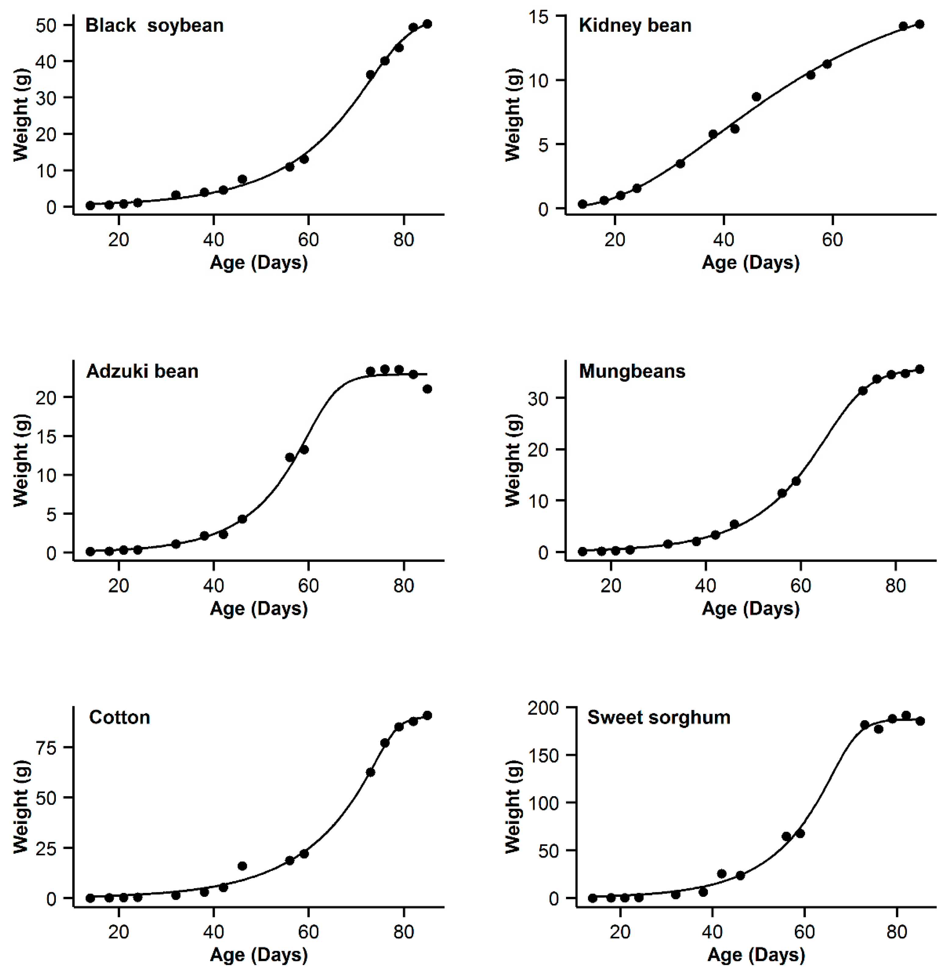
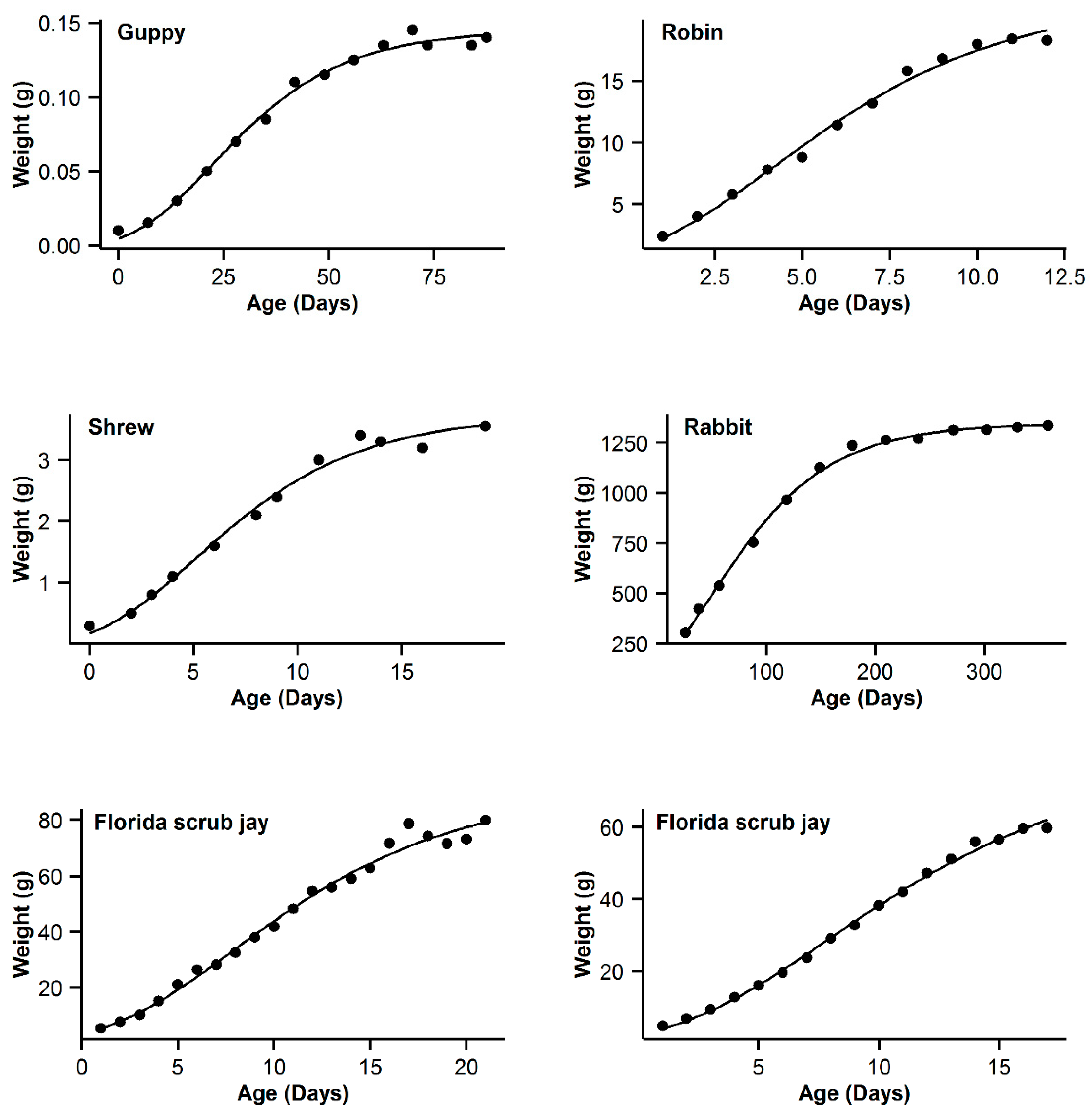
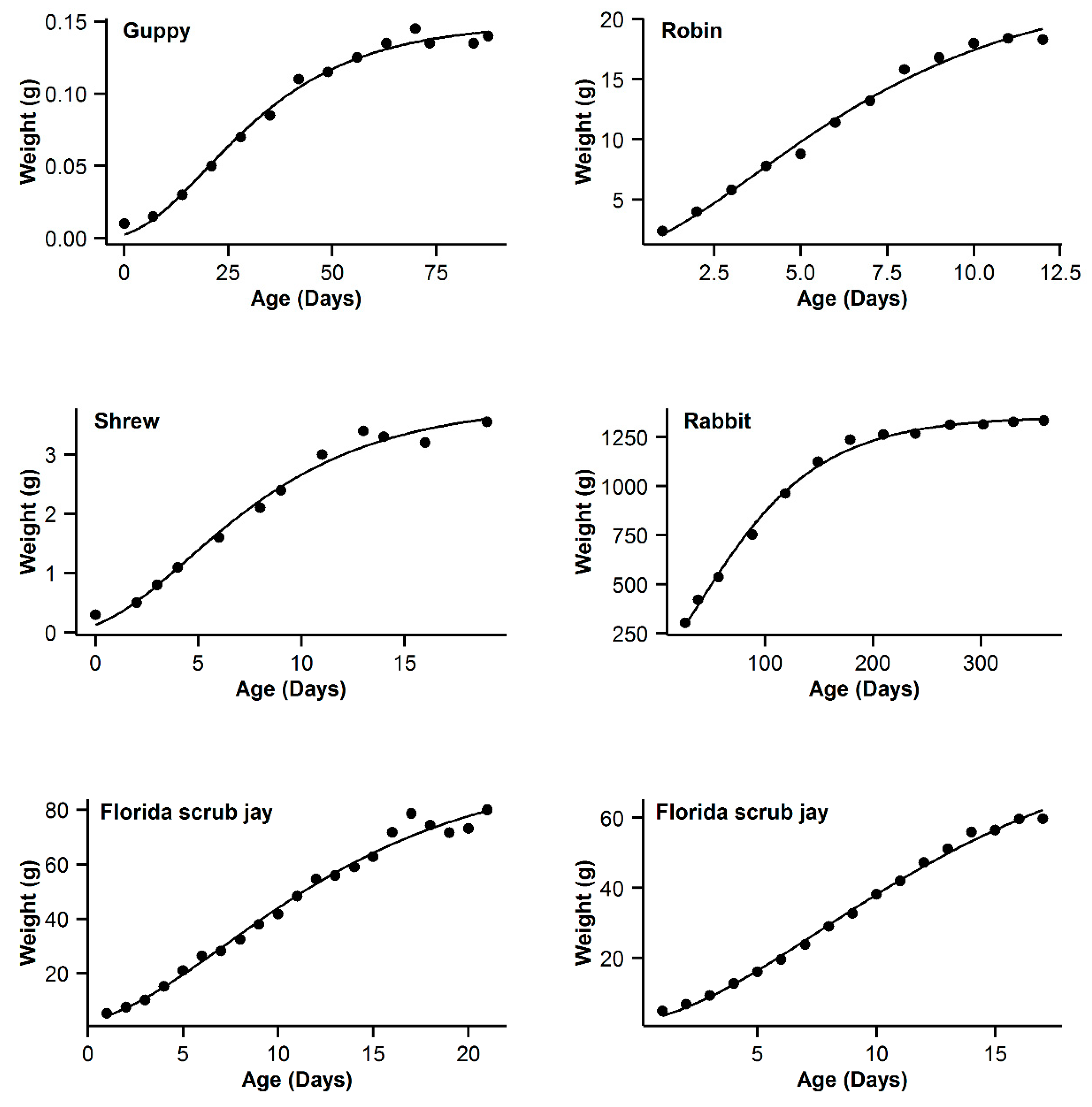
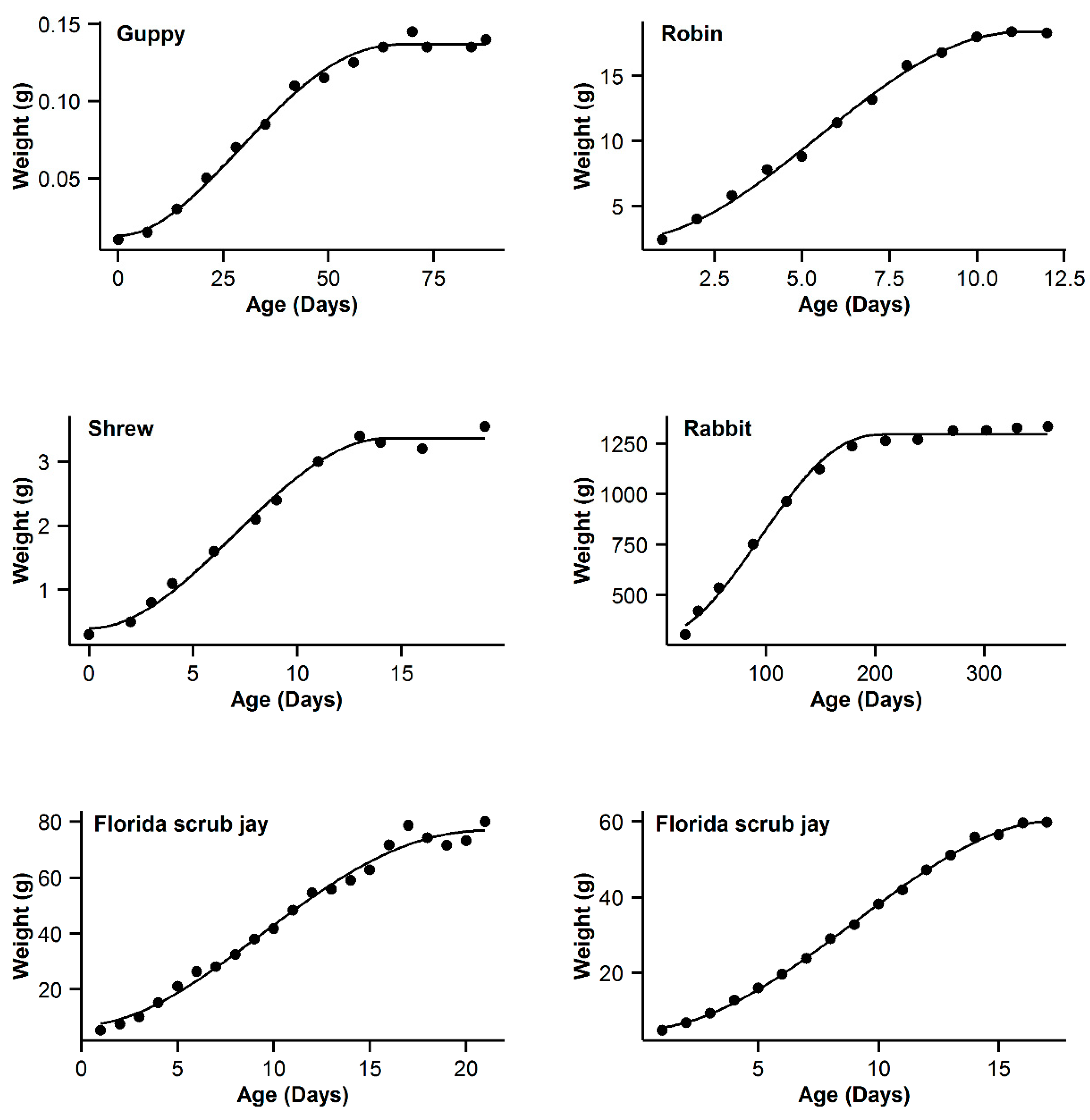
We estimated all five models of biomass growth using the DE and the Nelder–Mead algorithms to minimize the sum of squared errors between observed and predicted values, implemented in the R package DEoptim [44] and the optim function of R [32], respectively. We used the coefficient of determination, $R^2$, for evaluating the goodness of fit and Akaike’s information criterion for model comparison (AIC; [45,46]). The values of $R^2$ and AIC are calculated according to the following formula:

$$R^2=SSR/SST$$

(7)

$$AIC=nln\left(\frac{SSR}{n}\right)+2k$$

(8)

with $SSR={{\displaystyle \sum }}_{i=1}^n{\left(y_i-{\widehat{y}}_i\right)}^2$ and $SST={{\displaystyle \sum }}_{i=1}^n{\left(y_i-\overline{y_i}\right)}^2$, where n represents the sample size, y_i the ith observation of biomass, $\hat{y}$_i the predicted biomass, n the sample size, and k the number of parameters in the growth model.

We tested these models using growth datasets of 12 species, including datasets of six plant species: black soybean, kidney bean, adzuki bean, mung bean, cotton, and sweet sorghum [47] and six animal species: datasets of guppy, robin, shrew, and rabbit [15] and datasets of Florida scrub jay [48] and Western scrub jay [49].

3. Results

The five growth models can be divided into three groups depending on their number of parameters: the five-parameter NSG model in Equation (5), the four-parameter Richards model in Equation (3), and three three-parameter models (logistic in Equation (1), Gompertz in Equation (2), and ontogenetic in Equation (4)). When fitting the parameters for the real datasets, it took about 12 seconds and 500 iterations for the differential evolution (DE) algorithm to parameterize the NSG model of Equation (5), compared to only 5 s needed for fitting the other models. The DE algorithm was robust against different initial parameter values (

Table 1. Lower and upper bounds of parameters of each model optimized by differential evolution method. NSG and OGM represent the new growth model and the ontogenetic growth model, respectively.

Model	Parameter	Lower Bound	Upper Bound
	a	1.00 × 10−9	1.00 × 10−3
	b	0	5
NSG	$w_{max}$	0	300
	m	−200	200
	n	0	500
	$w_{max}$	0	500
Richards	k	0	1
	$t_m$	0	500
	v	0	1
	$w_{max}$	0	500
Logistic	k	0	1
	$t_m$	0	500
	$w_{max}$	0	500
Gompertz	k	0	1
	$t_m$	0	500
	$w_{max}$	0	500
OGM	$w_0$	0	1
	a	0	1

), with preliminary requirements on parameter bounds satisfied (specifically, biomass ranges from 0.1 to 1000 and time ranges from 0.1 to 500). All datasets met the requirements, except those for guppy and rabbit, and we therefore multiplied the guppy biomass by 100 and the time and biomass of rabbit by 0.1 and 0.01, respectively. The DE algorithm also worked well for the logistic and Gompertz models $(R^2>0.98)$ after setting the lower and upper bounds of initial values to between 0 and 500. After setting the parameters estimated from the DE algorithm as initial values, the Nelder–Mead method also performed well with no convergence failures occurring. As such, the use of the DE algorithm can efficiently resolve the hypersensitivity to initial values in the local optimization algorithm and estimate parameters in highly nonlinear models with accuracy.

For the six plant species, the NSG and three classic sigmoidal models performed well, with $R^2$ values of approximately 0.99 (

Table 2. Akaike’s information criterion (AIC) and R² values of the five growth models for the datasets of plants and animals. NSG and OGM represent the new sigmoidal growth model and the ontogenetic growth model, respectively.

Code	Models Name	NSG			Logistic			Gompertz			Richards			OGM
	Species	R2	AIC	ΔAIC	R2	AIC	ΔAIC	R2	AIC	ΔAIC	R2	AIC	ΔAIC	R2	AIC	ΔAIC
1	Black soybean	0.995	18.77	15.63	0.996	11.14	8	0.993	20.91	17.77	0.998	3.14	0	0.985	31.04	27.9
2	Kidney bean	0.993	−11.08	10.48	0.991	−11.89	9.67	0.996	−21.56	0	0.996	−20.24	1.32	0.995	−17.94	3.62
3	Adzuki bean	0.995	−1.55	0.3	0.992	1.65	3.5	0.987	9.18	11.03	0.995	−1.85	0	0.953	28.95	30.8
4	Mung bean	0.998	−11.75	11.5	0.998	−4.21	19.04	0.993	12.88	36.13	0.999	−23.25	0	0.978	29.21	52.46
5	Cotton	0.994	40.29	9.64	0.993	37.98	7.33	0.99	44.77	14.12	0.996	30.65	0	0.966	62.58	31.93
6	Sweet sorghum	0.996	58.22	3.31	0.993	63.47	8.56	0.986	73.23	18.32	0.996	54.91	0	0.949	93.06	38.15
7	Guppy	0.993	−16.84	5.89	0.994	−22.73	0	0.993	−19.8	2.93	0.995	−21.54	1.19	0.991	−16.28	6.45
8	Robin	0.997	−16.61	0.47	0.995	−17.08	0	0.992	−11.29	5.79	0.99	−5.85	5.44	0.991	−9.26	7.82
9	Shrew	0.992	−44.98	3.76	0.992	−48.74	0	0.989	−44.68	4.06	0.992	−46.96	1.78	0.987	−42.53	6.21
10	Rabbit	0.994	−22.52	22.03	0.998	−44.55	0	0.997	−36.5	8.05	0.998	−42.57	1.98	0.996	−32.82	11.73
11	Florida scrub jay	0.989	50.13	3.51	0.988	47.39	0.77	0.989	46.62	0	0.989	48.21	1.59	0.988	47.63	1.01
12	Western scrub jay	0.999	−10.43	0	0.999	−8.05	2.38	0.997	5.09	15.52	0.999	−5.92	4.51	0.996	11.03	21.46

). The ontogenetic growth equation can also fit the data ($R^2>0.94)$, but worse than for the other four growth models (Table 2). All five models fit well with the data from the six animal species, with $R^2$ values of approximately 0.99 (Table 2). The goodness-of-fit of the NSG model for four out of the six animal species was the highest when compared to the other models (Table 2). According to the AIC, the Richards and the logistic models performed the best in most cases for the plant species and animal species, followed by the NSG and the Richards models (Table 2).

In addition, the NSG and Richards growth models overestimated the initial biomass of crop species (Figure 1 and Figure 2, Supporting Information). Meanwhile, the Gompertz and ontogenetic models underestimated the initial animal biomass (Figure 3 and Figure 4), while the NSG, logistic, and Richards models overestimated the initial biomass of animal species (Figure 5, Figure 6 and Figure 2). Compared to the NSG model, the other four models predicted an asymptotic biomass higher than the maximum weight of crop species in the datasets (

Table 3. Estimated parameter values of the five growth models for the datasets of plants and animals. NSG and OGM represent the new growth model and the ontogenetic growth model, respectively.

Species	NSG					Richards				Logistic			Gompertz			OGM
	a	b	${\mathit{w}}_{\mathit{m}\mathit{a}\mathit{x}}$	m	n	${\mathit{w}}_{\mathit{m}\mathit{a}\mathit{x}}$	k	${\mathit{t}}_{\mathit{m}}$	v	${\mathit{w}}_{\mathit{m}\mathit{a}\mathit{x}}$	k	${\mathit{t}}_{\mathit{m}}$	${\mathit{w}}_{\mathit{m}\mathit{a}\mathit{x}}$	k	${\mathit{t}}_{\mathit{m}}$	${\mathit{w}}_{\mathit{m}\mathit{a}\mathit{x}}$	${\mathit{w}}_0$	a
Black soybean	3.24 × 10−4	4.79	50.76	30.36	83.23	52.77	0.25	72.76	3.58	67.31	0.09	72.14	147.76	0.03	86.00	510.94	1.00 × 10−25	0.19
Kidney bean	6.77 × 10−6	1.23	14.20	−26.41	72.41	17.75	0.04	39.00	−0.20	14.80	0.10	44.60	16.79	0.05	40.33	20.07	1.03 × 10−24	0.29
Adzuki bean	7.64 × 10−5	1.49	22.91	29.55	73.55	22.94	0.35	59.72	3.67	23.59	0.15	55.99	24.93	0.09	52.03	67.98	2.43 × 10−24	0.21
Mung bean	2.44 × 10−4	3.96	35.10	26.54	77.34	35.28	0.28	65.34	3.32	38.43	0.13	62.40	46.57	0.06	60.23	305.78	5.72 × 10−24	0.18
Cotton	8.40 × 10−4	8.91	88.95	29.86	80.31	90.05	0.54	74.05	7.52	111.70	0.11	69.94	180.64	0.04	73.99	521.88	1.00 × 10−25	0.24
Sweet sorghum	2.33 × 10−3	11.02	185.78	27.48	74.06	186.95	0.43	65.45	4.71	201.58	0.14	61.72	236.38	0.07	59.17	524.10	1.05 × 10−24	0.35
Guppy	1.37 × 10−7	0.66	13.68	−246.67	68.91	14.15	0.08	26.84	0.64	14.02	0.09	28.80	14.56	0.06	22.02	14.82	0.26	0.38
Robin	7.90 × 10−4	0.86	18.38	−59.23	11.30	24.11	0.19	3.88	−0.27	19.75	0.44	5.20	21.79	0.26	4.17	22.87	0.89	1.87
Shrew	8.18 × 10−5	0.82	3.37	−40.70	14.47	3.50	0.41	6.98	1.37	3.54	0.36	6.60	3.74	0.22	5.04	3.85	0.13	1.05
Rabbit	5.17 × 10−5	0.61	12.95	−20.15	21.01	13.27	0.23	7.44	0.96	13.26	0.23	7.51	13.47	0.17	5.07	13.55	1.06	1.15
Florida scrub jay	1.11 × 10−4	0.72	76.97	−141.30	21.55	86.55	0.19	8.57	0.32	81.51	0.26	9.57	90.91	0.15	7.91	96.25	2.30	1.54
Western scrub jay	3.18 × 10−4	1.07	59.99	−226.33	17.12	67.06	0.28	8.76	0.83	65.99	0.30	8.91	78.65	0.16	7.93	87.04	1.76	1.47

where a, b, m, n are model parameters, and $w_{max}$. Maximum biomass, k the rate of growth, and $t_m$ the inflection point when the growth rate reaches the peak and the biomass reaches the half of its asymptotic maximum value ($w_{max}$), v is a model constant, $w_0$ the initial biomass at t = 0.

). Similarly, the estimates of $w_{max}$ for the animal species from the logistic, Gompertz, Richards and ontogenetic models were higher than those from the NSG model (Table 3 and

Table 4. The ratio of estimated to observed values of maximum biomass. NSG and OGM represent the new growth model and the ontogenetic growth model, respectively.

Species	Observed (g)	NSG	Richards	Logistic	Gompertz	OGM
Black soybean	50.20	1.01	1.05	1.34	2.94	10.18
Kidney bean	14.35	0.99	1.24	1.03	1.17	1.40
Adzuki bean	23.60	0.97	0.97	1.00	1.06	2.88
Mung bean	35.60	0.99	0.99	1.08	1.31	8.59
Cotton	90.80	0.98	0.99	1.23	1.99	5.75
Sweet sorghum	191.50	0.97	0.98	1.05	1.23	2.74
Guppy	0.15	0.94	0.98	0.97	1.00	1.02
Robin	18.40	1.00	1.31	1.07	1.18	1.24
Shrew	3.55	0.95	0.99	1.00	1.05	1.08
Rabbit	1335.00	0.97	0.99	0.99	1.01	1.01
Florida scrub jay	80.00	0.96	1.08	1.02	1.14	1.20
Western scrub jay	59.75	1.00	1.12	1.10	1.32	1.46

). Estimates of $w_{max}$ of crop species from the NSG, Richards, and logistic models were relatively similar to each other (Table 3 and Table 4). Estimates of $w_{max}$ of crop species from the Gompertz and ontogenetic models were often much higher than those of the other three models (Table 3 and Table 4). For example, the estimates of $w_{max}$ for the black soybean, cotton, and sweet sorghum when using the Gompertz and ontogenetic models were more than those of the estimates from the other three models (Table 3). Estimates of $t_m$ of crop species from the logistic, Gompertz, and Richards models were similar to each other (Table 3). Among the five growth models, only the NSG model was able to predict the time of reaching $w_{max}$ when the crop growth ceases (Figure 1 and Table 3). In contrast, for the crop species, the ontogenetic model could predict neither $t_m$ for maximum growth rate nor the time of reaching maximum biomass. In summary, the results suggested that only the NSG model can accurately predict the timing and value of $w_{max}$ for all the 12 datasets, including crop species (Figure 7, Figure 8 and Figure 9) and animal species (Figure 5 and Table 3).

4. Discussion

The results showed that the NSG and Richards models fit the data well ($R^2>0.98)$ and predicted similar estimates of $w_{max}$ and initial biomass (Table 2). Both the Gompertz and ontogenetic models underestimated the initial weight of animal species (Figure 4 and Figure 6), while the logistic equation overestimated the initial weight (Figure 6). The estimates of $w_{max}$ from the Gompertz and ontogenetic models for plants were much higher than those from the other models (Table 3 and Table 4). Different performance among models in estimating $w_{max}$ and the initial weight can be explained by the forms of these growth equations. The logistic, Richards, and Gompertz models assume w = 0 when t = 0; in most cases, this assumption is reasonable, such as for plants germinated from seeds. However, it is rather unsuitable for describing the growth of animals, especially mammals.

It is critical for a growth model to have a flexible inflection point due to the existence of both symmetric and asymmetric growth [7]. The logistical equation is symmetric and has an the inflection point at $w_{max}/ 2$; the Gompertz and ontogenetic models are asymmetric and have their inflection points, respectively, at $w_{max}/e$ and $8w_{max}/27$ [50]. In contrast, the inflection point of the Richards equation is flexible, often used for capturing different levels of asymmetry in growth. The NSG model is also asymmetric and has a flexible inflection point. According to the flexibility of the inflection point, we can classify these models into three groups: group I (symmetric with a fixed inflection point): the logistical equation; group II (asymmetric with a fixed inflection point): the Gompertz and ontogenetic growth equations; and group III (asymmetric with a flexible inflection point): the Richards and the NSG models. Evidently, the estimates of $w_{max}$ and initial weights were similar from models of the same group. Environmental complexity and biotic interactions could further deviate the growth curve from a perfect sigmoidal curve. As such, the estimates of $w_{max}$ from the logistic, Richards, Gompertz, and ontogenetic growth models were higher than the observed values of $w_{max}$. The NSG model assumes a zero rate when growth ceases, making its estimates of $w_{max}$ closer to the observed values.

The ontogenetic model fitted the growth of animals much better than that of plants (Figure 4 and Figure 8 and Table 2). The estimates of $w_{max}$ for plants from the ontogenetic growth model were not reliable (Table 3), suggesting it not a general model for all the species [47]. The ontogenetic growth model is based on the 3/4 power law [17,51], and the 3/4 exponent is an empirical index based mainly on the interspecific relationship between basal metabolic rate and biomass of animals [52,53]. Although some have argued the universality of the 3/4 power law [54] and whether it should also be suitable for describing plants [55], evidence does exist of the wide discrepancies in exponents among different taxa [56,57,58,59], even for individuals within the same species [26]. Therefore, the allometric power law might not be universal and could not be applied for all species.

Although there are many sigmoidal growth models such as those listed here that have been widely used in describing various growth trajectories, new models are still being proposed for improved accuracy in predictions of the final maximum biomass [60,61]. All the models consider $w_{max}$ as the upper asymptote and cannot estimate the actual final biomass when the growth ceases. The NSG model proposed here can not only predict the final biomass $w_{max}$, but also the timing of reaching $w_{max}$ when the growth ceases. The NSG model performed similarly to the logistic and Richards equations and better than the Gompertz and ontogenetic growth models due to having a flexible inflection point. Therefore, this new sigmoidal growth model can be applied to describing the growth trajectories of many species.

The main drawback of the NSG model is the number of parameters. Reasonably adding the number of model parameters surely can improve the fitting flexibility of the model, and consequently enhance the goodness-of-fit of data fitting. However, too many parameters will increase the model’s complexity and require a large sample size in order to accurately estimate those parameters. Thus, in the model’s valuation, the trade-off between the goodness of fit and the complexity of model structure is usually considered [62]. The AIC as an indicator in model comparison exactly played such a role [63]. In the current study, our new sigmoid function has the lowest AIC, which indicates the model validity and superiority to the other models. In this case, the number of parameters actually has been weighed in the calculation of the AIC value. It is difficult to set the correct initial values of parameters, compared to other models with lower numbers of parameters, when using local optimization algorithms, such as the Gauss–Newton and Levenberg–Marquardt algorithms. Fortunately, our results indicated that the DE algorithm of global optimization can predict estimates of model parameters with accuracy and efficiently resolve the issue of initial-value hypersensitivity in algorithms of local optimization with only a slightly longer but bearable running time, consistent with the results from other studies on comparing evolutionary algorithms [35]. The compensation of running time for robust estimates against changes in initial parameter values suggests the use of DE algorithm to be a recommendable choice. For this reason, we recommend the use of the DE algorithm in global optimization for estimating parameters of the NSG model. As demonstrated, the DE algorithms can successfully estimate the parameters of the NSG model for all tested species under the same initial values. In conclusion, the proposed model of asymmetric growth, with its flexible inflection point, can be applied to a variety of taxa for capturing their growth trajectories, especially when using the differential evolution algorithm of global maximization.

References

1. Vermeij, M. Early life-history dynamics of Caribbean coral species on artificial substratum: The importance of competition, growth and variation in life-history strategy. Coral Reefs 2006, 25, 59–71. [Google Scholar] [CrossRef]
2. Zhao, D.; Borders, B.; Wilson, M. Individual-tree diameter growth and mortality models for bottomland mixed-species hardwood stands in the lower Mississippi alluvial valley. For. Ecol. Manag. 2004, 199, 307–322. [Google Scholar] [CrossRef]
3. Lhotka, J.M.; Loewenstein, E.F. An individual-tree diameter growth model for managed uneven-aged oak-shortleaf pine stands in the ozark Highlands of Missouri, USA. For. Ecol. Manag. 2011, 261, 770–778. [Google Scholar] [CrossRef]
4. Holland, E.P.; Pech, R.P.; Ruscoe, W.A.; Parkes, J.P.; Nugent, G.; Duncan, R.P. Thresholds in plant–herbivore interactions: Predicting plant mortality due to herbivore browse damage. Oecologia 2013, 172, 751–766. [Google Scholar] [CrossRef]
5. Scogings, P.F.; Hjältén, J.; Skarpe, C.; Hattas, D.; Zobolo, A.; Dziba, L.; Rooke, T. Nutrient and secondary metabolite concentrations in a savanna are independently affected by large herbivores and shoot growth rate. Plant Ecol. 2014, 215, 73–82. [Google Scholar] [CrossRef]
6. Zeide, B. Analysis of growth equations. For. Sci. 1993, 39, 594–616. [Google Scholar] [CrossRef]
7. Archontoulis, S.V.; Miguez, F.E. Nonlinear regression models and applications in agricultural research. Agron. J. 2015, 107, 786–798. [Google Scholar] [CrossRef]
8. Ratkowsky, D.; Olley, J.; McMeekin, T.; Ball, A. Relationship between temperature and growth rate of bacterial cultures. J. Bacteriol. 1982, 149, 1–5. [Google Scholar]
9. Ratkowsky, D.; Lowry, R.; McMeekin, T.; Stokes, A.; Chandler, R. Model for bacterial culture growth rate throughout the entire biokinetic temperature range. J. Bacteriol. 1983, 154, 1222–1226. [Google Scholar]
10. Briere, J.-F.; Pracros, P.; Le Roux, A.-Y.; Pierre, J.-S. A novel rate model of temperature-dependent development for arthropods. Environ. Entomol. 1999, 28, 22–29. [Google Scholar] [CrossRef]
11. Lactin, D.J.; Holliday, N.; Johnson, D.; Craigen, R. Improved rate model of temperature-dependent development by arthropods. Environ. Entomol 1995, 24, 68–75. [Google Scholar] [CrossRef]
12. Miguez, F.E.; Villamil, M.B.; Long, S.P.; Bollero, G.A. Meta-analysis of the effects of management factors on miscanthus× giganteus growth and biomass production. Agric. For. Meteorol. 2008, 148, 1280–1292. [Google Scholar] [CrossRef]
13. Sebens, K.P. The ecology of indeterminate growth in animals. Annu. Rev. Ecol. Syst. 1987, 371–407. [Google Scholar] [CrossRef]
14. Paine, C.; Marthews, T.R.; Vogt, D.R.; Purves, D.; Rees, M.; Hector, A.; Turnbull, L.A. How to fit nonlinear plant growth models and calculate growth rates: An update for ecologists. Methods Ecol. Evol. 2012, 3, 245–256. [Google Scholar] [CrossRef]
15. West, G.B.; Brown, J.H.; Enquist, B.J. A general model for ontogenetic growth. Nature 2001, 413, 628–631. [Google Scholar] [CrossRef]
16. Brown, J.H.; West, G.B. Scaling in Biology; Oxford University Press: Oxford, UK, 2000. [Google Scholar]
17. West, G.B.; Brown, J.H.; Enquist, B.J. A general model for the origin of allometric scaling laws in biology. Science 1997, 276, 122–126. [Google Scholar] [CrossRef]
18. Verhulst, P. La loi d’accroissement de la population. Nouv. Mem. Acad. R. Soc. Belle-Lettr. Bruxelles 1845, 18, 1. [Google Scholar]
19. Ricklefs, R.E. Patterns of growth in birds. Ibis 1968, 110, 419–451. [Google Scholar] [CrossRef]
20. Gompertz, B. On the nature of the function expressive of the law of human mortality, and on a new mode of determining the value of life contingencies. Philos. Trans. R. Soc. Lond. 1825, 115, 513–583. [Google Scholar] [CrossRef]
21. Martin, T.L.; Huey, R.B. Why “suboptimal” is optimal: Jensen’s inequality and ectotherm thermal preferences. Am. Nat. 2008, 171, E102–E118. [Google Scholar] [CrossRef]
22. Richards, F. A flexible growth function for empirical use. J. Exp. Bot. 1959, 10, 290–301. [Google Scholar] [CrossRef]
23. Causton, D. A computer program for fitting the richards function. Biometrics 1969, 25, 401–409. [Google Scholar] [CrossRef]
24. France, J.; Thornley, J.H. Mathematical Models in Agriculture; Butterworths: London, UK, 1984. [Google Scholar]
25. Brisbin, I.L.; Collins, C.T.; White, G.C.; McCallum, D.A. A new paradigm for the analysis and interpretation of growth data: The shape of things to come. Auk 1987, 552–554. [Google Scholar] [CrossRef]
26. Glazier, D.S. Separating the respiration rates of embryos and brooding females of Daphnia magna: Implications for the cost of brooding and the allometry of metabolic rate. Limnol. Oceanogr. 1991, 36, 354–361. [Google Scholar] [CrossRef]
27. Vincenzi, S.; Mangel, M.; Crivelli, A.J.; Munch, S.; Skaug, H.J. Determining individual variation in growth and its implication for life-history and population processes using the empirical bayes method. PLoS Comput. Biol. 2014, 10, e1003828. [Google Scholar] [CrossRef]
28. Shelton, A.O.; Mangel, M. Estimating von bertalanffy parameters with individual and environmental variations in growth. J. Biol. Dyn. 2012, 6, 3–30. [Google Scholar] [CrossRef]
29. Pardo, S.A.; Cooper, A.B.; Dulvy, N.K. Avoiding fishy growth curves. Methods Ecol. Evol. 2013, 4, 353–360. [Google Scholar] [CrossRef]
30. Oswald, S.A.; Nisbet, I.C.; Chiaradia, A.; Arnold, J.M. FlexParamCurve: R package for flexible fitting of nonlinear parametric curves. Methods Ecol. Evol. 2012, 3, 1073–1077. [Google Scholar] [CrossRef]
31. Kahm, M.; Hasenbrink, G.; Lichtenberg-Fraté, H.; Ludwig, J.; Kschischo, M. Grofit: Fitting biological growth curves with R. J. Stat. Softw. 2010, 33, 1–21. [Google Scholar] [CrossRef]
32. R Development Core Team. A Language and Environment for Statistical Computing. Vienna, Austria, 2014. Available online: http://www.R-project.org (accessed on 13 December 2018).
33. Horst, R.; Pardalos, P.M. Handbook of Global Optimization; Kluwer Academic Publishers, Springer Science & Business Media: Berlin, Germany, 2013; Volume 2. [Google Scholar]
34. Brun, F.; Wallach, D.; Makowski, D.; Jones, J.W. Working with Dynamic Crop Models: Evaluation, Analysis, Parameterization, and Applications; Elsevier: Amsterdam, The Netherlands, 2006. [Google Scholar]
35. Storn, R.; Price, K. Differential evolution—A simple and efficient heuristic for global optimization over continuous spaces. J. Glob. Optim. 1997, 11, 341–359. [Google Scholar] [CrossRef]
36. Vesterstrøm, J.; Thomsen, R. A comparative study of differential evolution, particle swarm optimization, and evolutionary algorithms on numerical benchmark problems. In Proceedings of the 2004 Congress on Evolutionary Computation, CEC2004, Portland, OR, USA, 19–23 June 2004. [Google Scholar]
37. Feoktistov, V. Differential Evolution; Springer: Berlin/Heidelberg, Germany, 2006. [Google Scholar]
38. Rocca, P.; Oliveri, G.; Massa, A. Differential evolution as applied to electromagnetics. IEEE Antennas Propag. Mag. 2011, 53, 38–49. [Google Scholar] [CrossRef]
39. Sharpe, P.J.H.; DeMichele, D.W. Reaction kinetics of poikilotherm development. J. Theor. Biol. 1977, 64, 649–670. [Google Scholar] [CrossRef]
40. Shi, P.; Ge, F. A comparison of different thermal performance functions describing temperature-dependent development rates. J. Therm. Biol. 2010, 35, 225–231. [Google Scholar] [CrossRef]
41. Shi, P.J.; Chen, L.; Hui, C.; Grissino-Mayer, H.D. Capture the time when plants reach their maximum body size by using the beta sigmoid growth equation. Ecol. Model. 2016, 320, 177–181. [Google Scholar] [CrossRef]
42. Watterson, I.G. Calculation of probability density functions for temperature and precipitation change under global warming. J. Geophys. Res. 2008, 113, D12106. [Google Scholar] [CrossRef]
43. Yin, X.; Kropff, M.J.; McLaren, G.; Visperas, R.M. A nonlinear model for cropdevelopment as a function of temperature. Agric. For. Meteorol. 1995, 77, 1–16. [Google Scholar] [CrossRef]
44. Mullen, K.; Ardia, D.; Gil, D.L.; Windover, D.; Cline, J. DEoptim: An R package for global optimization by differential evolution. J. Stat.Softw. 2011, 40, 1–26. [Google Scholar] [CrossRef]
45. Aho, K.; Derryberry, D.; Peterson, T. Model selection for ecologists: The worldviews of AIC and BIC. Ecology 2014, 95, 631–636. [Google Scholar] [CrossRef]
46. Akaike, H. Information theory and an extension of the maximum likelihood principle. In Selected Papers of Hirotugu Akaike; Springer: New York, NY, USA, 1998; pp. 199–213. [Google Scholar]
47. Shi, P.-J.; Men, X.-Y.; Sandhu, H.S.; Chakraborty, A.; Li, B.-L.; Ou-Yang, F.; Sun, Y.-C.; Ge, F. The “general” ontogenetic growth model is inapplicable to crop growth. Ecol. Model. 2013, 266, 1–9. [Google Scholar] [CrossRef]
48. Woolfenden, G.E. Growth and survival of young florida scrub jays. Wilson Bull. 1978, 90, 1–18. [Google Scholar]
49. Ritter, L.V. Growth of nestling scrub jays in California. J. Field Ornithol. 1984, 48–53. [Google Scholar]
50. Goshu, A.T.; Koya, P.R. Derivation of inflection points of nonlinear regression curves—Implications to statistics. Am. J. Theor. Appl. Stat. 2013, 2, 268–272. [Google Scholar] [CrossRef]
51. West, G.B.; Brown, J.H.; Enquist, B.J. The origin of universal scaling laws in biology. Scal. Biol. 2000, 87–112. [Google Scholar] [CrossRef]
52. Brody, S.; Procter, R. Relation between Basal Metabolism and Mature Body Weight in Different Species of Mammals and Birds; University of Missouri Agricultural Experiment Station Research Bulletin: Columbia, MO, USA, 1932; Volume 116, pp. 89–101. [Google Scholar]
53. Kleiber, M. Body size and metabolism. ENE 1932, 1, E9. [Google Scholar] [CrossRef]
54. Smil, V. Laying down the law. Nature 2000, 403, 597. [Google Scholar] [CrossRef]
55. Enquist, B.J.; Brown, J.H.; West, G.B. Allometric scaling of plant energetics and population density. Nature 1998, 395, 163–165. [Google Scholar] [CrossRef]
56. Bokma, F. Evidence against universal metabolic allometry. Funct. Ecol. 2004, 18, 184–187. [Google Scholar] [CrossRef]
57. Glazier, D.S. Beyond the ‘3/4-power law’: Variation in the intra-and interspecific scaling of metabolic rate in animals. Biol. Rev. 2005, 80, 611–662. [Google Scholar] [CrossRef]
58. Glazier, D.S. The 3/4-power law is not universal: Evolution of isometric, ontogenetic metabolic scaling in pelagic animals. BioScience 2006, 56, 325–332. [Google Scholar] [CrossRef]
59. Glazier, D.S. A unifying explanation for diverse metabolic scaling in animals and plants. Biol. Rev. 2010, 85, 111–138. [Google Scholar] [CrossRef]
60. Thornley, J.H.; France, J. An open-ended logistic-based growth function. Ecol. Model. 2005, 184, 257–261. [Google Scholar] [CrossRef]
61. Kozusko, F.; Bourdeau, M. The trans-gompertz function: An alternative to the logistic growth function with faster growth. Acta Biotheor. 2015, 63, 397–405. [Google Scholar] [CrossRef]
62. Spiess, A.-N.; Neumeyer, N. An evaluation of R squared as an inadequate measure for nonlinear models in pharmacological and biochemical research: A Monte Carlo approach. BMC Pharmacol. 2010, 10, 6. [Google Scholar] [CrossRef]
63. Angilletta, M.J., Jr.; Niewiarowski, P.H.; Navas, C.A. The evolution of thermal physiology in ectotherms. J. Therm. Biol. 2002, 27, 249–268. [Google Scholar] [CrossRef]
Figure 1. Fitted growth curves of the new growth model for the datasets of six plant species. Black points represent the actual biomass observed.
Symmetry 11 00204 g001
Figure 2. Fitted growth curves of the Richards growth model for the datasets of six plant species. Black.points represent the actual biomass observed.
Symmetry 11 00204 g002
Figure 3. Fitted growth curves of the Gompertz growth model for the datasets of six animal species. Black points represent the actual biomass observed.
Symmetry 11 00204 g003
Figure 4. Fitted growth curves of the ontogenetic growth model for the datasets of six animal species. Black points represent the actual biomass observed.
Symmetry 11 00204 g004
Figure 5. Fitted growth curves of the new growth model for the datasets of six animal species. Black points represent the actual biomass observed.
Symmetry 11 00204 g005
Figure 6. Fitted growth curves of the logistic growth model for the datasets of six animal species. Black points represent the actual biomass observed.
Symmetry 11 00204 g006
Figure 7. Fitted growth curves of the logistic growth model for the datasets of six plant species. Black points represent the actual biomass observed.
Symmetry 11 00204 g007
Figure 8. Fitted growth curves of the ontogenetic growth model for the datasets of six plant species. Black points represent the actual biomass observed.
Symmetry 11 00204 g008
Figure 9. Fitted growth curves of the Gompertz growth model for the datasets of six plant species. Black points represent the actual biomass observed
Symmetry 11 00204 g009