A Modified PML Acoustic Wave Equation

Abstract

In this paper, we consider a two-dimensional acoustic wave equation in an unbounded domain and introduce a modified model of the classical un-split perfectly matched layer (PML). We apply a regularization technique to a lower order regularity term employed in the auxiliary variable in the classical PML model. In addition, we propose a staggered finite difference method for discretizing the regularized system. The regularized system and numerical solution are analyzed in terms of the well-posedness and stability with the standard Galerkin method and von Neumann stability analysis, respectively. In particular, the existence and uniqueness of the solution for the regularized system are proved and the Courant-Friedrichs-Lewy (CFL) condition of the staggered finite difference method is determined. To support the theoretical results, we demonstrate a non-reflection property of acoustic waves in the layers.

1. Introduction

It is quite important to effectively truncate an unbounded domain in wave propagation simulations in open space, where the perfectly matched layer (PML) methods that surround the domain of interest with thin artificial absorbing layers are popularly used in easy and effective ways. After the method was introduced by J. P. Bérenger [1], which involves splitting a field into two nonphysical electromagnetic fields, many studies were conducted regarding the PML method and its modified reformulations in many different wave-type equations. These include Maxwell’s equations [2,3], elastodynamics [4,5], linearized Euler equations [6,7,8,9], Helmholtz equations [10], and other types of wave equations [10,11,12]. Most PML models by the splitting technique, named a split PML method, yield a hyperbolic system of first order partial differential equations [1,6,13,14,15]. It is known that the split PML models demonstrate excellent overall performance from the viewpoint of applications. However, it was pointed out in [7,16,17] that Bérenger’s split, as well as other split models, transform Maxwell’s equations from being strongly hyperbolic into weakly hyperbolic. These transforms imply a transition from strong to weak well-posedness in the Cauchy problem and may lead to ill-posedness under certain low-order damping functions in PML layers [18]. The authors of [6,19] mention that the use of artificial dissipation is necessary to stabilize the numerical scheme of such formulations for long-time simulations.

The resulting concerns about the well-posedness and stability of the split PML models have prompted the development of other PMLs. Some examples of such developments, without splitting the fields, include un-split PML models using convolution integrals [20,21] and auxiliary variables [17,22,23]. In contrast to the split PML models, it is known that the un-split PML wave equations are more effective at time discretization [22] and does not make the use of additional memory for the nonphysical field variables. However, it has also been found that the un-split PML models are susceptible to developing gradual instabilities in long-time simulations [10,19]. To overcome this instability issue, various studies are reported: a low-pass filter inside the absorbing layer [6], selective damping coefficients [24], a new layer by regularizing the damping terms [8], a change of variable [25], etc. These issues are the motivation for the mathematical study of the well-posedness and stability for the un-split PML acoustic wave model in various sound speed. A time-domain analysis of PML acoustic wave equation with a constant sound speed is presented with a time-dependent point source in two dimensions using the Cagniard-de-Hoop method [25,26], which includes the time-stability and error estimates. However, it is not easy to extend the analysis to general initial value problems in variable sound speed, because those include not only straight propagating but also evanescent waves [27]. There is another approach to demonstrating the well-posedness and stability by investigating the eigenvalues of the Cauchy hyperbolic problems for the PML wave equations [4,7,12,16,17,18,28]. This approach gives a restricted result when the original formulation of the PML wave equation is considered in a bounded domain, in which the solutions should be affected by boundary conditions.

Alternatively, energy techniques are used to analyze the issue of stability for the PML wave equations by presenting the energy behavior for the solution in each model [12,16,29]. In general, the restriction of the PML equations to the computational domain coincides with the original problem [12], so that damping terms are required to vanish identically in the computational region. As the constant damping function can be considered as the Heaviside function, the equation $({\partial }_t+{\sigma }_x){\partial }_x={\partial }_x({\partial }_t+{\sigma }_x)$ used in [12,16,29] is not valid at the interface between the domain of interest and the layers for the constant damping case from a discontinuity. However, all these approaches only provide its well-posedness, the stability has not been clearly proved in finite PML acoustic wave equations with variable sound speed.

The main contribution of this manuscript is not only to introduce a regularized system of the second order PML acoustic wave equation that exhibits well-posedness without losing the non-reflection property of PMLs, but also to demonstrate its numerical stability. To construct the system, we adopt a regularization technique for the term $\nabla ·\overrightarrow{q}$ that has a lower regularity, which is introduced in [8], to regularize the PML model for the Maxwell equation, where $\overrightarrow{q}$ is the auxiliary variable (see (2)). The standard Galerkin approximation and energy estimation of the solution are used to show the well-posedness of the regularized system. A concrete energy estimate yields the boundedness of the solution (see Theorem 1) together with the existence and uniqueness of the solution under the regularity assumption of the damping terms ${\sigma }_x,{\sigma }_y\in L^{\infty }(\mathsf{\Omega })$ (see Theorem 2). As a numerical scheme for the regularized system, a family of finite difference schemes using half-step staggered grids in space and time is used. All spatial and temporal derivatives are discretized with central finite differences that maintain the second order approximation in both space and time, respectively. A concrete von Neumann stability analysis for the numerical scheme indicates that the scheme is stable under the Courant-Friedrichs-Lewy (CFL) condition between the temporal and spatial grids (see Theorem 3). The novel features of this study include the good performance of the solution that present not only the well-posedness and stability but also the non-reflection property of the wave propagation compared to the classical PML model; even the regularized system does not possess PMLs in the original wave equation. This novelty is numerically illustrated in Section 4.

The remainder of the manuscript is organized as follows. Section 2 describes a regularized system for the un-split PML model of the acoustic wave equation and also contains the well-posedness of its solution based on the energy estimation. In Section 3, we develop a staggered finite difference scheme for the regularized system and determine the CFL condition for the numerical stability. In Section 4, several numerical results are presented to support our theoretical analysis and demonstrate the efficiency of the regularized system. Finally, some discussions are given in Section 5.

2. Regularized System

The aim of this section is to introduce a modified PML system using a regularization technique in a classical PML model for the acoustic wave equation. For the sake of argument, we let $H^1(\mathsf{\Omega }):=\{\phi :\phi ,{\partial }_x\phi ,{\partial }_y\phi \in L^2(\mathsf{\Omega })\}$ and $H^{-1}(\mathsf{\Omega })$ be the Sobolev space and dual space of $H_0^1(\mathsf{\Omega })$, respectively.

The target problem we consider with here is a general second order acoustic wave equation with a variable sound speed $c(\mathbf{x})>0$ described by

$$\begin{array}{c}{\displaystyle u_{tt}(\mathbf{x},t)-c^2(\mathbf{x})\Delta u(\mathbf{x},t)=0\forall (\mathbf{x},t)\in {\mathbb{R}}^2\times (0,T]}\end{array}$$

with initial conditions $u(·,0)=f$ and $u_t(·,0)=0$, where $supp(f)\subset {\mathsf{\Omega }}_0$ with a domain ${\mathsf{\Omega }}_0\subset \subset [-a,a]\times [-b,b]\subset {\mathbb{R}}^2$. Here, $T>0$ and the sound speed $c(\mathbf{x})$ is bounded by

$$\begin{array}{c}{\displaystyle 0<c_{*}\le c(\mathbf{x})\le c^{*}<\infty .}\end{array}$$

(1)

Let the domain $\mathsf{\Omega }:=[-a-L_x,a+L_x]\times [-b-L_y,b+L_y]$ consist of the computational domain $[-a,a]\times [-b,b]$ surrounded by PML layers, where $a,b,L_x,L_y>0$. Using a complex coordinate stretch, we consider the following system of the PML wave equation which is introduced in [28]: find $(u,\overrightarrow{q})$ satisfying

$$\begin{array}{c}\left\{\begin{array}{cc}{\displaystyle \frac{1}{c^2}{u}_{tt}(\mathbf{x},t)+\alpha (\mathbf{x})u_t(\mathbf{x},t)+\beta (\mathbf{x})u(\mathbf{x},t)-\nabla ·\overrightarrow{q}(\mathbf{x},t)-\Delta u(\mathbf{x},t)=0}\hfill & \forall (\mathbf{x},t)\in \mathsf{\Omega }\times (0,T],\hfill \\ {\displaystyle {\overrightarrow{q}}_t(\mathbf{x},t)+A(\mathbf{x})\overrightarrow{q}(\mathbf{x},t)+B(\mathbf{x})\nabla u(\mathbf{x},t)=0}\hfill & \forall (\mathbf{x},t)\in \mathsf{\Omega }\times (0,T],\hfill \end{array}\right.\end{array}$$

(2)

with the initial conditions

$${\displaystyle u(·,0):=u_0=f,u_t(·,0):=u_1=0,\overrightarrow{q}(·,0):={\overrightarrow{q}}_0=\overrightarrow{0},}$$

and the zero Dirichlet boundary condition ${u(\mathbf{x},·)|}_{\partial \mathsf{\Omega }}=0,$ where

$${\displaystyle \alpha (\mathbf{x}):=\frac{{\sigma }_x+{\sigma }_y}{c^2},\beta (\mathbf{x}):=\frac{{\sigma }_x{\sigma }_y}{c^2},A(\mathbf{x})=:\left[\begin{array}{cc}{\sigma }_x& 0\\ 0& {\sigma }_y\end{array}\right],B(\mathbf{x}):=\left[\begin{array}{cc}{\sigma }_x-{\sigma }_y& 0\\ 0& {\sigma }_y-{\sigma }_x\end{array}\right].}$$

Here, the damping terms ${\sigma }_x:={\sigma }_x(x)$ and ${\sigma }_y:={\sigma }_y(y)$ are assumed to be nonnegative $C^0$ functions which vanish in the computational domain in the sense of the analytical continuation of the PML.

Please note that a weak solution $(u,\overrightarrow{q})$ of (2) is in $H_0^1(\mathsf{\Omega })\times {\mathbb{L}}^2(\mathsf{\Omega })$, i.e., $\nabla ·\overrightarrow{q}\in H^{-1}(\mathsf{\Omega })$, which regularity is not enough to show the existence. In order to provide regularity on the term by an operator, we introduce a mollifier ${\rho }_{ϵ}$. Let $\rho \in C^{\infty }({\mathbb{R}}^2)$ with $supp(\rho )\subseteq B_1(0)$ satisfying ${\int }_{{\mathbb{R}}^2}\rho (\mathbf{x})d\mathbf{x}=1$. Then, for $ϵ>0,$ one can define a mollifier ${\rho }_{ϵ}(\mathbf{x})$ on ${\mathbb{R}}^2$ by

$${\rho }_{ϵ}(\mathbf{x})={ϵ}^{-2}\rho \left(\frac{\left|\mathbf{x}\right|}{ϵ}\right)\mathrm{and}\mathrm{satisfies}{\int }_{{\mathbb{R}}^2}{\rho }_{ϵ}(\mathbf{x})d\mathbf{x}=1\mathrm{with}supp({\rho }_{ϵ})\subseteq \overline{B_{ϵ}(0)}.$$

Remark 1.

Let $\mathcal{R}:=-\Delta +I$ be the Riesz map from $H_0^1(\mathsf{\Omega })\to H^{-1}(\mathsf{\Omega })$. Then, we consider the operator ${\delta }_{\epsilon }:H^{-1}(\mathsf{\Omega })\to L^2(\mathsf{\Omega })$ given by

$${\delta }_{\epsilon }(\phi )=\mathcal{R}\circ {\delta }_{\epsilon }^{*}\circ {\mathcal{R}}^{-1}(\phi )forall\phi \in H^{-1}(\mathsf{\Omega }),$$

(3)

where ${\delta }_{\epsilon }^{*}:H_0^1(\mathsf{\Omega })\to H_0^1(\mathsf{\Omega })\cap H^2(\mathsf{\Omega })$ is a linear bounded operator such that ${\delta }_{\epsilon }^{*}\to \mathbf{1}$, the identity operator in $H_0^1(\mathsf{\Omega })$, as $\epsilon \to 0$ in the strong operator topology (see, for detail, Theorem 3 on page 7 in [30]). Then, we obtain

$${\delta }_{\epsilon }\to \mathbf{1}as\epsilon \to 0inthestrongoperatortopology$$

and $\parallel {\delta }_{\epsilon }{(\phi )\parallel }_{L^2(\mathsf{\Omega })}\le C_{{\delta }_{\epsilon }}{\parallel \phi \parallel }_{H^{-1}(\mathsf{\Omega })}$ for some $C_{{\delta }_{\epsilon }}>0.$ Furthermore, by the isometry of $\mathcal{R}$,

$${\displaystyle \parallel {\delta }_{\epsilon }{(\phi )-\phi \parallel }_{H^{-1}(\mathsf{\Omega })}={\parallel {\delta }_{\epsilon }^{*}u-u\parallel }_{H_0^1(\mathsf{\Omega })}\to 0as\epsilon \to 0}$$

for $u\in H_0^1(\mathsf{\Omega })$ such that $\mathcal{R}(u)=\phi$. Please note that ${\delta }_{\epsilon }$ is a linear and bounded operator from $H^{-1}(\mathsf{\Omega })$ to $L^2(\mathsf{\Omega }).$

Now, following [8,31], we introduce a regularized system of the classical PML model (2) by using ${\delta }_{\epsilon }$ in the term $\nabla ·\overrightarrow{q}$, which is given by

$${\displaystyle \left\{\begin{array}{c}{\displaystyle \frac{1}{c^2}{u}_{tt}(\mathbf{x},t)+\alpha (\mathbf{x})u_t(\mathbf{x},t)+\beta (\mathbf{x})u(\mathbf{x},t)-{\delta }_{\epsilon }\nabla ·\overrightarrow{q}(\mathbf{x},t)-\Delta u(\mathbf{x},t)=0,}\hfill \\ {\displaystyle {\overrightarrow{q}}_t(\mathbf{x},t)+A(\mathbf{x})\overrightarrow{q}(\mathbf{x},t)+B(\mathbf{x})\nabla u(\mathbf{x},t)=0,}\hfill \end{array}\right.}$$

(4)

with initial and boundary conditions

$$u(·,0):=u_0=f,u_t(·,0):=u_1=0,\overrightarrow{q}(·,0):={\overrightarrow{q}}_0=\overrightarrow{0}{,u(\mathbf{x},·)|}_{\partial \mathsf{\Omega }}=0.$$

The remainder of this section details the analysis of the well-posedness of the solution to the regularized system (4) based on the energy estimation under the assumption that the dampings ${\sigma }_x$ and ${\sigma }_y$ are in $L^{\infty }(\mathsf{\Omega })$.

2.1. Energy Estimate of Weak Solution

We assume that the damping functions ${\sigma }_x,{\sigma }_y$ satisfy ${\sigma }_x,{\sigma }_y\in L^{\infty }(\mathsf{\Omega }),$ which implies that

$$\begin{array}{cc}\hfill {\displaystyle {\parallel \alpha \parallel }_{\infty }={\parallel {\sigma }_x+{\sigma }_y\parallel }_{\infty }<\infty ,}& {\parallel \beta \parallel }_{\infty }\le {\parallel {\sigma }_x{\sigma }_y\parallel }_{\infty }<\infty ,\hfill \\ \hfill {\parallel A\parallel }_2:=max\{\parallel {\sigma }_x{\parallel }_{\infty },\parallel {\sigma }_y{\parallel }_{\infty }\}<\infty ,& {\parallel B\parallel }_2\le \sqrt{2}(\parallel {\sigma }_x{\parallel }_{\infty }+\parallel {\sigma }_y{\parallel }_{\infty })<\infty \hfill \end{array}$$

(5)

under the condition of $c(\mathbf{x})=1$ in the layers of the PML model (2), where ${\parallel ·\parallel }_{\infty }$ denotes the $L^{\infty }$-norm. Under these assumptions, the aim of this subsection is to provide an energy estimation of the weak solution of (4) in the sense that

$${\displaystyle u\in L^2(0,T;H_0^1(\mathsf{\Omega })),\overrightarrow{q}\in L^2(0,T;{\mathbb{L}}^2(\mathsf{\Omega }))}$$

(6)

with

$$u_t\in L^2(0,T;L^2(\mathsf{\Omega })),u_{tt}\in L^2(0,T;H^{-1}(\mathsf{\Omega })),{\overrightarrow{q}}_t\in L^2(0,T;{\mathbb{L}}^2(\mathsf{\Omega })),$$

which satisfies

$$\begin{array}{c}\hfill \left\{\begin{array}{c}{\displaystyle ⟨\frac{1}{c^2}{u}_{tt},w⟩+\left(\alpha u_t,w\right)+\left(\beta u,w\right)-\left({\delta }_{\epsilon }\nabla ·\overrightarrow{q},w\right)+\left(\nabla u,\nabla w\right)=0,}\hfill \\ {\displaystyle ({\overrightarrow{q}}_t,\overrightarrow{v})+(A\overrightarrow{q},\overrightarrow{v})+(B\nabla u,\overrightarrow{v})=0}\hfill \end{array}\right.\end{array}$$

(7)

for each $w\in H_0^1(\mathsf{\Omega }),\overrightarrow{v}\in {\mathbb{L}}^2(\mathsf{\Omega }),$ and almost everywhere $0\le t\le T$ and the initial data satisfy

$$(u(0),w)=(u_0,w),<u_t(0),w>=(u_1,w),\mathrm{and}(\overrightarrow{q}(0),\overrightarrow{v})=({\overrightarrow{q}}_0,\overrightarrow{v})$$

(8)

for each $w\in H_0^1(\mathsf{\Omega }),\overrightarrow{v}\in {\mathbb{L}}^2(\mathsf{\Omega })$. Here, $<·,·>$ denotes the duality pairing between $H^{-1}(\mathsf{\Omega })$ and $H_0^1(\mathsf{\Omega })$, and $(·,·)$ is the inner product in $L^2(\mathsf{\Omega })$. In addition, the time derivatives are understood in a distributional sense.

Remark 2.

We note that u∈$C([0,T];L^2(\mathsf{\Omega })),$ $u_t$ ∈ $C([0,T];$$H^{-1}(\mathsf{\Omega }))$, and $\overrightarrow{q}$ ∈ $C([0,T];$ ${\mathbb{L}}^2(\mathsf{\Omega })).$ (see Theorem 2, Chapter 5.9.2 [32] for detail). Consequently, the equalities in (7), (8) make sense.

To investigate the weak solution of (4) that satisfies (7) and (8), we use the standard Galerkin approximation and estimate the energy of the solution, which will be used to show the well-posedness of the regularized system (4) in the subsequent subsection. Let $\{w_j|j\in \mathbb{N}\}$ be an $c^{-2}$-weighted orthonormal basis in $L^2(\mathsf{\Omega })$, i.e., $(c^{-2}{w}_j,w_k)={\delta }_{jk},$ where the Kronecker delta is given by ${\delta }_{jk}=\left\{\begin{array}{cc}0& \mathrm{if}j\ne k,\\ 1& \mathrm{if}j=k\end{array}\right.$ of the eigenfunctions of the eigenvalue problem

$$\left\{\begin{array}{c}\begin{array}{ccccc}\hfill c^2\Delta w& =\hfill & \hfill \lambda w& \mathrm{in}\mathsf{\Omega },\hfill & \hfill \lambda \in \mathbb{C},\\ \hfill w& =\hfill & \hfill 0& \mathrm{on}\partial \mathsf{\Omega }.\hfill \end{array}\hfill \end{array}\right.$$

Let ${\mathcal{U}}_k$ be the subspace generated by the orthonormal system $\{w_1,w_2,\cdots ,w_k\}$ of $L^2(\mathsf{\Omega })$. Then, one can see that ${\mathcal{U}}_k$ also becomes the $c^{-2}$-weighted orthogonal basis of $H_0^1(\mathsf{\Omega })$ in the sense that

$$\left(c^{-2}{w}_j,w_k\right)+\left(\nabla w_j,\nabla w_k\right)=0\mathrm{if}j\ne k.$$

Let us also denote ${\mathcal{Q}}_k$, which is the space generated by the smooth functions $\{{\overrightarrow{v}}_1,{\overrightarrow{v}}_2,\cdots ,{\overrightarrow{v}}_k\}$ such that $\{{\overrightarrow{v}}_k:k\in \mathbb{N}\}$ is an orthonormal basis of ${\mathbb{L}}^2(\mathsf{\Omega }).$ We now construct approximate solutions $\left(u^k,{\overrightarrow{q}}^k\right),k=1,2,3,\cdots$, in the form

$$u^k(t)=\sum _{j=1}^k{g}_j^k(t)w_j,{\overrightarrow{q}}^k(t)=\sum _{j=1}^k{h}_j^k(t){\overrightarrow{v}}_j,$$

(9)

whose coefficients $g_j^k(t),h_j^k(t)$, $j=1,2,\cdots ,k,$ are chosen so that

$$g_j^k(0)=\left(u_0,w_j\right),{(g_j^k)}_t(0)=\left(u_1,w_j\right),h_j^k(0)=\left({\overrightarrow{q}}_0,{\overrightarrow{v}}_j\right)$$

and

$$\begin{array}{c}\hfill \left\{\begin{array}{c}{\displaystyle \left(\frac{1}{c^2}{u}_{tt}^k,w_j\right)+\left(\alpha u_t^k+\beta u^k-{\delta }_{\epsilon }\nabla ·{\overrightarrow{q}}^k,w_j\right)+\left(\nabla u^k,\nabla w_j\right)=0,}\hfill \\ {\displaystyle \left({\overrightarrow{q}}_t^k,{\overrightarrow{v}}_j\right)+\left(A{\overrightarrow{q}}^k,{\overrightarrow{v}}_j\right)+\left(B\nabla u^k,{\overrightarrow{v}}_j\right)=0}\hfill \end{array}\right.\end{array}$$

(10)

are satisfied for all $w_j\in {\mathcal{U}}_k,{\overrightarrow{v}}_j\in {\mathcal{Q}}_k,$ $j=1,\cdots ,k.$ For each integer $k=1,2,\cdots ,$ the standard theory of ordinary differential equations guarantees the existence of the approximation $\left(u^k(t),{\overrightarrow{q}}^k(t)\right)$ satisfying (9) and (10).

The following theorem gives a uniform bound of energy of the approximate solutions (9), which allows us to send $k\to \infty$.

Theorem 1.

There exists a constant $C_T>0$ that depends only on ${\sigma }_x,{\sigma }_y$, $\mathsf{\Omega },$ and T such that for $k\ge 1$

$$\underset{0\le t\le T}{max}{E}_k(t)+{∥u_{tt}^k∥}_{L^2(0,T;H^{-1}(\mathsf{\Omega }))}+{∥{\overrightarrow{q}}_t^k∥}_{L^2(0,T;{\mathbb{L}}^2(\mathsf{\Omega }))}\le C_T\left({∥u_0∥}_{H_0^1(\mathsf{\Omega })}^2+{∥u_1∥}_{L^2(\mathsf{\Omega })}^2+{∥{\overrightarrow{q}}_0∥}_{{\mathbb{L}}^2(\mathsf{\Omega })}^2\right),$$

where the energy $E_k(t)$ is defined by

$$\begin{array}{cc}\hfill E_k(t)& =\parallel \frac{1}{c}{u}_t^k{(t)\parallel }_{L^2(\mathsf{\Omega })}^2+\parallel \nabla u^k{(t)\parallel }_{{\mathbb{L}}^2(\mathsf{\Omega })}^2+{\parallel {\overrightarrow{q}}^k(t)\parallel }_{{\mathbb{L}}^2(\mathsf{\Omega })}^2.\hfill \end{array}$$

Proof. 

Please note that $u_t^k\in {\mathcal{U}}^k$ and ${\overrightarrow{q}}^k\in {\mathcal{Q}}^k$. Hence, we apply $u_t^k$ and ${\overrightarrow{q}}^k$ in the first and second equations of (10), respectively, to obtain

$$\begin{array}{c}\hfill \left\{\begin{array}{c}{\displaystyle \left(\frac{1}{c^2}{u}_{tt}^k,u_t^k\right)+\left(\alpha u_t^k+\beta u^k-{\delta }_{\epsilon }\nabla ·{\overrightarrow{q}}^k,u_t^k\right)+\left(\nabla u^k,\nabla u_t^k\right)=0,}\\ {\displaystyle \left({\overrightarrow{q}}_t^k,{\overrightarrow{q}}^k\right)+\left(A{\overrightarrow{q}}^k,{\overrightarrow{q}}^k\right)+\left(B\nabla u^k,{\overrightarrow{q}}^k\right)=0}\end{array}\right.\end{array}$$

for almost everywhere $0\le t\le T$. Combining the two equations with the equality $\left(\frac{1}{c^2}{u}_{tt}^k,u_t^k\right)=\frac{d}{dt}\left(\frac{1}{2}{\parallel \frac{1}{c}{u}_t^k\parallel }_{L^2(\mathsf{\Omega })}^2\right)$, we obtain

$$\frac{1}{2}\frac{d}{dt}{E}_k+F_k^1+F_k^2=0,$$

where

$$\begin{array}{c}\hfill {\displaystyle F_k^1=\left(\alpha u_t^k,u_t^k\right)+\left(\beta u^k,u_t^k\right)-\left({\delta }_{\epsilon }\nabla ·{\overrightarrow{q}}^k,u_t^k\right),F_k^2=\left(A{\overrightarrow{q}}^k,{\overrightarrow{q}}^k\right)+\left(B\nabla u^k,{\overrightarrow{q}}^k\right).}\end{array}$$

Based on the linear bounded operator $\phi ⟼{\delta }_{\epsilon }(\phi )$, Hölder’s inequality, assumptions for ${\sigma }_x,{\sigma }_y$, and Poincaré inequality, it can be noted that $E_k(t)$ satisfies the inequality

$$\frac{d{E}_k}{dt}\le C_k^{\epsilon }{E}_k\mathrm{for}\mathrm{a}\mathrm{suitable}\mathrm{constant}{C}_k^{\epsilon }>0.$$

Furthermore, by applying Gronwall’s inequality, Poincaré inequality, and (1) in the above equation, one can obtain

$$\underset{0\le t\le T}{max}\left(\parallel u^k{(t)\parallel }_{H_0^1(\mathsf{\Omega })}^2+\parallel u_t^k{(t)\parallel }_{L^2(\mathsf{\Omega })}^2+{\parallel {\overrightarrow{q}}^k\parallel }_{{\mathbb{L}}^2(\mathsf{\Omega })}\right)\le C\left(\parallel u_0{\parallel }_{H_0^1(\mathsf{\Omega })}^2+\parallel u_1{\parallel }_{L^2(\mathsf{\Omega })}^2+{\parallel {\overrightarrow{q}}_0\parallel }_{{\mathbb{L}}^2(\mathsf{\Omega })}^2\right)$$

(11)

for some $C>0$.

Fix any $w\in H_0^1(\mathsf{\Omega })$ with ${\parallel w\parallel }_{H_0^1(\mathsf{\Omega })}\le 1$ and $\overrightarrow{v}\in {\mathbb{L}}^2(\mathsf{\Omega })$ with $\parallel \overrightarrow{v}{\parallel }_{{\mathbb{L}}^2(\mathsf{\Omega })}\le 1,$ and write $w=w^1+w^2$ and $\overrightarrow{v}={\overrightarrow{v}}^1+{\overrightarrow{v}}^2$, where

$$w^1\in span{\{w_j\}}_{j=1}^k,\left(\frac{1}{c^2}{w}^2,w_j\right)=0\mathrm{for}j=1,\cdots ,k$$

and

$${\overrightarrow{v}}^1\in span{\{{\overrightarrow{v}}_j\}}_{j=1}^k,\left({\overrightarrow{v}}^2,{\overrightarrow{v}}_j\right)=0\mathrm{for}j=1,\cdots ,k.$$

From (9) and (10), we have

$$\begin{array}{cc}\hfill ⟨\frac{1}{c^2}{u}_{tt}^k,w⟩=& \left(\frac{1}{c^2}{u}_{tt}^k,w\right)=\left(\frac{1}{c^2}{u}_{tt}^k,w^1\right)\hfill \\ \hfill =& -(\alpha u_t^k+\beta u^k,w^1)-({\delta }_{\epsilon }\nabla ·{\overrightarrow{q}}^k,w^1)+(\nabla u^k,\nabla w^1),\hfill \\ \hfill \left({\overrightarrow{q}}_t^k,\overrightarrow{v}\right)=& \left({\overrightarrow{q}}_t^k,{\overrightarrow{v}}^1\right)=-\left(A{\overrightarrow{q}}^k,{\overrightarrow{v}}^1\right)-\left(B\nabla u^k,{\overrightarrow{v}}^1\right).\hfill \end{array}$$

Thus, we have

$$\left|⟨u_{tt}^k,w⟩\right|+\left|\left({\overrightarrow{q}}_t^k,\overrightarrow{v}\right)\right|\le C\left({∥u^k∥}_{H_0^1(\mathsf{\Omega })}+{∥u_t^k∥}_{L^2(\mathsf{\Omega })}+{∥{\overrightarrow{q}}^k∥}_{{\mathbb{L}}^2(\mathsf{\Omega })}\right).$$

Consequently, we obtain

$$\begin{array}{cc}\hfill {\int }_0^T\left({∥u_{tt}^k∥}_{H^{-1}(\mathsf{\Omega })}+{∥{\overrightarrow{q}}_t∥}_{{\mathbb{L}}^2(\mathsf{\Omega })}\right)dt& \le C{\int }_0^T\left({∥u^k∥}_{H_0^1(\mathsf{\Omega })}^2+{∥u_t^k∥}_{L^2(\mathsf{\Omega })}^2+{∥{\overrightarrow{q}}^k∥}_{{\mathbb{L}}^2(\mathsf{\Omega })}^2\right)dt\hfill \\ & \le C_T\left({∥u_0∥}_{H_0^1(\mathsf{\Omega })}^2+{∥u_1∥}_{L^2(\mathsf{\Omega })}^2+{∥{\overrightarrow{q}}_0∥}_{{\mathbb{L}}^2(\mathsf{\Omega })}^2\right).\hfill \end{array}$$

(12)

The proof is carried out by combining (11) and (12). □

2.2. Existence and Uniqueness

In this subsection, we will discuss the well-posedness of the regularized system by demonstrating the existence and uniqueness of the solution (6) based on the result of Theorem 1.

Theorem 2.

(Existence and Uniqueness) Assume that the initial data $(u_0,u_1,{\overrightarrow{q}}_0)$ are in $H_0^1(\mathsf{\Omega })\times L^2(\mathsf{\Omega })\times {\mathbb{L}}^2(\mathsf{\Omega }).$ Then, the system (4) has a unique weak solution provided by ${\sigma }_x,{\sigma }_y\in L^{\infty }(\mathsf{\Omega })$.

Proof. 

The energy estimates of Theorem 1 and the standard Galerkin method enable the existence of a weak solution using the fact that $\nabla ·:{\mathbb{L}}^2(\mathsf{\Omega })\to H^{-1}(\mathsf{\Omega })$ and ${\delta }_{\epsilon }:H^{-1}(\mathsf{\Omega })\to L^2(\mathsf{\Omega })$ are continuous almost everywhere $t\in [0,T]$ (see [31] for detail proof of uniqueness). □

Remark 3.

The most important concern in the proof is the estimation of the term ${\delta }_{ϵ}\nabla ·\overrightarrow{q}$ in the regularized system, which has roles of a convolution, improving the stability of the system from the regularization of the term from $H^{-1}(\mathsf{\Omega })$ to ${\mathbb{L}}^2(\mathsf{\Omega })$.

3. Numerical Scheme

The aim of this section is to introduce a staggered finite difference method for discretizing the regularized system and to find a stability condition for the numerical scheme. For the staggered finite difference method, we use a family of finite difference schemes [33] with half-step staggered grids in space and time. All spatial derivatives are discretized with the centered finite differences over two or three cells, which guarantees a second order approximation in space. For the time discretization, we also use the centered finite differences for the first and second order time derivatives on a uniform mesh, which is also of the second order approximation in time. Based on the standard von Neumann stability analysis technique, we analyze the stability of the numerical scheme and obtain its CFL condition.

3.1. Staggered Finite Differences

Let $▵t>0$ denote the time step size and $▵x>0$ and $▵y>0$ denote the spatial mesh sizes in the x and y directions, respectively. In addition, we also introduce the time step $t_n=n▵t$ and the spatial nodes $x_i=i▵x$ and $y_j=j▵y$ for $n\in \mathbb{N}\cup \{0\}$ and $i,j\in \mathbb{Z}$. We also define staggered nodes in the time direction and the x and y directions, respectively, as $t_{n\pm \frac{1}{2}}=t_n\pm \frac{1}{2}▵t,x_{i\pm \frac{1}{2}}=x_i\pm \frac{1}{2}▵x$, and $y_{j\pm \frac{1}{2}}=y_j\pm \frac{1}{2}▵y$ for $n,i,j\in \mathbb{N}$. To simplify the notation, we denote $u_{i,j}^n:=u(t_n,x_i,y_j)$ and $q_{{\alpha }_{i+\frac{1}{2},j+\frac{1}{2}}}^{n+\frac{1}{2}}:=q_{\alpha }(t_{n+\frac{1}{2}},x_{i+\frac{1}{2}},y_{j+\frac{1}{2}})$ for $\overrightarrow{q}=(q_x,q_y),\alpha =x,y$. For the discretization of the regularization defined in Remark 1 for the regularized system, the smooth function ${\rho }_{ϵ}(x,y)$ chosen in the following examples is constant on a rectangle centered at zero,

$${\displaystyle {\rho }_{ϵ}(x,y)={\rho }_{ϵ1}(x){\rho }_{ϵ2}(y),}$$

(13)

where

$${\rho }_{{ϵ}_k}(\xi )=\left\{\begin{array}{cc}\frac{1}{{ϵ}_k}& \mathrm{if}\xi \in [-\frac{{ϵ}_k}{2},\frac{{ϵ}_k}{2}],k=1,2,\\ 0& \mathrm{elsewhere}.\end{array}\right.$$

For a given two-dimensional finite difference grid with spatial sizes $▵x$ and $▵y$, a possible choice of ${ϵ}_k$ is ${ϵ}_1=n_x▵x$ and ${ϵ}_2=n_y▵y$ with $n_x,n_y\in \mathbb{N}.$ For instance, with $n_x=n_y=1$ and the usual integration formula (see Chapter 3 in [34]), we discretize the regularized term ${\delta }_{\epsilon }{(v)}_{i,j}:={({\rho }_{ϵ}\ast v)}_{i,j}$, using the 9-point central difference formula, as follows:

$${({\rho }_{ϵ}\ast v)}_{i,j}=\frac{1}{16}\left(4v_{i,j}+2v_{i\pm 1,j}+2v_{i,j\pm 1}+v_{i\pm 1,j+1}+v_{i\pm 1,j-1}\right).$$

Let us now introduce new notations

$${\mathtt{A}}_{i+\frac{1}{2}}^{x\pm }:=1\pm \frac{▵t}{2}{\sigma }_{x_{i+\frac{1}{2}}},{\mathtt{A}}_{j+\frac{1}{2}}^{y\pm }:=1\pm \frac{▵t}{2}{\sigma }_{y_{j+\frac{1}{2}}},$$

and for $k=i,j,\alpha =x,y,$

$${\mathtt{A}}_{i,j}^{xy\pm }:=1\pm \frac{▵t}{2}({\sigma }_{x_i}+{\sigma }_{y_j}),{\sigma }_{{\alpha }_k}:={\sigma }_{\alpha }({\alpha }_k),{\sigma }_{{\alpha }_{k+\frac{1}{2}}}:={\sigma }_{\alpha }({\alpha }_{k+\frac{1}{2}}).$$

Based on these notations, the staggered finite difference scheme for discretizing the regularized system is defined in the following steps.

Step 1. Compute $\left(q_{x_{i+\frac{1}{2},j+\frac{1}{2}}}^{n+\frac{1}{2}},q_{y_{i+\frac{1}{2},j+\frac{1}{2}}}^{n+\frac{1}{2}}\right)$,

$$\begin{array}{c}\hfill {\displaystyle {\mathtt{A}}_{i+\frac{1}{2}}^{x+}{q}_{x_{i+\frac{1}{2},j+\frac{1}{2}}}^{n+\frac{1}{2}}={\mathtt{A}}_{i+\frac{1}{2}}^{x-}{q}_{x_{i+\frac{1}{2},j+\frac{1}{2}}}^{n-\frac{1}{2}}-▵t({\sigma }_{x_{i+\frac{1}{2}}}-{\sigma }_{y_{j+\frac{1}{2}}}){\tilde{\partial }}_x{u}_{i+\frac{1}{2},j+\frac{1}{2}}^n,}\\ \hfill {\displaystyle {\mathtt{A}}_{j+\frac{1}{2}}^{y+}{q_y}_{i+\frac{1}{2},j+\frac{1}{2}}^{n+\frac{1}{2}}={\mathtt{A}}_{j+\frac{1}{2}}^{y-}{q}_{y_{i+\frac{1}{2},j+\frac{1}{2}}}^{n-\frac{1}{2}}-▵t({\sigma }_{y_{j+\frac{1}{2}}}-{\sigma }_{x_{i+\frac{1}{2}}}){\tilde{\partial }}_y{u}_{i+\frac{1}{2},j+\frac{1}{2}}^n,}\end{array}$$

where the cell averages ${\tilde{\partial }}_x{u}_{i+\frac{1}{2},j+\frac{1}{2}}^n$ and ${\tilde{\partial }}_y{u}_{i+\frac{1}{2},j+\frac{1}{2}}^n$ are defined as

$${\tilde{\partial }}_x{u}_{i+\frac{1}{2},j+\frac{1}{2}}^n=\frac{u_{i+1,j+1}^n-u_{i,j+1}^n+u_{i+1,j}^n-u_{i,j}^n}{2▵x},{\tilde{\partial }}_y{u}_{i+\frac{1}{2},j+\frac{1}{2}}^n=\frac{u_{i+1,j+1}^n-u_{i+1,j}^n+u_{i,j+1}^n-u_{i,j}^n}{2▵y}.$$

The definition of the cell averages allows us to compute the regularized term in (3)

$${({\delta }_{\epsilon }{\partial }_x{q}_x)}_{i,j}^n:={({\rho }_{\epsilon }\ast {\partial }_x{q}_x)}_{i,j}^n,{({\delta }_{\epsilon }{\partial }_y{q}_y)}_{i,j}^n:={({\rho }_{\epsilon }\ast {\partial }_x{q}_y)}_{i,j}^n$$

for ${\partial }_x{q}_{x_{i,j}}^n=\frac{1}{2}\left({\tilde{\partial }}_x{q}_{x_{i,j}}^{n+\frac{1}{2}}+{\tilde{\partial }}_x{q}_{x_{i,j}}^{n-\frac{1}{2}}\right)$ and ${\partial }_y{q}_{y_{i,j}}^n=\frac{1}{2}\left({\tilde{\partial }}_y{q}_{y_{i,j}}^{n+\frac{1}{2}}+{\tilde{\partial }}_y{q}_{y_{i,j}}^{n-\frac{1}{2}}\right)$, where the cell averages of the derivatives of the function $(q_{x_{i,j}}^{n\pm \frac{1}{2}},q_{y_{i,j}}^{n\pm \frac{1}{2}})$ are defined as

$${\tilde{\partial }}_x{q}_{x_{i,j}}^{n\pm \frac{1}{2}}=\frac{1}{2▵x}\left(q_{x_{i+\frac{1}{2},j+\frac{1}{2}}}^{n\pm \frac{1}{2}}-q_{x_{i-\frac{1}{2},j+\frac{1}{2}}}^{n\pm \frac{1}{2}}+q_{x_{i+\frac{1}{2},j-\frac{1}{2}}}^{n\pm \frac{1}{2}}-q_{x_{i-\frac{1}{2},j-\frac{1}{2}}}^{n\pm \frac{1}{2}}\right),$$

$${\tilde{\partial }}_y{q}_{y_{i,j}}^{n\pm \frac{1}{2}}=\frac{1}{2▵y}\left(q_{y_{i+\frac{1}{2},j+\frac{1}{2}}}^{n\pm \frac{1}{2}}-q_{y_{i+\frac{1}{2},j-\frac{1}{2}}}^{n\pm \frac{1}{2}}+q_{y_{i-\frac{1}{2},j+\frac{1}{2}}}^{n\pm \frac{1}{2}}-q_{y_{i-\frac{1}{2},j-\frac{1}{2}}}^{n\pm \frac{1}{2}}\right).$$

Step 2. Compute $u_{i,j}^{n+1}$,

$${\mathtt{A}}_{i,j}^{xy+}{u}_{i,j}^{n+1}=2u_{i,j}^n-{\mathtt{A}}_{i,j}^{xy-}{u}_{i,j}^{n-1}+▵t^2\left(-{\sigma }_{i,j}^{xy}{u}_{i,j}^n+c_{i,j}^2\left({({\delta }_{\epsilon }{\partial }_x{q}_x)}_{i,j}^n+{({\delta }_{\epsilon }{\partial }_y{q}_y)}_{i,j}^n\right)+c_{i,j}^2{\Delta }_n{u}_{i,j}^n\right),$$

(14)

where

$${\sigma }_{i,j}^{xy}={\sigma }_{x_i}{\sigma }_{y_j},c_{i,j}=c(x_i,y_j),{\Delta }_n{u}_{i,j}^n=\frac{u_{i+1,j}^n-2u_{i,j}^n+u_{i-1,j}^n}{▵x^2}+\frac{u_{i,j+1}^n-2u_{i,j}^n+u_{i,j-1}^n}{▵y^2}.$$

3.2. Stability Analysis

To obtain the stability condition of the staggered finite difference scheme defined above, we restrict our concern to the constant damping case with ${\sigma }_x={\sigma }_y={\sigma }_0\ge 0$ for simplicity in our analysis. The stability condition for the scheme in the computational domain is as follows.

Remark 4.

The CFL condition of scheme (13)–(14) in the computational area $(i.e.,{\sigma }_x={\sigma }_y=0)$ is

$$c\frac{▵t}{h}\le \frac{1}{\sqrt{2}}$$

for $▵x=▵y=h$ from the standard von Neumann stability analysis technique.

Generally the stability condition for the staggered finite difference scheme developed in Section 3.1 can be obtained as follows.

Theorem 3.

Assume that ${\sigma }_x={\sigma }_y={\sigma }_0>0$ and the sound speed c are constants. Then, the discrete scheme (13)–(14) is stable if the CFL condition

$$c▵t\le \frac{h}{\sqrt{2}}\frac{1}{{(1+\frac{{{\sigma }_0}^2{h}^2}{8c^2})}^{1/2}}$$

(15)

is satisfied for $▵x=▵y=h$.

To prove Theorem 3 and use the technique of the standard von Neumann stability analysis, we recall the definition of the simple von Neumann polynomial and some of its properties as follows.

Definition 1.

A polynomial is a simple von Neumann polynomial if all its roots, r, lie on the unit disk $(|B(0,r)|<1)$ and its roots on the unit circle are simple roots.

The following theorem demonstrates that a simple von Neumann polynomial can be a sufficient stability condition.

Theorem 4.

A sufficient stability condition is that ϕ be a simple von Neumann polynomial, where ϕ is the characteristic polynomial (see [35] for the proof).

With Theorem 4, the stability condition for a polynomial is presented in the following.

Theorem 5.

Let ϕ be a polynomial of degree p written as

$$\varphi (z)={\mathtt{c}}_0+{\mathtt{c}}_{1}z+\cdots +{\mathtt{c}}_p{z}^p,$$

where ${\mathtt{c}}_0,{\mathtt{c}}_1,\cdots ,{\mathtt{c}}_p\in \mathbb{C}$ and ${\mathtt{c}}_p\ne 0.$ The polynomial ϕ is a simple von Neumann polynomial if and only if ${\varphi }^0$ is a simple von Neumann polynomial and $\left|\varphi (0)\right|\le |\overline{\varphi }(0)|$, where ${\varphi }^0$ is defined as

$${\varphi }^0(z)=\frac{\overline{\varphi }(0)\varphi (z)-\varphi (0)\overline{\varphi }(z)}{z},$$

and the conjugate polynomial $\overline{\varphi }$ is defined as

$$\overline{\varphi }(z)={\overline{\mathtt{c}}}_p+{\overline{\mathtt{c}}}_{p-1}z+\cdots +{\overline{\mathtt{c}}}_0{z}^p,$$

where $\overline{\mathtt{c}}$ is the complex conjugate of $\mathtt{c}$. The main ingredient in the proof of the theorem is Rouché’s theorem; the proof is detailed in [36].

Now, we can computationally verify the stability condition (15) in Theorem 3 using Theorems 4 and 5.

Proof of Theorem 3.

Assume that ${\sigma }_x={\sigma }_y={\sigma }_0$ in scheme (13)–(14) and we rewrite the scheme as the second order central difference scheme of the variables u and $\overrightarrow{q}$.

$$\frac{1}{c_{i,j}^2}\left[\frac{u_{i,j}^{n+1}-2u_{i,j}^n+u_{i,j}^{n-1}}{▵t^2}+2{\sigma }_0\frac{u_{i,j}^{n+1}-u_{i,j}^{n-1}}{2▵t}+{{\sigma }_0}^2{u}_{i,j}^n\right]$$

(16)

$$=\frac{u_{i+1,j}^n-2u_{i,j}^n+u_{i-1,j}^n}{▵x^2}+\frac{u_{i,j+1}^n-2u_{i,j}^n+u_{i,j-1}^n}{▵y^2}+{({\rho }_{ϵ}\ast {\partial }_x{q}_x)}_{i,j}^n+{({\rho }_{ϵ}\ast {\partial }_y{q}_y)}_{i,j}^n,$$

$$\frac{{\overrightarrow{q}}_{i+\frac{1}{2},j+\frac{1}{2}}^{n+\frac{1}{2}}-{\overrightarrow{q}}_{i+\frac{1}{2},j+\frac{1}{2}}^{n-\frac{1}{2}}}{▵t}+{\sigma }_0\frac{{\overrightarrow{q}}_{i+\frac{1}{2},j+\frac{1}{2}}^{n+\frac{1}{2}}+{\overrightarrow{q}}_{i+\frac{1}{2},j+\frac{1}{2}}^{n-\frac{1}{2}}}{2}=\overrightarrow{0}.$$

(17)

By von Neumann analysis, we can assume a spatial dependence of the following form in the field quantities:

$$\begin{array}{c}\hfill u_{i,j}^{n+1}={\widehat{u}}^{n+1}(k_x,k_y)e^{i{k}_x{x}_i+i{k}_y{y}_j},u_{i,j}^n={\widehat{u}}^n(k_x,k_y)e^{i{k}_x{x}_i+i{k}_y{y}_j},\\ \hfill {\overrightarrow{q}}_{i+\frac{1}{2},j+\frac{1}{2}}^{n+\frac{1}{2}}={\widehat{\overrightarrow{q}}}_{i+\frac{1}{2},j+\frac{1}{2}}^{n+\frac{1}{2}}(k_x,k_y)e^{i{k}_x{x}_{i+\frac{1}{2}}+i{k}_y{y}_{j+\frac{1}{2}}},\end{array}$$

where $k_x,k_y,$ is the component of the wave vector $\overrightarrow{k}$, i.e., $\overrightarrow{k}={(k_x,k_y)}^T$, and the wave number is $k=\sqrt{k_x^2+k_y^2}.$ Then, we have the system ${\left[{\widehat{u}}^{n+1},{\widehat{u}}^n,{\widehat{q}}_x^{n+\frac{1}{2}},{\widehat{q}}_y^{n+\frac{1}{2}}\right]}^T=G{\left[{\widehat{u}}^n,{\widehat{u}}^{n-1},{{\widehat{q}}_x}^{n-\frac{1}{2}},{{\widehat{q}}_y}^{n-\frac{1}{2}}\right]}^T$, where the amplification matrix G of scheme (16), (17) is given by

$$G=\left[\begin{array}{cccc}-\frac{{\mathtt{c}}_1}{{\mathtt{c}}_2}& -\frac{{\mathtt{c}}_0}{{\mathtt{c}}_2}& C_{\widehat{q}{}_x}& C_{\widehat{q}{}_y}\\ 1& 0& 0& 0\\ 0& 0& \eta & 0\\ 0& 0& 0& \eta \end{array}\right],$$

where $C_{\widehat{q}{}_x}$ and $C_{\widehat{q}{}_y}$ satisfy ${\mathtt{c}}_2{\widehat{u}}^{n+1}+{\mathtt{c}}_1{\widehat{u}}^n+{\mathtt{c}}_0{\widehat{u}}^{n-1}=C_{\widehat{q}{}_x}\widehat{q}{{}_x}^{n-\frac{1}{2}}+C_{\widehat{q}{}_y}\widehat{q}{{}_y}^{n-\frac{1}{2}}$ with ${\mathtt{c}}_0=\frac{1}{▵t^2}-\frac{{\sigma }_0}{▵t}$, ${\mathtt{c}}_1=-\frac{2}{▵t^2}-2c^2\frac{cos(k_x▵x)-1}{▵x^2}-2c^2\frac{cos(k_y▵y)-1}{▵y^2}+{{\sigma }_0}^2$, ${\mathtt{c}}_2=\frac{1}{▵t^2}+\frac{{\sigma }_0}{▵t}$, and $\eta =\frac{1-\frac{▵t}{2}{\sigma }_0}{1+\frac{▵t}{2}{\sigma }_0}.$ Then, it is noted that the characteristic function of G is given by

$$\varphi (G)=\left(G^2+\frac{{\mathtt{c}}_1}{{\mathtt{c}}_2}G+\frac{{\mathtt{c}}_0}{{\mathtt{c}}_2}\right){(G-\eta )}^2.$$

Please note that $\left|\eta \right|<1$ by the assumption. It can be observed from Theorem 5 that $\varphi (G)$ is a simple von Neumann polynomial if and only if $|{\mathtt{c}}_1|\le |{\mathtt{c}}_0+{\mathtt{c}}_2|$, i.e.,

$$\left|\frac{2}{▵t^2}+2c^2\frac{cos(k_{x}h)+cos(k_{y}h)-2}{h^2}-{{\sigma }_0}^2\right|\le \frac{2}{▵t^2},\mathrm{for}h=▵x=▵y.$$

This inequality gives the CFL condition (15), which completes the proof. □

Remark 5.

From the proof of Theorem 3, we notice that the characteristic function ϕ of the amplification matrix G does not depend on any quantity related to the regularized term. That is, the staggered finite difference scheme corresponding to the classical PML model (2) with a constant damping in the layers is stable under the CFL condition (15).

4. Numerical Result

The aim of this section is to provide numerical evidence of the well-posedness of the regularized system and the non-reflection properties of the acoustic wave in the layers of the classical PML model. For the discussion of the non-reflection properties, we demonstrate the behavior of the maximum error at $t_n$ defined as the maximum of the differences between the numerical solution and a reference solution in the computational domain ${\mathsf{\Omega }}_0:=[0,1]\times [0,1]$. Here, the reference solution is taken in the same computational domain instead of the layers with an additional large domain, for example, 15 times wider in the x and y directions in our experiment, causing the wave in the computational domain to be unaffected by the wave propagating from outside in the chosen long-time step. Furthermore, we use the energy method introduced in [37] and numerically examine the well-posedness or stability of the model (4) by observing the long-time behavior of the acoustic wave energy defined by

$$\mathcal{E}(t)=\frac{1}{2}{\int }_{{\mathsf{\Omega }}_0}\left(\frac{1}{c^2}{u}_t{(t)}^2+\nabla u(t)·\nabla u(t)\right)d\mathbf{x}.$$

(18)

For the numerical simulation, we use the same initial condition defined by (4) and, in the absorbing layer, the damping function of the form given by

$${\sigma }_{x_k}(x_k)=\left\{\begin{array}{c}{\displaystyle 0,|x_k|<a_k=1,}\hfill \\ {\displaystyle {\sigma }_0{\left(\frac{|x_k-1|}{L}\right)}^{\beta },1\le \left|x_k\right|\le 1+L,}\hfill \end{array}\right.$$

(19)

where $\beta =0,1,2$, ${\sigma }_0$ is a given constant and L denotes the thickness of the layers.

For the comparisons of non-reflection property, we first demonstrate the maximum error for both Formulas (2) and (4) with two sets of thickness and damping as $(L,{\sigma }_0)=(0.25,30)$ and $(L,{\sigma }_0)=(0.1875,30)$. The numerical results are displayed in Figure 1. The classical PML has slightly smaller errors than the modified one in both cases, as shown in Figure 1, but it can be observed that these errors of the modified one can be reduced by simply increasing small amounts of thickness or damping such as $L=0.27$ or ${\sigma }_0=35$.

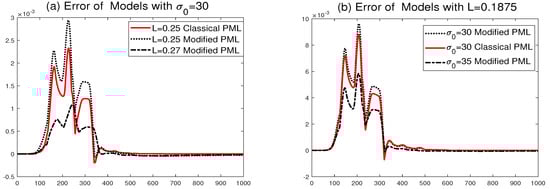
Figure 1. Comparison of errors: (a) a fixed damping ${\sigma }_0=30$, (b) a thickness $L=0.1875$ $(\beta =2)$.

To see the influence of absorbing property by incidence angle, we demonstrate both formulas with different positions of source function. The resulted differences between reference and computed values of the solution during simulation at one point within the computational domain are plotted in Figure 2. The errors of the classical PML have relatively smaller than the modified one and both formulas have slightly better absorbing property when the angle of incidence to the interface between the computational domain and the layers is bigger.

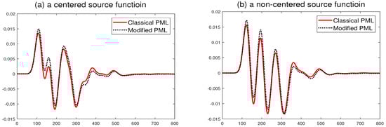
Figure 2. Comparison of the difference at a point from different positions of source function with ${\sigma }_0=35$ and $L=0.1$.

Next, to investigate the energy $\mathcal{E}(t)$ behavior, we choose a time step size $▵t$ of $▵x/3$, which satisfies the CFL condition (15) to guarantee the stability of the staggered finite difference scheme (see Remark 4). Here, the first order backward and second order central finite differences in time and space, respectively, are used to discretize the energy $\mathcal{E}(t_n)$ of (18) at each time step $t_n$. We investigate the behavior of the energy for a long-time simulation at time $t_n=$ 10,000 according to the thickness of the layers and magnitude of the damping. The numerical results are displayed in Figure 3: (a) the energy with various dampings ${\sigma }_0=40,50,50,60,70$ for a fixed thickness $L=0.0625$ and (b) the energy with various thicknesses $L=0.0625,0.1,0.125,0.15$ for a fixed damping ${\sigma }_0=50$. The results indicate that the numerical stability of the modified formula is consistently stable in the long-time simulation regardless of the magnitudes of damping and thickness of the layer. This provides proof of the well-posedness of the developed system and numerical stability for the finite difference method.

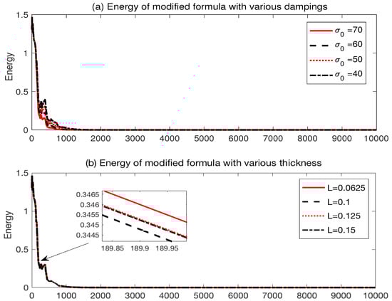
Figure 3. $\mathcal{E}(t)$ with (a) various damping values ${\sigma }_0=40,50,60,70$ for a fixed thickness $L=0.0625(\beta =0)$, (b) various thickness $L=0.0625,0.1,0.125,0.15$ for a fixed damping ${\sigma }_0=50(\beta =0)$.

Lastly, in order to illustrate this visual investigation, we consider the damping $\beta =2$ and display the snap shots of the wave propagation at times $t_n=1,30,60,100,130,150,200,300,500$ with ${\sigma }_0=35,L=0.25$ in Figure 4. One can see that the regularized system displays a good property of non-reflection in the layers, which is the purpose of building the layers. It is remarkable that from a mathematical point of view, the analytical well-posedness without losing the non-reflection property in the layers of that the classical PML model.

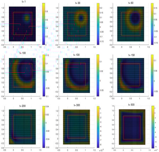
Figure 4. Snap shots of the regularized system at time $t_n=1,30,60,100,130,150,200,300,500$ with ${\sigma }_0=35,\beta =2,L=0.25$ (Red rectangular box represents the computational domain.)

5. Discussion

We have introduced a new and efficient formulation related to the acoustic wave equation based on the regularization of the un-split PML wave equation. By regularizing the lower order regularity term in the original equation and the standard von Neumann stability analysis, we have achieved well-posedness as well as numerical stability of the solution in the new formulation. We summarize the main novelty and results of this study as follows: (1) We have proved the analytical well-posedness of our formulation without any restriction of damping terms; (2) a staggered finite difference scheme for the formulation is introduced and numerical stability is also analyzed; (3) several numerical tests are exhibited to show the numerical stability and a non-reflection property.

References

- Bérenger, J.P. A perfectly matched layer for the absorption of electromagnetic waves. J. Comput. Phys. 1994, 114, 185–200. [Google Scholar] [CrossRef]
- Chew, W.C.; Weedon, W.H. A 3D Perfectly matched medium from modified Maxwell’s equations with stretched coordinates. Microw. Opt. Technol. Lett. 1994, 7, 599–604. [Google Scholar] [CrossRef]
- Sjögreen, B.; Petersson, N.A. Perfectly matched layers for Maxwell’s equations in second order formulation. J. Comput. Phys. 2005, 209, 19–46. [Google Scholar] [CrossRef]
- Collino, F.; Tsogka, C. Application of the PML absorbing layer model to the linear elastodynamic problem in anisotropic heterogeneous medias. Geophysics 2001, 88, 43–73. [Google Scholar]
- Chew, W.C.; Liu, Q.H. Perfectly matched layers for elastodynamics: A new absorbing boundary condition. J. Comput. Acoust. 1996, 4, 341–359. [Google Scholar] [CrossRef]
- Hu, F.Q. On absorbing boundary conditions for linearized Euler equations by a perfectly matched layer. J. Comput. Phys. 1996, 129, 201–219. [Google Scholar] [CrossRef]
- Hesthaven, J.S. On the analysis and construction of perfectly matched layers for the linearized Euler equations. J. Comput. Phys. 1998, 142, 129–147. [Google Scholar] [CrossRef]
- Lions, J.-L.; Métral, J.; Vacus, O. Well-posed absorbing layer for hyperbolic problems. Numer. Math. 2002, 92, 535–562. [Google Scholar] [CrossRef]
- Nataf, F. A new approach to perfectly matched layers for the linearized Euler system. J. Comput. Phys. 2006, 214, 757–772. [Google Scholar] [CrossRef]
- Turkei, E.; Yefet, A. Absorbing PML boundary layers for wave-like equations. Appl. Num. Math. 1998, 27, 533–557. [Google Scholar] [CrossRef]
- Barucq, H.; Diaz, J.; Tlemcani, M. New absorbing layers conditions for short water waves. J. Comput. Phys. 2010, 229, 58–72. [Google Scholar] [CrossRef]
- Appelö, D.; Hagstrom, T.; Kress, G. Perfectly matched layer for hyperbolic systems: General formulation, well-posedness, and stability. J. Appl. Math. 2006, 67, 1–23. [Google Scholar] [CrossRef]
- Hu, F.Q. A stable perfectly matched layer for linearized Euler equations in unsplit physical variables. J. Comput. Phys. 2001, 173, 455–480. [Google Scholar] [CrossRef]
- Cohen, G.C. Higher-Order Numerical Methods for Transient Wave Equations; Springer: Berlin, Germany, 2002. [Google Scholar]
- Zhao, L.; Cangellaris, A.C. A general approach for the development of unsplit-field time-domain implementations of perfectly matched layers for FDTD grid truncation. IEEE Microw. Guided Lett. 1996, 6, 209–211. [Google Scholar] [CrossRef]
- Bécache, E.; Joly, P. On the analysis of Bérenger’s Perfectly Matched Layers for Maxwell’s equations. Math. Model. Numer. Anal. 2002, 36, 87–120. [Google Scholar] [CrossRef]
- Abarbanel, S.; Gottlieb, D. A mathematical analysis of the PML method. J. Comput. Phys. 1997, 134, 357–363. [Google Scholar] [CrossRef]
- Halpern, L.; Petit-Bergez, S.; Rauch, J. The analysis of matched layers. Conflu. Math. 2011, 3, 159–236. [Google Scholar] [CrossRef]
- Abarbanel, S.; Qasimov, H.; Tsynkov, S. Long-time performance of unsplit PMLs with explicit second order schemes. J. Sci. Comput. 2009, 41, 1–12. [Google Scholar] [CrossRef]
- Roden, J.A.; Gedney, S.D. Convolution PML (CPML): An efficient FDTD implementation of the CFS–PML for arbitrary media. Microw. Opt. Technol. Lett. 2000, 27, 334–339. [Google Scholar] [CrossRef]
- Rylander, T.; Jin, J. Perfectly matched layer for the time domain finite element method. J. Comput. Phys. 2004, 200, 238–250. [Google Scholar] [CrossRef]
- Komatitsch, D.; Tromp, J. A perfectly matched layer absorbing boundary condition for the second-order seismic wave equation. Geophys. J. Int. 2003, 154, 146–153. [Google Scholar] [CrossRef]
- Appelö, D.; Kress, G. Application of a perfectly matched layer to the nonlinear wave equation. Wave Motion 2007, 44, 531–548. [Google Scholar] [CrossRef]
- Tam, C.K.W.; Auriault, L.; Cambuli, F. Perfectly matched layer as absorbing condition for the linearized Euler equations in open and ducted domains. J. Comput. Phys. 1998, 114, 213–234. [Google Scholar] [CrossRef]
- Diaz, J.; Joly, P. A time domain analysis of PML models in acoustics. Comput. Methods Appl. Mech. Eng. 2006, 195, 3820–3853. [Google Scholar] [CrossRef]
- Johnson, S. Notes on Perfectly Matched Layers; Technical Report; Massachusetts Institute of Technology: Cambridge, MA, USA, 2010. [Google Scholar]
- Hagstrom, T.; Hariharan, S.I. A formulation of asymptotic and exact boundary conditions using local operators. Appl. Numer. Math. 1998, 27, 403–416. [Google Scholar] [CrossRef]
- Grote, M.J.; Sim, I. Efficient PML for the wave equation. arXiv, 2010; arXiv:1001.0319v1. [Google Scholar]
- Bécache, E.; Petropoulos, P.G.; Gedney, S.D. On the long-time behavior of unsplit perfectly matched layers. IEEE Trans. Antennas Propag. 2004, 52, 1335–1342. [Google Scholar] [CrossRef]
- Petersen, B.E. Introduction to the Fourier Transform and Pseudo-Differential Operators; Series: Monographs and studies in mathematics; Pitman Advanced Pub. Program: Boston, MA, USA, 1983. [Google Scholar]
- Kim, D. The Variable Speed Wave Equation and Perfectly Matched Layers. Ph.D. Thesis, Oregon State University, Corvallis, OR, USA, 2015. [Google Scholar]
- Evans, L.C. Partial Differential Equations, 2nd ed.; Graduate Series in Mathematics; Springer: Berlin, Germany, 2010. [Google Scholar]
- LeVeque, R.J. Finite Difference Methods for Ordinary and Partial Differential Equations; Society for Industrial and Applied Mathematics: Philadelphia, PA, USA, 2007. [Google Scholar]
- Trucco, E.; Verri, A. Introductory Techniques for 3-D Computer Vision; Prentice Hall: Upper Saddle River, NJ, USA, 1998. [Google Scholar]
- Bidégaray-Fesquet, B. Stability of FD-TD schemes for Maxwell-Debye and Maxwell-Lorentz equations. SIAM J. Numer. Anal. 2008, 46, 2551–2566. [Google Scholar] [CrossRef]
- Miller, J.J.H. On the location of zeros of certain classes of polynomials with applications to numerical analysis. J. Inst. Math. Appl. 1971, 8, 397–406. [Google Scholar] [CrossRef]
- Kaltenbacher, B.; Kaltenbacher, M.; Sim, I. A modified and stable version of a Perfectly Matched Layer technique for the 3-d second order wave equation in time domain with an application to aeroacoustics. J. Comput. Phys. 2013, 35, 407–422. [Google Scholar] [CrossRef]
© 2019 by the author. Licensee MDPI, Basel, Switzerland. This article is an open access article distributed under the terms and conditions of the Creative Commons Attribution (CC BY) license (http://creativecommons.org/licenses/by/4.0/).