Robust CFAR Detection for Multiple Targets in K-Distributed Sea Clutter Based on Machine Learning

Abstract

For K-distributed sea clutter, a constant false alarm rate (CFAR) is crucial as a desired property for automatic target detection in an unknown and non-stationary background. In multiple-target scenarios, the target masking effect reduces the detection performance of CFAR detectors evidently. A machine learning based processor, associating the artificial neural network (ANN) and a clustering algorithm of density-based spatial clustering of applications with noise (DBSCAN), namely, DBSCAN-CFAR, is proposed herein to address this issue. ANN is trained with a symmetrical structure to estimate the shape parameter of background clutter, whereas DBSCAN is devoted to excluding interference targets and sea spikes as outliers in the leading and lagging windows that are symmetrical about the cell under test (CUT). Simulation results verified that the ANN-based method provides the optimal parameter estimation results in the range of 0.1 to 30, which facilitates the control of actual false alarm probability. The effectiveness and robustness of DBSCAN-CFAR are also confirmed by the comparisons of conventional CFAR processors in different clutter conditions, comprised of varying target numbers, shape parameters, and false alarm probabilities. Although the proposed ANN-based DBSCAN-CFAR processor incurs more elapsed time, it achieves superior CFAR performance without a prior knowledge on the number and distribution of interference targets.

1. Introduction

With the development of radar resolution, numerous studies have shown that the amplitude distribution of a sea clutter exhibits a long tail appreciably [1,2]. At this time, the traditional Rayleigh, Weibull, and log-normal distributions cannot describe the statistical characteristics of sea clutter adequately; therefore, the K-distribution has been introduced for the modeling and simulation of high-resolution sea clutters [3,4]. In K-distribution model, it is assumed that the amplitude of sea clutter in each range unit obeys Rayleigh distribution (also known as speckle component), and its intensity obeys gamma distribution (i.e., texture component). Different from the previous distribution model, the K-distribution model can be reasonably explained from the scattering mechanism of a clutter, and its effectiveness has been supported and verified by experimental data in practical applications [5].

Detecting targets is the fundamental task of a radar system. As an effective method for target detection, the constant false alarm rate (CFAR) technology can maximize the detection probability while maintaining a constant false alarm probability [6,7]. In previous studies, several types of CFAR processors have been proposed based on the mechanism of a sliding reference window. They perform statistical analysis on the clutter background, calculate dynamic thresholds, and make a comparison with the cell under test (CUT) to realize automatic detection of the targets. The most well-known processors encompass cell averaging CFAR (CA-CFAR) [8], greatest-of CFAR (GO-CFAR) [9], and smallest-of CFAR (SO-CFAR) [10], which are collectively called the mean-level processors. However, when they are applied to a complex background such as K-distributed sea clutter, the optimal detection performance may not be achieved, especially in the case of multiple targets. If one or more interference targets fall within the reference window, the probability of losing the targets will be increased owing to the severe phenomenon of target masking. To mitigate this adverse effect, a feasible solution is to develop a more accurate estimation strategy for the clutter background level. Consequently, following the mean-level processors, a class of sorting-based processors are also applied to CFAR detection, such as ordered statistics CFAR (OS-CFAR) [11] and censored mean level detector CFAR (CMLD-CFAR) [12]. They sort the sample values of the reference window in ascending order, and then select the specific rank-ordered reference cell by a preset parameter or exclude a part of the high-amplitude reference cells to represent the average power of the clutter. In this way, the interference targets and sea spikes in the reference window will be removed as outliers when estimating the background level. The detection performance of sorting-based processors is better than CA, SO, and GO-CFAR in multiple-target scenarios; however, they rely heavily on a priori information about the number and distribution of interference targets.

Furthermore, some new detection algorithms for multiple-target situations have emerged in succession. The variability index CFAR (VI-CFAR) detector [13] determined the uniformity of the background clutter by calculating the second moment and the mean of the reference window, and adaptively selected CA, SO, and GO to estimate the background power. However, when the background clutter has a complicated distribution, the detection performance will suffer from inevitable degradation. In [14], a CATM-CFAR detector combining cell-averaging and trimmed mean CFAR was presented for a software defined radar in both the simulated Weibull clutter and real clutter. In [15], they proposed a truncated statistic CFAR (TS-CFAR) for ship detection in single-look intensity and multilook intensity synthetic aperture radar (SAR) data. It utilizes the method of truncation to remove the possible interference outliers in multiple-target situations. In [16], a novel CFAR detector adopted the weighted amplitude iteration of the samples in the reference window as an adaptive threshold for target detection in nonhomogeneous, gamma-distributed clutter.

As a multidisciplinary subject, machine learning [17] has received extensive attention in recent years. Relevant technologies in machine learning, such as artificial neural networks (ANN), deep learning, and clustering algorithms [18], have been applied to many research fields [19,20,21]. Among these technologies, ANN is the most dazzling one. In [22], the method of ANN was introduced to classify the sea clutter preferential distribution for achieving faster and more precise results than the traditional alternative. In [23], they addressed the task of ship discrimination by using a very deep network configuration in SAR sensors. In [24], they proposed a neural network detector with partial CA-CFAR supervised training for fluctuating Swerling targets. More generally, ANNs are widely used in parameter estimation of different distributed clutters, such as Weibull distribution [25], Pareto distribution [26], and K-distribution [27,28]. Other for ANN, another important technique in the field of machine learning is the clustering algorithm, involving k-means, an isolation forest, local outlier factor (LOF), and density-based spatial clustering of applications with noise (DBSCAN) [29,30,31]. Although outstanding in data mining, clustering algorithms are also suitable for radar target detection in non-uniform clutter backgrounds. In [32], a modified CA-CFAR was presented based on Grubbs criterion for multiple-target scenarios. However, the Grubbs criterion is applicable only to detective a single outlier in a univariate dataset that follows an approximately normal distribution. This limitation prevents it from being utilized in a K-distribution clutter for reaching the optimal detection performance. At present, there are few studies using clustering algorithms to address the problem of multiple-target CFAR detection in K-distributed sea clutter.

The purpose of this paper is to improve the detection performance affected by target masking effect in multitarget scenarios for K-distributed sea clutter. By associating the advantages of ANN and DBSCAN, a machine learning based CFAR processor is proposed in this paper. The main contributions are summarized as follows:

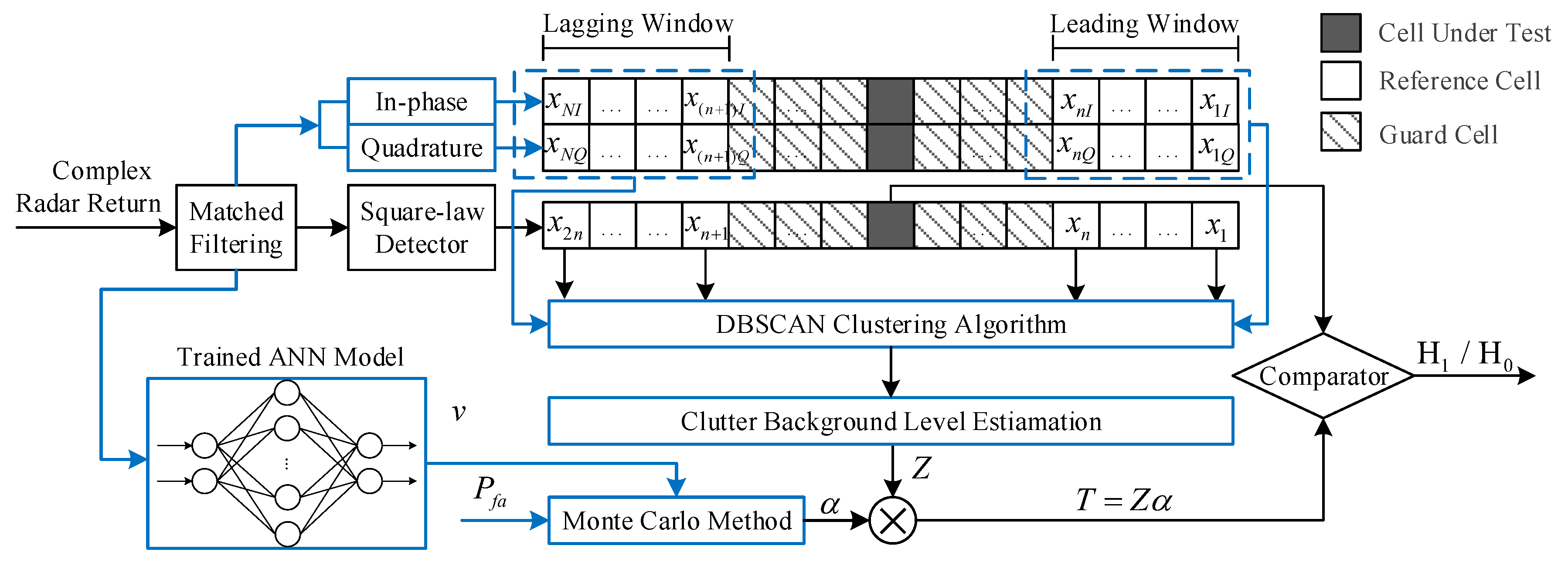
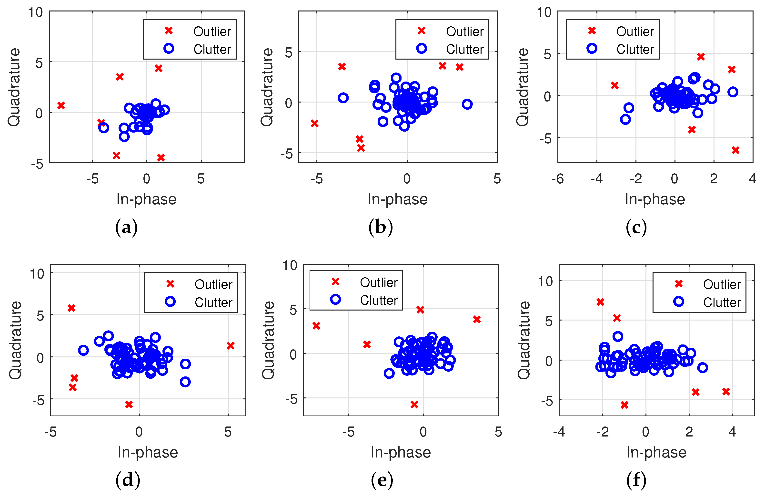
• We propose a novel CFAR processor based on the DBSCAN clustering algorithm, termed DBSCAN-CFAR, to eliminate outliers in the leading and lagging windows that are symmetrical about the CUT. Without a priori knowledge on the number and distribution of interference targets, the DBSCAN-CFAR can achieve an accurate estimation of the clutter background level for multiple-target scenarios. The configuration parameters of DBSCAN are predetermined according to the characteristics of the clutter data to ensure real-time performance of the detector.
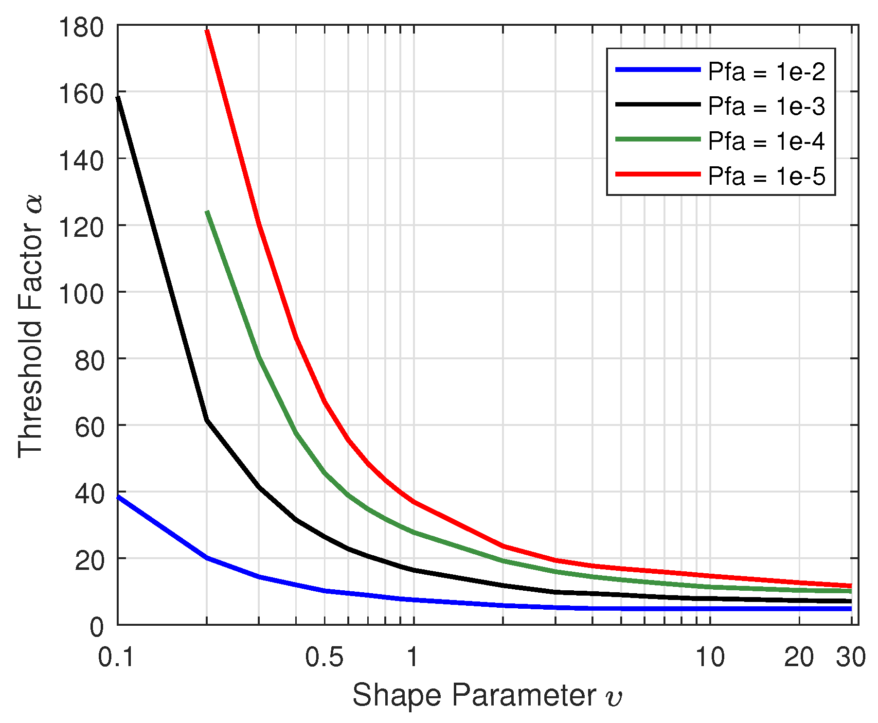
• We design and train an ameliorative ANN model with a symmetrical architecture to evaluate the shape parameter of K-distributed sea clutter with high precision. Through deriving the numerical relationship between the threshold factor and the shape parameter under different false alarm probabilities, the optimal parameter estimation value offered by the ANN method is instrumental in maintaining the CFAR property for DBSCAN-CFAR.
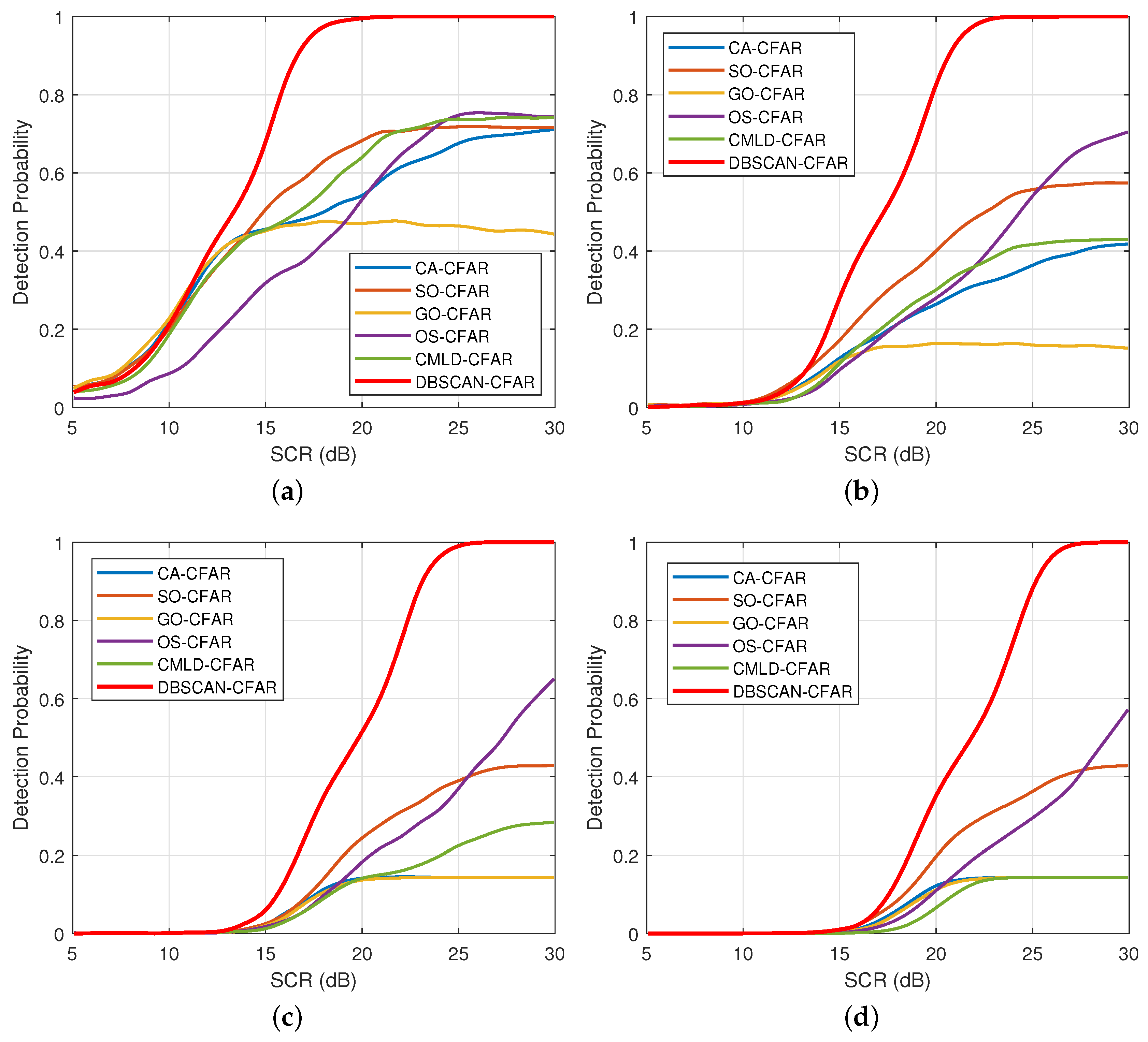
• We demonstrate the effectiveness and superiority of the proposed ANN-based DBSCAN-CFAR processor over several relevant competitors with respect to the variation of interference target numbers, shape parameters, and false alarm probabilities through extensive simulations. This performance improvement is at the expense of time that elapses.

The paper is organized as follows. Section 2 elucidates the concepts of K-distributed sea clutter model, CFRA detection, and shape parameter estimation. In Section 3, the implementations of DBSCAN-CFAR and the ANN model are provided in detail. The detection performance of the proposed ANN-based DBSCAN-CFAR processor is compared and analyzed in Section 4. Finally, Section 5 presents the main conclusions of this paper.

2. Preliminary Theories

In this section, we briefly introduce the K-distributed sea clutter model, CFAR detection, and shape parameter estimation, which serve as the precursors of our proposal.

2.1. K-Distributed Sea Clutter Model

In the K-distributed model, sea clutter signal X is usually considered the product of two independent components, given by:

$$X=\sqrt{X_G}·X_R=Y·X_R,$$

(1)

where $X_G$ and $X_R$ denote the texture component and speckle component respectively. Among them, $Y=\sqrt{X_G}$ follows the generalized $\chi$ distribution, whose probability density function (PDF) is:

$$f\left(y\right)=\frac{2c^{2v}{y}^{2v-1}}{\mathsf{\Gamma }\left(v\right)}\exp \left(-c^2{y}^2\right),y>0,$$

(2)

where $\mathsf{\Gamma }(·)$ is the gamma function, and v and c are the shape parameter and scale parameter, respectively. Obeying the Rayleigh distribution, the PDF of $X_R$ can be obtained by:

$$f\left(x\right|y)=\frac{x\pi }{2y^2}\exp \left(-\frac{x^2\pi }{4y^2}\right),x>0.$$

(3)

Consequently, the PDF of the K-distributed sea clutter can be expressed as follows [33]:

$$f_K\left(x\right)={\int }_0^{+\infty }f\left(x\right|y)f\left(y\right)dy=\frac{2c}{\mathsf{\Gamma }\left(v\right)}{\left(\frac{cx}{2}\right)}^v{K}_{v-1}\left(cx\right),$$

(4)

where v represents the shape parameter and its value range belongs to $0.1\le v<\infty$, reflecting the spikiness of sea clutter. $c>0$ is the scale parameter, which relates to the average power of sea clutter. Besides, $K_{v-1}(·)$ is the modified Bessel function of the second kind with order $v-1$.

2.2. CFAR Detection

For a CFAR processor, the main purpose is to determine the presence or absence of the target in a radar echo signal with interferences by setting a dynamic threshold. Specifically, this dynamic threshold is inseparable from the desired false alarm probability and the estimated clutter background level.

As shown in Figure 1, the complex radar return signal with in-phase and quadrature components, after matched filtering, is processed by square-law, and the successive outputs are run through a sliding window, which consists of reference cells, guard cells, and the CUT. Assume the samples of the reference cells are $\{x_1,x_2,\dots ,x_n\}$ in the leading window and $\{x_{n+1},x_{n+2},\dots ,x_{2n}\}$ in the lagging window, wherein $N=2n$ refers to the length of the reference window. The leading window and the lagging window are symmetrical with respect to the CUT. Due to the spatial-temporal correlation of the radar echo, it is reasonable to employ the surrounding reference cells of the CUT for estimating the clutter background level. Besides, to remove the influence of the extended target in the CUT on this estimating process, a small number of guard cells are arranged adjacent to both sides of the CUT in some CFAR processors, such as CA, GO, and SO-CFAR. With the samples in the reference window, the clutter background level of the CUT (labeled as Z) can be evaluated based on different detection schemes. For instance, several typical representatives of mean-level and sorting-based processors are described as following:

$$\{\begin{array}{}\mathrm{(5)}& Z_{CA}=\frac{1}{N}{\displaystyle \sum _{i=1}^{2n}}{x}_i\hfill \mathrm{(6)}& Z_{GO}=\max \left(\frac{2}{N}{\displaystyle \sum _{i=1}^n}{x}_i,\frac{2}{N}{\displaystyle \sum _{i=n+1}^{2n}}{x}_i\right)\hfill \mathrm{(7)}& Z_{SO}=\min \left(\frac{2}{N}{\displaystyle \sum _{i=1}^n}{x}_i,\frac{2}{N}{\displaystyle \sum _{i=n+1}^{2n}}{x}_i\right)\hfill \mathrm{(8)}& Z_{OS}=x_{\left(k\right)},x_{\left(1\right)}\le x_{\left(2\right)}\le \cdots \le x_{\left(k\right)}\le \cdots \le x_{\left(N\right)},k\le N\hfill \mathrm{(9)}& Z_{CMLD}=\frac{1}{N-r}{\displaystyle \sum _{i=1}^{N-r}}{x}_{\left(i\right)},x_{\left(1\right)}\le x_{\left(2\right)}\le \cdots \le x_{(r-1)}\le x_{\left(r\right)}\le \cdots \le x_{\left(N\right)},r<N.\hfill \end{array}$$

After that, the detection threshold T can be calculated by multiplying the estimated clutter background level Z by a threshold factor $\alpha$, namely:

$$T=\alpha Z.$$

(10)

Finally, the actual value of the CUT (labeled as $x_0$) and the detection threshold T are passed through a comparator to obtain the detection result. The decision criteria boils down to a testing of binary hypothesis:

$$x_0{\displaystyle \underset{H_0}{\overset{H_1}{\gtrless }}}T,$$

(11)

where the hypothesis $H_1$ indicates the presence of a target in current CUT, and $H_0$ indicates the absence.

In multiple-target environments, the statistical characteristics of interference targets are usually different from those of sea clutter background. Besides, the existence of sea spikes can also adversely affect estimating the clutter background level. Figure 2 presents a typical multiple-target scenario in K-distributed sea clutter. As shown, the Neyman–Pearson threshold is no longer applicable because it causes many undesired false alarms. Despite that the CFAR threshold can avoid this drawback, multiple targets densely distributed in the range domain may produce target masking effect, which makes low power targets unable to be detected correctly. To obtain an accurate estimation result for the clutter background level, these negative factors of interference targets and sea spikes need to be excluded from the reference window, and then the detection threshold is computed based on the remaining reference cells. Due to the detection schemes, several processors of SO, OS, and CMLD-CFAR can handle this problem to a certain extent for multiple-target detection. However, these methods require a priori information about the number and distribution of interference targets. In practice, this information is generally random and unpredictable before detecting. Consequently, a robust processor without a priori knowledge will be more applicable for adaptive CFAR detection in multiple-target scenarios.

2.3. Shape Parameter Estimation

Note that in Equation (4), the shape parameter v plays an important role in K-distributed sea clutter model, which determines the tail of clutter amplitude distribution. Moreover, the detection threshold of most adaptive CFAR processors is dependent on the shape parameter and the estimated clutter background level. For a fixed false alarm probability, the variation of the shape parameter has a major impact on the threshold factor. If they are mismatched, it will lead to undesired missed detection or excessive false alarms. The previous discussion assumes that the shape parameter is exactly known. Nevertheless, this parameter is actually unknown and needs to estimate from the sea clutter data. Therefore, accurate estimation of the shape parameter is particularly an imperative prerequisite for effectively improving the target detection performance.

In past research, numerous methods have been proposed for shape parameter estimation, such as maximum likelihood estimation (MLE) [34,35,36] and method of moments (MOM) [37,38,39]. Since K-distribution is no longer an ordinary elementary function, it is quite complex to apply the MLE method to solve the distribution parameters, which results in a huge amount of computation. By contrast, the MOM method makes the theoretical moments of the clutter distribution function equal to the experimental moments, and then seeks the corresponding parameters through mathematical equations. Benefiting from the simple principle and operation, this approach can greatly reduce the computational complexity. Therefore, we only introduce the most commonly used MOM method here.

For a K-distributed model, the origin moments of all orders exist theoretically. Supposing the t-th moment can be defined as:

$${\mu }_t=E\left(X^t\right)=\frac{\mathsf{\Gamma }(v+0.5t)\mathsf{\Gamma }(1+0.5t)}{\mathsf{\Gamma }\left(v\right)}{\left(2c\right)}^t,t\ge 0.$$

(12)

In general, the methods of the first-order/second-order algebraic moment (abbreviated as MOM-12) and second-order/fourth-order algebraic moment (abbreviated as MOM-24) are utilized to estimate the unknown parameters of K-distribution, given by:

$$\left\{\begin{array}{c}\frac{{\widehat{\mu }}_1^2}{{\widehat{\mu }}_2}=\frac{{\mathsf{\Gamma }}^2(1+0.5){\mathsf{\Gamma }}^2(\widehat{v}+0.5)}{\widehat{v}{\mathsf{\Gamma }}^2\left(\widehat{v}\right)}\hfill \\ \widehat{c}=\frac{{\widehat{\mu }}_1\mathsf{\Gamma }\left(\widehat{v}\right)}{\sqrt{\pi }\mathsf{\Gamma }(\widehat{v}+0.5)},\hfill \end{array}\right.$$

(13)

$$\left\{\begin{array}{c}\widehat{v}={\left(\frac{{\widehat{\mu }}_4}{2{\widehat{\mu }}_2^2}-1\right)}^{-1}\hfill \\ \widehat{c}=\frac{1}{2}\sqrt{\frac{{\widehat{\mu }}_2}{\widehat{v}}},\hfill \end{array}\right.$$

(14)

where $\widehat{v}$ and $\widehat{c}$ are the estimated shape and scale parameters respectively. It is worth mentioning that, although the MOM methods can overcome the shortcoming of massive computation in MLE, they sacrifice a certain estimation accuracy. Moreover, the high-order moments are sensitive to the clutter data, which is unfavorable for parameter estimation.

3. Proposed Methods

As mentioned in Section 1, our machine learning based processor accomplishes the process of CFAR detection in two parts. For one part, we train an ANN model to evaluate the shape parameter of sea clutter accurately for maintaining the CFAR property. In the other part, we apply the DBSCAN algorithm to get a precise estimation for the clutter background level by restraining the effect of interference targets and sea spikes, and then obtain the verdict of the CFAR detector. More details of these two parts are provided in the subsequent two subsections, respectively.

3.1. DBSCAN-CFAR Processor

As a prevalent, density-based clustering algorithm in the area of machine learning, DBSCAN [29,30,31] can generate arbitrarily shaped clusters based on two parameters; i.e., the neighborhood radius $Eps$ and the minimum number of points in this neighborhood $MinPts$. It performs attractively in dealing with complex and irregular data, especially in outlier detection. Different from the K-means algorithm, DBSCAN does not require a specified number of clusters in advance, in which the potential relationship between the normal data and outliers can be learned without labels. The mathematical definitions and principles of the DBSCAN algorithm [40,41] will be elaborated in the following part.

Assuming in a data set of D, the neighborhood radius $Eps$ of a point p is defined as:

$$N_{Eps}\left(p\right)=\{p,q\in D\mid dist(p,q)\le Eps\},$$

(15)

where $dist(p,q)$ represents the Euclidean distance between the point p and point q. As shown in Figure 3, if the point p contains at least $MinPts$ other points within its $Eps$-neighborhood, it will be defined as a core point by:

$$p=\{p\in D\mid \parallel N_{Eps}\left(p\right)\parallel \ge MinPts\}.$$

(16)

In contrast, if a non-core point falls within the neighborhood of core points but the number of other points in its radius $Eps$ is less than $MinPts$, it will be termed a border point by:

$$q=\{p\in D,q\in N_{Eps}\left(p\right)\mid \parallel N_{Eps}\left(q\right)\parallel <MinPts\}.$$

(17)

Except for the core points and border points, the remaining points in the data set are regarded as outliers. It implies that outliers belong to the data set of D, but not to any clusters, as follows:

$$p=\{p\in D\mid \forall i:p\notin C_i\},$$

(18)

where $C_i,i=1,2,\cdots ,k$ denotes the k clusters generated.

According to the fundamental concepts, if a point p lies in the $Eps$-neighborhood of a core point q, it will be called directly density-reachable from q; i.e., satisfying the following condition as:

$$\{p,q\in D,p\in N_{Eps}\left(q\right)\mid \parallel N_{Eps}\left(q\right)\parallel \ge MinPts\}.$$

(19)

Specifically, if there is a series of points $p_i\in D,i=1,2,\cdots ,n$ with $p_1=q$ and $p_n=p$, and it is directly density-reachable from $p_i$ to $p_{i+1}$, the point p will be so-called density-reachable from a core point q with respect to the parameters of $Eps$ and $MinPts$, as depicted in Figure 3. Moreover, if there is a point $g\in D$ enables that the points of p and q are both density-reachable from g, two points of p and q are density-connected with $Eps$ and $MinPts$. By starting from any core point, all density-reachable points can be gathered to a cluster. After clustering, the pending data are categorized into core points, border points, and outliers. As a result, the density of a cluster covering core points and border points will be greater than that of outliers. Benefiting from this feature, the DBSCAN algorithm is able to distinguish the high-density clusters and low-density outliers automatically.

Motivated by the mentioned advantages, the DBSCAN algorithm is introduced into the multiple-target detection for K-distributed sea clutter. Since the potential targets and sea spikes are usually different from the background clutter in statistics, it is reasonable to regard them as outliers in sea clutter. In this paper, a novel CFAR processor is proposed based on the DBSCAN algorithm; namely, DBSCAN-CFAR. The block diagram of this processor is illustrated in Figure 4. The DBSCAN-CFAR retains the original framework of the conventional CFAR processor and incorporates the operations of outlier rejection into the detection process. As highlighted in blue, these are two main differences compared with the processors in Figure 1. On the one hand, the in-phase and quadrature components of the complex radar return are adopted to assist in detecting outliers through the DBSCAN algorithm. It is established on such a basis that, if the two components of the complex signal present as an outlier, the signal amplitude will still behave as an outlier after square-law detection. On the other hand, the threshold factor $\alpha$ here is derived from the estimated shape parameter v using a trained ANN model and the desired false alarm probability $P_{fa}$, whereas $\alpha$ is generally given as an closed-form solution for traditional CFAR processors in Rayleigh-distributed clutter. By censoring the outliers in reference windows, the proposed DBSCAN-CFAR processor can effectively improve the estimation accuracy of the clutter background level and promote the detection performance.

As shown in Figure 4, suppose that in the range of a reference window, the complex echo signal received by the radar is expressed as:

$$\mathbf{X}=\left[x_{1I}+j{x}_{1Q},x_{2I}+j{x}_{2Q},\dots ,x_{NI}+j{x}_{NQ}\right],$$

(20)

where $N=2n$ stands for the length of the reference window. Besides, after the sample of each range unit passes through the square law detector, the corresponding signal can be given as:

$$x_i=x_{iI}^2+x_{iQ}^2,$$

(21)

where $i=1,2,\dots ,N$.

During the detection process, our DBSCAN-CFAR processor first utilizes the clustering algorithm to distinguish normal data points and outliers from N samples of the complex signal X. If the subscript of an outlier in X is s, the sample $x_s$ corresponding to the subscript value in the signal $x_i$ is also an outlier. Therefore, the clutter background level of CUT can be estimated by removing these outliers from $x_i$ and averaging the remaining samples, as follows:

$$Z_{DBSCAN}=\frac{1}{N-S}{\displaystyle \sum _{i=1}^{N-S}}\left\{x_i\backslash x_s\right\},i=1,2,\dots ,N,s\in [1,N],$$

(22)

where S is the number of outliers separated by clustering algorithm.

After that, take $Z_{DBSCAN}$ into Equations (10) and (11) to establish the detection scheme for DBSCAN-CFAR processor, given by:

$$x_0{\displaystyle \underset{H_0}{\overset{H_1}{\gtrless }}}\frac{\alpha }{N-S}{\displaystyle \sum _{i=1}^{N-S}}\left\{x_i\backslash x_s\right\},i=1,2,\dots ,N,s\in [1,N],$$

(23)

where $x_0$ and $\alpha$ denote the actual values of CUT and the threshold factor respectively.

Given these ingredients, the detailed pseudo code of the DBSCAN-CFAR processor is exhibited in Algorithm 1.

Algorithm 1 Proposed DBSCAN-CFAR Processor

Input: Number of reference cells N, number of guard cells M, complex samples of radar return in reference window $\left[x_{1I}+j{x}_{1Q},\cdots ,x_{NI}+j{x}_{NQ}\right]$, and clustering parameters of $Eps$ and $MinPts$. Output: Target detection result ($H_1$ or $H_0$). 1: Initialize the set of a cluster $\mathsf{\Omega }=⌀$. 2: Extract the quadrature and in-phase components of each complex sample to form a two-dimensional point set as $D=\left\{(x_{1I},x_{1Q}),\dots ,(x_{NI},x_{NQ})\right\}$. 3: for each point $p\in D$ do 4:   if p is checked 5:    Continue for next point. 6:   else 7:    Count the number of all points within the $Eps$-neighborhood for point p as $\parallel N_{Eps}\left(p\right)\parallel$. 8:    if ($\parallel N_{Eps}\left(p\right)\parallel <MinPts$) 9:    Mark p as a border point or outlier. 10:    else 11:    Mark p as a core point and classify the all points in its $Eps$-neighborhood to the cluster $\mathsf{\Omega }$. 12:    for an unchecked point q in the $Eps$-neighborhood of point p do 13:     if ($\parallel N_{Eps}\left(q\right)\parallel \ge MinPts$) 14:     Add the unchecked points within the neighborhood of point q into the cluster $\mathsf{\Omega }$. 15:     end if; 16:    end for; 17:    end if; 18:   end if; 19: end for; 20: Return the clustering result of DBSCAN, including outliers and normal clutter samples. 21: Calculate the clutter background level $Z_{DBSCAN}$ based on Equation (22). 22: Determine the target detection result as $H_1$ or $H_0$ according to Equation (23).

In light of the aforementioned discussion, the DBSCAN algorithm requires two parameters of $Eps$ and $MinPts$ to be determined, which refer to the value of neighborhood radius and the minimum number of points in the neighborhood, respectively. Since DBSCAN is integrated into the proposed CFAR processor, we also need to specify these two parameters before deployment. For the value of $MinPts$, previous studies have revealed that it should not be too large or too small on account of generating small clusters and reducing the influence of outliers. Generally, $MinPts=4$ is considered appropriate for two-dimensional data [40]. For the other parameter $Eps$, underlying the original work in [40], many approaches have been proposed to determine this parameter, such as normalized density list [42], histogram equalization [30], and improved multi-verse optimizer algorithm [43].

As a matter of fact, the real-time detection performance of a CFAR processor is a factor worthy of attention. To avoid introducing more computational complexity and ensure the real-time performance, we determine the value of the parameter $Eps$ based on the characteristics of sea clutter data by a larger number of repeated experiments. In this paper, the evaluation criterion of F-measure [44] is employed to quantitate the clustering results intuitively. Related with the ideas of precision rate P and recall rate R from the information retrieval, the F-measure is defined as the weighted harmonic mean of P and R, given by:

$$\mathrm{F}-\mathrm{measure}=\frac{({\beta }^2+1)·P·R}{{\beta }^2·P+R},$$

(24)

where ${\beta }^2\in [0,\infty ]$ and it is chosen as $\beta =1$ to balance the equal weights for P and R in this paper. The larger the F-measure is, the higher the quality of clustering result is. More about F-measure can be found in [44].

Figure 5 depicts the clustering quality of DBSCAN algorithm with different $Eps$ and $MinPts$ values. As shown, for a fixed $MinPts$, each curve presents an upward trend with the varying $Eps$ from 0.5 to 2, but gradually declines in the range from 2 to 5. It is evident that three curves have the similar clustering quality on the whole, and all of them obtain the optimal value of F-measure at $Eps=2$. Since the clustering results are not very insensitive to the value of $MinPts$, we selected $MinPts=4$ in our DBSCAN-CFAR processor to coincide with [40].

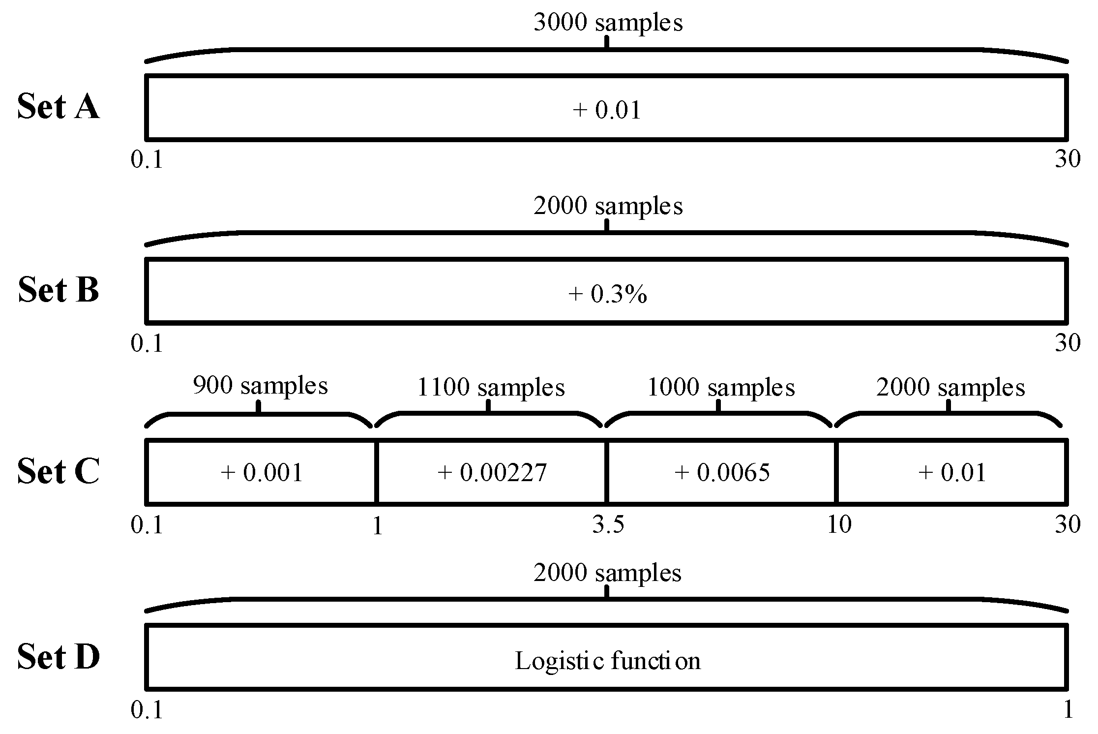
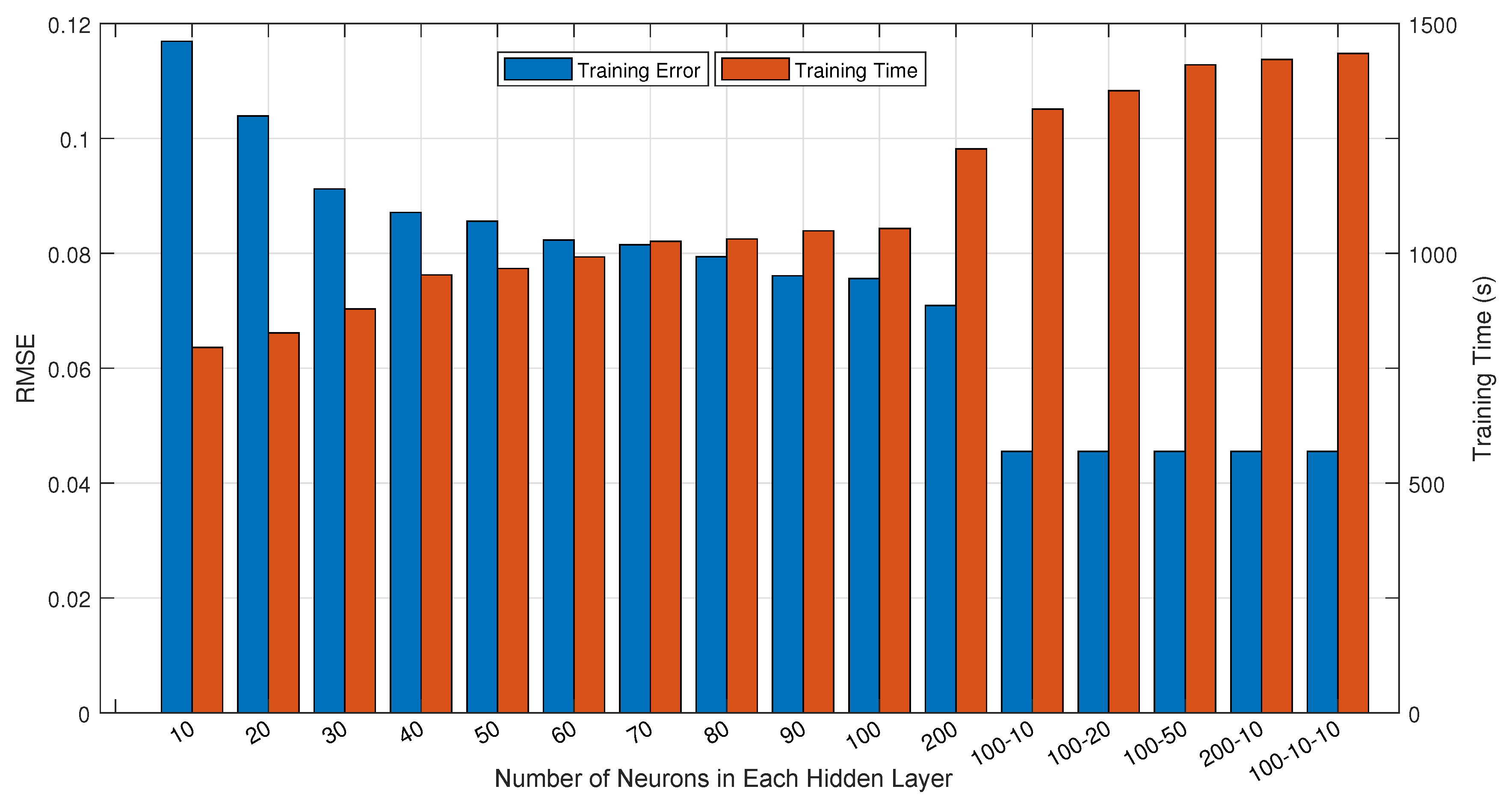
3.2. ANN-Based Shape Parameter Estimation

As shown in Figure 4, the shape parameter v of K-distributed sea clutter is estimated by a trained ANN model in our work. Particularly, ANN imitates the structure of human brain with interconnected neurons and presents powerful capabilities of self-learning, adapting, and organizing with information from external environments. This feature makes it highly applicable to solving the complicated nonlinear problems, including the shape parameter estimation of K-distribution that we are concerned about now.

In principle, using an ANN model to address this issue comprises two stages of offline training and online working successively. First of all, massive training data are required to be prepared for training the ANN model. To distinguish the sea clutters with different shape parameters, the histograms of radar return samples are extracted as the training data. Without loss of generality, the scale parameter of K-distribution is maintained with $c=v$ to fix the average power of the samples to one in all simulations. For each shape parameter, a quantity of 5000 samples generated by computer simulations are adopted to construct the histogram with 50 equispaced bins. Note that a portion of these simulated data contain a small number of targets with random intensities and positions to imitate the real environments. Here, we aim to examine the most practical shape parameter varying within the range of [0.1, 30] for K-distributed sea clutter [27,45].

Since the shape parameter reflects the sharpness of the sea clutter, the smaller the shape parameter, the greater its influence on the trailing of K-distribution is. It is challenging to train and evaluate the small shape parameters in neural networks. Consequently, when preparing the training data, it is reasonable to configure more training samples with small shape parameters and fewer samples with large parameters, which can ensure training accuracy and avoid redundant training. To realize this purpose, different segmentation methods are utilized to divide the shape parameters into four different training sets. As shown in Figure 6, Set A is uniformly distributed from 0.1 to 30 at the interval of 0.01, and Set B is increased gradually with a growth rate of 0.3%. Besides, Set C is applied with varying intervals for different partitions of shape parameters; i.e., 0.001 for $0.1<v<1$, 0.00227 for $1<v<3.5$, 0.0065 for $3.5<v<10$, and 0.01 for $10<v<30$. In these three sets, the intervals and growth rates are used to match an appropriate number of samples in the specified partition. By paying more attention to the small shape parameters, Set D is generated by a chaotic function of logistic [46] within the range of [0.1, 1] specially. Due to the randomness, the unique ergodicity and non-repetition properties of logistic, it is conducive to obtain more accurate training and estimation results. Moreover, each set is repeated 10 times separately to mitigate the impact of data contingency. After collection, more than $6\times {10}^6$ pairs of training samples are prepared for the ANN model, containing the histograms and corresponding shape parameters.

Although a standard back propagation neural network (BPNN) model with 30 neurons in the hidden layer was mentioned in [27], it is insufficient to achieve the optimal result for shape parameter estimation. In this paper, we describe extensive trials on various network architectures aiming to improve the estimation performance. Except for the shared input layer with 50 neurons and output layer with one neuron, the numbers of the hidden layers and neurons in each hidden layer are slightly different from each other.

Table 1. Training parameters for neural network model.

Parameter	Value
Training function	Levenberg-Marquardt
Error measurement	RMSE
Presentation of samples	Batch training
Size of mini-batch	$1\times {10}^3$
Maximum number of epochs	20
Frequency of network validation	50
Initial learning rate	$1\times {10}^{-3}$
Number of epochs for dropping the learning rate	5
Factor for dropping the learning rate	0.3

provides the configuration parameters used in these network architectures. Specially, we utilize root mean squared error (RMSE) as a cost function between the predicted output and the target output, and exploit the approach of mini-batch with $1\times {10}^3$ samples to accelerate the network training and convergence. When training network models, the mechanism of batch normalization (BN) [47] is also employed to alleviate the gradient problem and achieve more stable training results. Since exploiting the network model to estimate the shape parameter of sea clutter is a regression problem, the linear function is selected as the activation function for the output layer to approach arbitrary numerical values. Referring to hidden layers, the most commonly used activation functions including Sigmoid [48], hyperbolic tangent (Tanh) [48], rectified linear unit (ReLU) [49], and leaky rectified linear unit (LReLU) [50] are compared in terms of the performance of training error and training time by sharing an identical hidden layer with 500 neurons. As presented in

Table 2. Performance analysis of various activation functions.

Activation Function	Mathematical Expression	Training Error	Training Time (s)
Sigmoid [48]	$f\left(x\right)=\frac{1}{1+e^{-x}}$	0.0753	930
Tanh [48]	$f\left(x\right)=\frac{e^x-e^{-x}}{e^x+e^{-x}}$	0.0795	941
ReLU [49]	$f\left(x\right)=\max (0,x)$	0.0649	821
LReLU [50]	$f\left(x\right)=\left\{\begin{array}{c}x,x\ge 0\hfill \\ 0.01x,x<0\hfill \end{array}\right.$	0.0643	845

, Sigmoid and Tanh suffer from the worst training performance caused by the complicated exponent calculations and the problem of gradient disappearance. ReLU and LReLU simplify the calculation process and bypass the gradient problem; therefore, they outperform Sigmoid and Tanh in both training error and time. Nevertheless, ReLU can converge faster than LReLU while maintaining a considerable training error. From the comparison, ReLU emerges as the best choice of activation function for the hidden layers eventually.

Figure 7 exhibits the training performance of the tested network architectures with respect to the average training error of RMSE and training time. As shown, when there is only one hidden layer, the training error decreases gradually as the number of neurons increases from 10 to 200. When the hidden layer is configured to two layers with 100 and 10 neurons for each, the training error is further optimized. However, even if increasing the number of hidden layers and neurons again, the training effect of the network models can hardly be improved. For the training time, it maintains a gradual upward trend as more hidden layers and neurons consume more time inevitably.

According to the comparison results, we selected the four-layer ANN model with 50, 100, 10, and one neuron in each layer as the optimal option for compromising the training error and training time synthetically. In this network architecture, the training error of RMSE can be optimized to 0.0455 by consuming 1314 seconds of training time, which is acceptable for the offline training. After training the selected ANN model successfully, when the unknown K-distributed sea clutter is fed into the model with the specified input format, its shape parameter can be predicted diametrically by the trained model.

4. Results and Analysis

In this section, we describe extensive simulations that were performed to verify the effectiveness and superiority of the proposed ANN-based DBSCAN-CFAR processor in dense multiple-target situations. At first, the shape parameter of K-distributed sea clutter was evaluated by our trained ANN model. Then, the proposed processor was compared with the conventional CA, SO, GO, OS, and CMLD-CFAR in terms of the detection performance over varying target numbers, shape parameters, and false alarm probabilities comprehensively. Finally, the elapsed time of the processor was further analyzed covering the process of parameter estimation and target detection. All the emulations were executed in MATLAB 2017a and run on the 64-bit window 10 system supported by an Inter Core i5 CPU at 2.90 GHz and 4 GB of RAM.

4.1. Impact of Parameter Estimation Accuracy

Using the ANN technique in the field of machine learning, the performance of shape parameter estimation for K-distributed sea clutter was investigated and compared with the MOM-12 and MOM-24 methods [38], and BPNN method [27]. It is worth mentioning that, the denotations of ANN and BPNN are referred to our trained four-layer network model (i.e., 50-100-10-1) and the particular three-layer network model (i.e., 50-30-1) respectively in this paper. To obtain more details for estimation results, the shape parameters within the range of [0.1, 30] are first divided into three inhomogeneous partitions, which are [0.1, 1], (1, 2], and (2, 30] respectively. For each partition, 1 × 10⁵ groups of K-distributed sea clutter data are utilized to forecast the shape parameters by different methods.

As shown in

Table 3. Estimation results of shape parameters via different methods.

Method	Result	$0.1\le \mathit{v}\le 1$	$1<\mathit{v}\le 2$	$2<\mathit{v}\le 30$	$0.1\le \mathit{v}\le 30$
	Best	$1.77\times {10}^{-5}$	$9.08\times {10}^{-6}$	$1.26\times {10}^{-4}$	$9.67\times {10}^{-5}$
MOM-12 [38]	Worst	1.6411	1.0543	0.9334	13.0210
	Mean	1.2209	0.4716	0.8009	0.8595
	Best	$6.93\times {10}^{-7}$	$1.94\times {10}^{-6}$	$1.15\times {10}^{-6}$	$4.35\times {10}^{-6}$
MOM-24 [38]	Worst	0.4589	1.0784	5.9198	20.9395
	Mean	0.0494	0.1281	0.6145	0.4860
	Best	$3.23\times {10}^{-6}$	$1.18\times {10}^{-7}$	$6.03\times {10}^{-6}$	$2.70\times {10}^{-7}$
BPNN [27]	Worst	5.5290	1.9183	1.8608	21.4984
	Mean	0.1097	0.3019	0.2052	0.2088
	Best	$5.58\times {10}^{-7}$	$2.94\times {10}^{-6}$	$2.66\times {10}^{-6}$	$1.35\times {10}^{-6}$
ANN [proposed]	Worst	0.9631	3.3025	1.7511	1.7246
	Mean	0.0474	0.1102	0.1672	0.1601

, the absolute errors between the real parameters and the estimated ones of these four approaches were enumerated with respect to the values of the best, the worst, and means. Here, we adopted the mean values for comparative analysis, since it can represent the global estimation level with a large number of measurements more reasonably. From the statistical results, it can be clearly seen that the proposed ANN and MOM-24 outperform MOM-12 and BPNN in the intervals of [0.1, 1] and (1, 2], whereas the ANN is slightly better than MOM-24. For the interval of (2, 30], the estimation performance of these four methods decreases in the order of ANN, BPNN, MOM-24, and MOM-12 with 0.1672, 0.2052, 0.6145, and 0.8009, respectively. In all partitions, MOM-12 performed the worst compared to the others, evidently, as it only exploits the limited information of the first and second moments. Conversely, benefiting from the powerful learning and characterization capabilities of neural networks and the optimization of the network architecture and training strategy, our ANN model presented the optimal performance for shape parameter estimation.

Furthermore, to verify that the advantages of the proposed ANN are not affected by partitioning, we investigated the overall performance of these four methods in the range of 0.1 to 30. The comparison results are given in the last column of Table 3. In line with expectations, the ANN method achieved the smallest mean value of 0.1601, which is superior to BPNN, MOM-24, and MOM-12—0.2088, 0.4860, and 0.8595 respectively.

As mentioned above, the detection threshold T is determined by the product of the estimated clutter background level Z and the threshold factor $\alpha$. In conventional mean-level and sorting-based processors with Rayleigh distribution, $\alpha$ is usually a closed-form solution relating to the desired false alarm probability $P_{fa}$, reference window length N, and presupposed parameters k and r. Nevertheless, in K-distributed sea clutter, it is difficult to acquire analytic expressions of the threshold factor and false alarm probability for the DBSCAN-CFAR processor. According to [51], the false alarm probability $P_{fa}$ can be evaluated as a function of the shape parameter v and threshold factor $\alpha$. Under the circumstance of a specified false alarm probability, the threshold factor will be calculated by an estimated shape parameter using the Monte Carlo method with pure sea clutter. In this work, we focused on four false alarm rates of $P_{fa}={10}^{-2},{10}^{-3},{10}^{-4}$, and ${10}^{-5}$, which are commonly used in engineering applications.

With the numbers of reference cells $N=64$ and guard cells $M=4$, the iterative results are illustrated in Figure 8 for the proposed DBSCAN-CFAR processor. Several characteristics can be summarized from the figure. As shown, for a given false alarm probability, the value of the threshold factor gradually decreases as the shape parameter increases. For example, when the false alarm probability is $P_{fa}={10}^{-4}$ and the shape parameter v increases from 0.1 to 30, the threshold factor $\alpha$ of the DBSCAN-CFAR processor is attenuated little by little. For the same shape parameter, the threshold factor increases with the decrease of false alarm probability. When the shape parameter $v=1$, the threshold factors $\alpha$ corresponding to different false alarm rates of $P_{fa}={10}^{-2},{10}^{-3},{10}^{-4}$, and ${10}^{-5}$ are 7.5, 16.4, 27.0, and 40.1, respectively. Moreover, the increasing of the shape parameters makes the gap between the threshold factors from different false alarm rates gradually reduce and tend to be parallel, asymptotically. The reason is that, when the shape parameter is large (greater than 10), there are few or no spikes in the background clutter, and only a small change of the threshold factor is able to obviously affect the false alarm probability.

Since the estimation error of the shape parameter directly affects the threshold factor, if the estimated shape parameter is incorrect, it will result a mismatched value of threshold factor and weaken the detector performance, especially the increase in false alarm probability [51]. To elucidate the influence and importance of the estimation accuracy of the shape parameter, we employed four different methods of ANN, BPNN, MOM-12, and MOM-24, to estimate the clutter shape parameter. Under the same desired false alarm probability of $P_{fa}={10}^{-4}$ and reference window size of $N=64$, if one hypothesizes the real shape parameter to be $v_{real}=0.3$; then, the estimated values using these considered methods can be obtained with $v_{est}=0.301,0.378,1.673$, and $0.317$, respectively. Figure 9 presents the curves of the actual false alarm probability versus the signal-to-clutter ratio (SCR) values for the proposed DBSCAN-CFAR processor. As shown, the actual shape parameter working with its matched threshold factor achieves the specified false alarm probability of $1\times {10}^{-4}$ well. In contrast, ANN contributes the most accurate consequence of parameter estimation to the actual value; thereby, it can stabilize the actual false alarm probability of $1.2\times {10}^{-4}$ by fluctuating slightly over the desired one. However, large estimation errors cause BPNN, MOM-12, and MOM-24 to lose control of the false alarm probability. For a small shape parameter, even if the estimation errors of BPNN and MOM-24 are relatively small, they still engender evident degradation of false alarm performance—$3.5\times {10}^{-4}$ and $2.2\times {10}^{-4}$. In particular, MOM-12 with an overestimated parameter of 1.673 produces a false alarm probability of up to $5.3\times {10}^{-3}$, which is much larger than the specified value. These analyses illustrate the importance of accurately estimating the shape parameter and the effectiveness of the ANN model for the proposed DBSCAN-CFAR detector. In subsequent sections, if no special explanation is given, the optimal ANN method will be adopted by default to evaluate the shape parameter of the clutter.

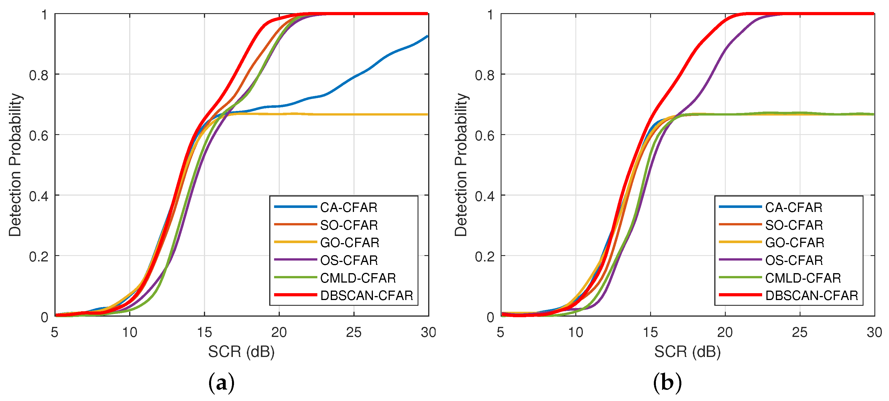
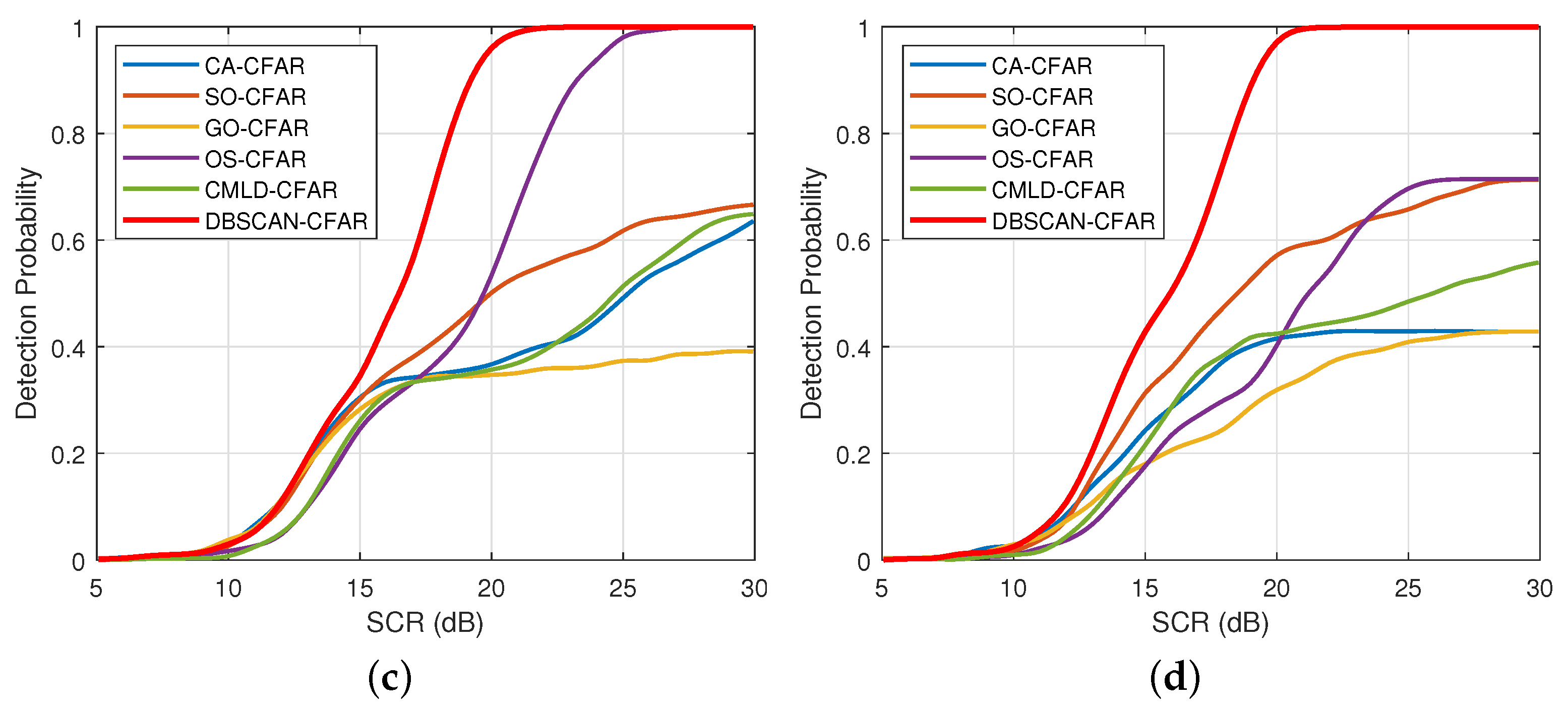
4.2. Impact of Interference Target Number

In multiple-target scenarios, we assume the primary target is located in the CUT to be processed, whereas the interference targets lie in different reference cells simultaneously. The existence of interference targets may cause evident target masking effect, which can seriously reduce the detection probability of the CFAR processor. Therefore, this subsection aims to investigate the tolerance of the number of interference targets for different CFAR processors, including the CA, SO, GO, OS, CMLD, and DBSCAN-CFAR.

Considering a background of K-distributed sea clutter, the number of range units is set to 500 and the shape parameter is estimated as $v_{est}=2.020$ by the proposed ANN model. One or more interference targets with the type of Swerling II are densely embedded in the clutter background to evaluate the detection performance of each processor. The interfering-to-clutter ratio (ICR) of the interference targets are considered with the same power of the main target. It is assumed that the sizes of reference cells and guard cells are $N=64$ and $M=4$ respectively. Specifically, set the parameters $k=60$ for OS-CFAR, $r=1$ for CMLD-CFAR, and $Eps=2$ and $MinPts=4$ for DBSCAN-CFAR as discussed in Section 3. Moreover, supposing the desired false alarm probability is $P_{fa}={10}^{-4}$, the corresponding threshold factor of the DBSCAN-CFAR processor can be acquired from the curve in Figure 8 with $\alpha =19.7$. To achieve the specified false alarm probability, each considered CFAR processor is applied through $1\times {10}^6$ Monte Carlo simulations for each SCR. After completing the all testing situations, the detection results of each processor are counted and compared.

Figure 10 depicts the detection probability $P_d$ versus the SCR in decibels from 5 to 30 dB. The numbers of interference targets in each subgraph are $m=1,2,4$, and 5 respectively, representing four typical multiple-target scenarios. As shown in Figure 10a, most of the processors SO, OS, CMLD, and DBSCAN-CFAR exhibit competitive detection performance due to only one interference target in the reference window. When the SCR is greater than 18.5 dB, the detection probability can reach 0.8 or higher. Since CA-CFAR does not consider the influence of interference targets when estimating the clutter background level, it may cause a missed alarm to the primary target and decline the detection performance. Although its detection probability can also reach more than 0.8, it increases the loss of about 6.5 dB compared with the aforementioned processors. Owing to the severe effect of target masking, GO-CFAR suffers the worst detection performance. Despite the SCR being greater than 16 dB, its detection probability is always maintained at 0.65 and no longer improved with the increasing SCR.

For the Figure 10b, when the number of interference targets is increased to $m=2$, OS-CFAR and DBSCAN-CFAR remain the favorable detection performance. However, CMLD-CFAR decreases significantly with a large drop in comparison of that in Figure 10a. The reason is that the number of interference values removed by the parameter $r=1$ is less than the number of interference targets. Similar to CA-CFAR, SO-CFAR, and GO-CFAR processors, the detection probability of CMLD-CFAR is truncated at 0.66 arbitrarily.

Referring to the Figure 10c, DBSCAN-CFAR still exhibits the optimal detection performance even the number of interference targets is $m=4$. Although the detection performance of OS-CFAR declines, it is superior to other processors except for DBSCAN-CFAR. As shown in Figure 10d, when the number of interference targets continues to increase to 5, the detection probability of OS-CFAR falls down from 1 to 0.71 at 30 dB because the number of interference targets exceeds the value of $N-k=4$. Nevertheless, the proposed processor can suppress the mutual target masking by yielding an outstanding and stable detection probability.

It can be stated from the results that, the detection performance of OS-CFAR and CMLD-CFAR in multiple-target scenarios is sensitive to their parameters r and k, which usually depend on the a priori information about the number and distribution of targets. In comparison, since the proposed DBSCAN-CFAR detector can self-adaptively eliminate the interference targets in the reference window as outliers by the DBSCAN clustering algorithm, the detection performance is almost unaffected by the increasing number of interference targets, even without prior information. From the above analysis, the proposed processor presents its advantages in tolerating multiple interference targets than others effectively.

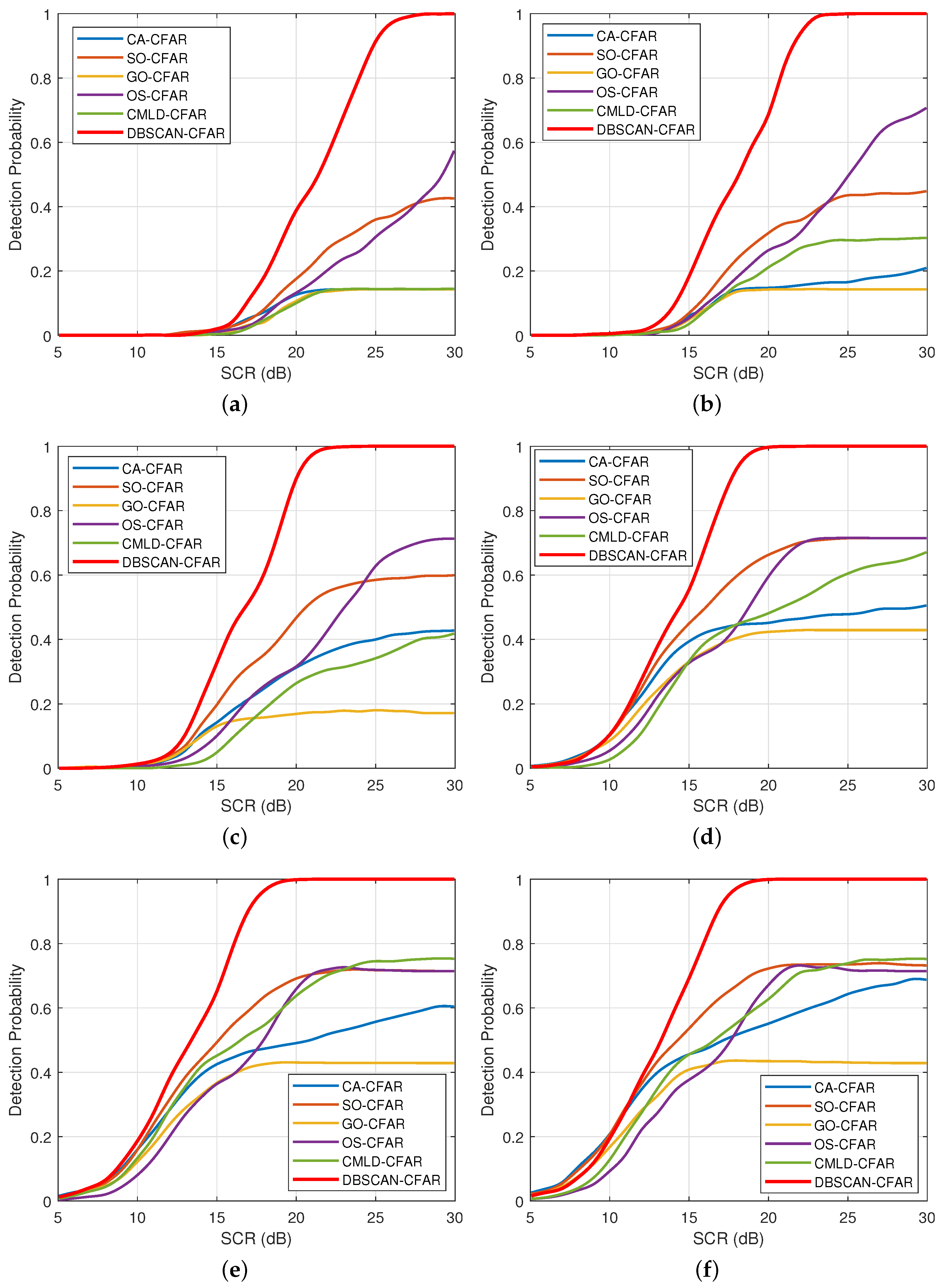
4.3. Impact of Various Shape Parameter

The purpose of the current subsection is to discuss the detection performance of CFAR processors with a fixed false alarm probability and varying shape parameters. Following the simulation settings in the previous subsection, assume that $P_{fa}={10}^{-4},N=64,M=4$, and the number of interference targets is $m=5$. In addition, the shape parameters are estimated to $v_{est}=0.201,0.502,1.023,6.027,10.109$, and 20.121 based on different sea clutter backgrounds, respectively. After that, the Monte Carlo simulations are described, which assessed the detection performance for all processors considered.

In Figure 11, the examples of clustering results by DBSCAN-CFAR are illustrated with one reference window at the SCR value of 15 dB. If paying attention to Figure 11c–f, it can be observed that the DBSCAN-CFAR processor can accurately separate the five interference targets from the background clutter as outliers. The reason lies in the fact that, there are no obvious sea spikes in the background clutter when the shape parameter is larger than 1, so that the outliers in each clustering result only contain the interference targets. However, as shown in Figure 11a,b with the shape parameters less than 1, sea spikes start to appear in the clustering of outliers except for the interference targets. The reduction in shape parameters increases the probability of the occurrence of sea spikes, which will affect the accuracy of estimating the background level, so that needs to be excluded.

Moreover, it should be noted that the color markers in Figure 11 represent the distribution of the amplitude of each clutter sample point, which is composed of the real part and the imaginary part of the complex radar echo, rather than the coordinate positions of sample points in the clutter sequence. Therefore, for two outliers that are far apart in the graph, their positions in the clutter sequence may be adjacent and may cause the target masking effect. Thanks to the insensitivity of the DBSCAN algorithm to the input order of the pending data, it was employed to eliminate outliers in the reference window, including interference targets and sea spikes, and to reduce the adverse effects on the estimation of background level.

Figure 12 presents the curves of detection probability against SCR with various shape parameters. It is intuitive that the detection probability of DBSCAN-CFAR is far superior to the remaining processors at the same multi-target scenarios. Additionally, comparing the curves of DBSCAN-CFAR in each subfigure, it can be seen that the detection performance is weakened as the shape parameter decreases from Figure 12a–f. Specifically, to achieve a detection probability of 0.8, the required SCR values for DBSCAN-CFAR at $v_{est}=20.121$, 1.023, and 0.201 are 15.75 dB, 19.25 dB, and 24 dB, respectively. The reason is that with the decrease of shape parameters, more sea spikes appear in the clutter background, which makes the processor require a higher SCR to reach the specified false alarm probability and detection probability.

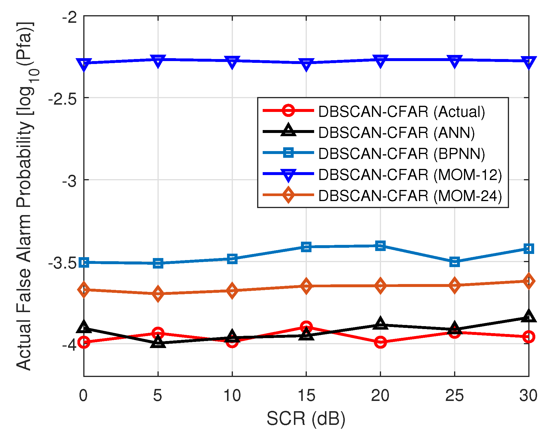
4.4. Impact of False Alarm Probability

In order to further verify the robustness of the proposed CFAR processors, the effects of different false alarm probabilities were investigated and compared with other processors. The simulation conditions in the Section 4.3 were continued, except for the estimated shape parameter of background clutter and the false alarm probability. These two items were configured as $v_{est}=0.302$ and $P_{fa}={10}^{-2},{10}^{-3},{10}^{-4}$, and ${10}^{-5}$.

Through Monte Carlo trials, the detection performance under different false alarm probabilities is plotted in Figure 13. As expected, the detection probability of DBSCAN-CFAR tends to increase gradually with the increasing SCR from 5 to 30 dB in each simulation case. For the curves of the DBSCAN-CFAR processor in subfigures, it is clearly that when the false alarm probability is reduced from ${10}^{-2}$ to ${10}^{-5}$, the overall detection performance is degraded visibly. In particular, when SCR = 20 dB, the detection probability of DBSCAN-CFAR at $P_{fa}={10}^{-2}$ is as high as 0.99, and 0.82 at $P_{fa}={10}^{-3}$, 0.51 at $P_{fa}={10}^{-4}$, and 0.35 at $P_{fa}={10}^{-5}$, respectively. However, even if the probability of false alarms changes, DBSCAN-CFAR still retains the optimal detection performance compared to the traditional processors, comprising CA, SO, GO, OS, and CMLD-CFAR. Analysis on these simulation results proves the superiority and stability of the proposed DBSCAN-CFAR detector under different false alarm probabilities.

4.5. Analysis of Time Elapsed

This subsection examines the execution speed of each processor in the working process, which is measured by the elapsed time covering the shape parameter estimation step and CFAR detection step. Based on the parameter configurations in Section 4.4, $1\times {10}^5$ Monte Carlo trials were performed to evaluate the average elapsed time.

Table 4. Comparisons of elapsed time for CFAR processors with various parameter estimation methods.

Processor	Runtime (ms)
	ANN	BPNN	MOM-12	MOM-24
CA-CFAR	81.1	80.6	47.8	55.8
SO-CFAR	79.3	78.8	46.0	54.0
GO-CFAR	78.4	77.9	45.1	53.1
OS-CFAR	79.6	79.1	46.3	54.3
CMLD-CFAR	81.7	81.2	48.4	56.4
DBSCAN-CFAR	325.1	324.6	291.8	299.8

enumerates the results of the detectors considered based on different parameter estimation methods, i.e., ANN, BPNN, MOM-12, and MOM-24. As shown, for a fixed parameter estimation method, such as ANN, the five processors of CA, SO, GO, OS, and CMLD-CFAR are basically in the same order of magnitude, approximately 80 milliseconds. However, DBSCAN-CFAR takes more computational time, up to 325.1 milliseconds, which is mainly spent on clustering operations for eliminating outliers in the reference window. Referring to the impact of different parameter estimation methods on the running time, we fixed our attention on the proposed DBSCAN-CFAR processor. For the ANN-based and BPNN-based DBSCAN-CFAR processors, their time overheads are comparable, at about 325 milliseconds. A similar outcome also resulted for the MOM-12 and MOM-24 approaches—295 milliseconds. In comparison, the NN-based DBSCAN-CFAR processors consumed more 30 milliseconds than the MOM-based ones. That is because using the NN-based methods for parameter estimation requires extracting the histogram features of the input radar clutter for adapting the trained network model. As a result, it can be revealed that the superiority of DBSCAN-CFAR with detection performance for multiple-target scenarios is at the expense of elapsed time. Moreover, noting that the offline training of the ANN model is accomplished in the design stage, it does not affect the real-time performance of DBSCAN-CFAR for estimating the shape parameters and detecting targets online.

5. Conclusions

In this paper, a machine learning based DBSCAN-CFAR processor is proposed to minify the deviation of the background level estimation in multiple-target scenarios for K-distributed sea clutter. At first, the shape parameter of the unknown background clutter was evaluated by various methods of the trained four-layer ANN model, BPNN, MOM-12, and MOM-24. With the estimated shape parameter, the corresponding threshold factor was derived for the specified false alarm probability. Subsequently, the clustering algorithm of DBSCAN was employed to eliminate the outliers in the reference window, including both interference targets and sea spikes. After that, the clutter background level was calculated exactly with the samples in the remaining reference cells. Finally, potential target detection can be achieved by comparing the CUT and the detection threshold, which is determined by the product of threshold factor and clutter background level. Compared with BPNN, MOM-12, and MOM-24, the ANN-based shape parameter estimation method yields a more accurate result for enabling the detector to control the actual false alarm probability at the desired level. Meanwhile, due to the distinctive clustering abilities, the ANN-based DBSCAN-CFAR processor can adaptively accommodate multiple interference targets in the reference window without prior knowledge of the number and distribution. Through extensive simulations, the superiority and robustness of the proposal are clearly demonstrated by outperforming the conventional processors of CA, SO, GO, OS, and CMLD-CFAR in scenarios with different target numbers, shape parameters, and false alarm probabilities. The cost is that DBSCAN-CFAR suffers from more computational burden and elapsed time than other processors. This paper promotes the organic integration of ANN and DBSCAN in the machine learning field with the traditional CFAR detection technologies to a certain extent. In the future, an extension of this work could be to optimize the clustering procedure for the proposed DBSCAN-CFAR processor theoretically and experimentally.

References

1. Greco, M.; Bordoni, F.; Gini, F. X-band sea-clutter nonstationarity: Influence of long waves. IEEE J. Ocean. Eng. 2004, 29, 269–283. [Google Scholar] [CrossRef]
2. Angelliaume, S.; Rosenberg, L.; Ritchie, M. Modeling the Amplitude Distribution of Radar Sea Clutter. Remote. Sens. 2019, 11, 319. [Google Scholar] [CrossRef] [Green Version]
3. Jakeman, E.; Pusey, P. A model for non-Rayleigh sea echo. IEEE Trans. Antennas Propag. 1976, 24, 806–814. [Google Scholar] [CrossRef]
4. Shi, S.; Shui, P. Optimum coherent detection in homogenous K-distributed clutter. IET Radar Sonar Navig. 2016, 10, 1477–1484. [Google Scholar] [CrossRef]
5. Lewinski, D. Nonstationary probabilistic target and clutter scattering models. IEEE Trans. Antennas Propag. 1983, 31, 490–498. [Google Scholar] [CrossRef]
6. Gandhi, P.P.; Kassam, S.A. Analysis of CFAR processors in nonhomogeneous background. IEEE Trans. Aerosp. Electron. Syst. 1988, 24, 427–445. [Google Scholar] [CrossRef]
7. Zhao, J.; Jiang, R.; Yang, H.; Wang, X.; Gao, H. Reconfigurable hardware architecture for Mean Level and log-t CFAR detectors in FPGA implementations. IEICE Electron. Express 2019, 16, 1–6. [Google Scholar] [CrossRef]
8. Weiss, M. Analysis of some modified cell-averaging CFAR processors in multiple-target situations. IEEE Trans. Aerosp. Electron. Syst. 1982, 18, 102–114. [Google Scholar] [CrossRef]
9. Hansen, V.G.; Sawyers, J.H. Detectability loss due to Greatest Of selection in a cell-averaging CFAR. IEEE Trans. Aerosp. Electron. Syst. 1980, 16, 115–118. [Google Scholar] [CrossRef]
10. Trunk, G.V. Range resolution of targets using automatic detectors. IEEE Trans. Aerosp. Electron. Syst. 1978, 14, 750–755. [Google Scholar] [CrossRef]
11. Rohling, H. Radar CFAR thresholding in clutter and multiple target situations. IEEE Trans. Aerosp. Electron. Syst. 1983, 19, 608–621. [Google Scholar] [CrossRef]
12. Rickard, J.T.; Dillard, G.M. Adaptive detection algorithms for multiple-target situations. IEEE Trans. Aerosp. Electron. Syst. 1977, 13, 338–343. [Google Scholar] [CrossRef]
13. Smith, M.E.; Varshney, P.K. Intelligent CFAR processor based on data variability. IEEE Trans. Aerosp. Electron. Syst. 2000, 36, 837–847. [Google Scholar] [CrossRef]
14. Ivković, D.; Andrić, M.; Zrnić, B.; Okiljević, P.; Kozić, N. CATM-CFAR detector in the receiver of the software defined radar. Sci. Tech. Rev. 2014, 64, 27–38. [Google Scholar]
15. Tao, D.; Anfinsen, S.N.; Brekke, C. Robust CFAR detector based on truncated statistics in multiple-target situations. IEEE Trans. Geosci. Remote. Sens. 2015, 54, 117–134. [Google Scholar] [CrossRef]
16. Zhou, W.; Xie, J.; Li, G.; Du, Y. Robust CFAR detector with weighted amplitude iteration in nonhomogeneous sea clutter. IEEE Trans. Aerosp. Electron. Syst. 2017, 53, 1520–1535. [Google Scholar] [CrossRef]
17. Domingos, P.M. A few useful things to know about machine learning. Commun. ACM 2012, 55, 78–87. [Google Scholar] [CrossRef] [Green Version]
18. Saxena, A.; Prasad, M.; Gupta, A.; Bharill, N.; Patel, O.P.; Tiwari, A.; Er, M.J.; Ding, W.; Lin, C. A review of clustering techniques and developments. Neurocomputing 2017, 267, 664–681. [Google Scholar] [CrossRef] [Green Version]
19. He, K.; Zhang, X.; Ren, S.; Sun, J. Deep residual learning for image recognition. In Proceedings of the IEEE Conference on Computer Vision and Pattern Recognition (CVPR), Las Vegas, NV, USA, 27–30 June 2016; IEEE: Las Vegas, NV, USA, 2016; pp. 770–778. [Google Scholar]
20. Peng, S.; Jiang, H.; Wang, H.; Alwageed, H.; Yu, Z.; Sebdani, M.M.; Yao, Y.D. Modulation classification based on signal constellation diagrams and deep learning. IEEE Trans. Neural Networks Learn. Syst. 2018, 30, 718–727. [Google Scholar] [CrossRef]
21. Jiang, R.; Wang, X.; Cao, S.; Zhao, J.; Li, X. Deep Neural Networks for Channel Estimation in Underwater Acoustic OFDM Systems. IEEE Access 2019, 7, 23579–23594. [Google Scholar] [CrossRef]
22. Fernández, J.R.M.; Vidal, J.D.B. Fast selection of the sea clutter preferential distribution with neural networks. Eng. Appl. Artif. Intell. 2018, 70, 123–129. [Google Scholar] [CrossRef]
23. Schwegmann, C.P.; Kleynhans, W.; Salmon, B.P.; Mdakane, L.W.; Meyer, R.G. Very deep learning for ship discrimination in synthetic aperture radar imagery. In Proceedings of the IEEE International Geoscience and Remote Sensing Symposium (IGARSS), Beijing, China, 10–15 July 2016; IEEE: Beijing, China, 2016; pp. 104–107. [Google Scholar]
24. Akhtar, J.; Olsen, K.E. A neural network target detector with partial CA-CFAR supervised training. In Proceedings of the International Conference on Radar (RADAR), Brisbane, Australia, 27–31 August 2018; IEEE: Brisbane, Australia, 2018; pp. 1–6. [Google Scholar]
25. Fernández, J.R.M.; Vidal, J.D.B.; Ferry, N.C. A neural network approach to Weibull distributed sea clutter parameter’s estimation. Intel. Artif. 2015, 18, 3–13. [Google Scholar] [CrossRef]
26. Fernández, J.R.M.; Vidal, J.D.B. Improved shape parameter estimation in Pareto distributed clutter with neural networks. Int. J. Interact. Multimed. Artif. Intell. 2016, 4, 7–11. [Google Scholar] [CrossRef] [Green Version]
27. Machado, J.F.; Vidal, J.D.B. Improved shape parameter estimation in K clutter with neural networks and deep learning. Int. J. Interact. Multimed. Artif. Intell. 2016, 3, 96–103. [Google Scholar]
28. Fernández, J.R.M.; Delgado, B.G.; Gil, A.M. A neural network approach to the recognition of the K distribution shape parameter associated with sea clutter. Rev. Ing. 2017, 27, 14–24. [Google Scholar]
29. Shen, J.; Hao, X.; Liang, Z.; Liu, Y.; Wang, W.; Shao, L. Real-time superpixel segmentation by DBSCAN clustering algorithm. IEEE Trans. Image Process. 2016, 25, 5933–5942. [Google Scholar] [CrossRef] [Green Version]
30. Hou, J.; Gao, H.; Li, X. DSets-DBSCAN: a parameter-free clustering algorithm. IEEE Trans. Image Process. 2016, 25, 3182–3193. [Google Scholar] [CrossRef]
31. Bryant, A.; Cios, K. RNN-DBSCAN: A density-based clustering algorithm using reverse nearest neighbor density estimates. IEEE Trans. Knowl. Data Eng. 2018, 30, 1109–1121. [Google Scholar] [CrossRef]
32. Zhou, W.; Xie, J.; Xi, K.; Du, Y. Modified cell averaging CFAR detector based on Grubbs criterion in non-homogeneous background. IET Radar Sonar Navig. 2018, 13, 104–112. [Google Scholar] [CrossRef]
33. Shui, P.; Liu, M.; Xu, S. Shape-parameter-dependent coherent radar target detection in K-distributed clutter. IEEE Trans. Aerosp. Electron. Syst. 2016, 52, 451–465. [Google Scholar] [CrossRef]
34. Roberts, W.J.; Furui, S. Maximum likelihood estimation of K-distribution parameters via the expectation-maximization algorithm. IEEE Trans. Signal Process. 2000, 48, 3303–3306. [Google Scholar]
35. Balleri, A.; Nehorai, A.; Wang, J. Maximum likelihood estimation for compound-Gaussian clutter with inverse gamma texture. IEEE Trans. Aerosp. Electron. Syst. 2007, 43, 775–779. [Google Scholar] [CrossRef]
36. Bouhlel, N.; Méric, S. Maximum-likelihood parameter estimation of the product model for multilook polarimetric SAR data. IEEE Trans. Geosci. Remote. Sens. 2018, 57, 1596–1611. [Google Scholar] [CrossRef]
37. Iskander, D.R.; Zoubir, A.M. Estimation of the parameters of the K-distribution using higher order and fractional moments. IEEE Trans. Aerosp. Electron. Syst. 1999, 35, 1453–1457. [Google Scholar] [CrossRef]
38. Ward, K.; Tough, R.; Watts, S. Sea Clutter: Scattering, the K-Distribution and Radar Performance, 2nd ed.; The Institution of Engineering and Technology: London, UK, 2013. [Google Scholar]
39. Roussel, C.J.; Coatanhay, A.; Baussard, A. Estimation of the parameters of stochastic differential equations for sea clutter. IET Radar Sonar Navig. 2018, 13, 497–504. [Google Scholar] [CrossRef]
40. Ester, M.; Kriegel, H.P.; Sander, J.; Xu, X. A density-based algorithm for discovering clusters in large spatial databases with noise. In Proceedings of the International Conference on Knowledge Discovery and Data Mining, Portland, OR, USA, 2–4 August 1996; AAAI Press: Portland, OR, USA, 1996; pp. 226–231. [Google Scholar]
41. Tran, T.N.; Drab, K.; Daszykowski, M. Revised DBSCAN algorithm to cluster data with dense adjacent clusters. Chemom. Intell. Lab. Syst. 2013, 120, 92–96. [Google Scholar] [CrossRef]
42. Chen, X.; Liu, W.; Qiu, H.; Lai, J. APSCAN: A parameter free algorithm for clustering. Pattern Recognit. Lett. 2011, 32, 973–986. [Google Scholar] [CrossRef]
43. Lai, W.; Zhou, M.; Hu, F.; Bian, K.; Song, Q. A new DBSCAN parameters determination method based on improved MVO. IEEE Access 2019, 7, 104085–104095. [Google Scholar] [CrossRef]
44. Manning, C.; Raghavan, P.; Schutze, H. Introduction to Information Retrieval; Cambridge University Press: Cambridge, UK, 2009. [Google Scholar]
45. Raghavan, R. A method for estimating parameters of K-distributed clutter. IEEE Trans. Aerosp. Electron. Syst. 1991, 27, 238–246. [Google Scholar] [CrossRef]
46. Li, C.; Xie, T.; Liu, Q.; Cheng, G. Cryptanalyzing image encryption using chaotic logistic map. Nonlinear Dyn. 2014, 78, 1545–1551. [Google Scholar] [CrossRef] [Green Version]
47. Li, Y.; Wang, N.; Shi, J.; Hou, X.; Liu, J. Adaptive batch normalization for practical domain adaptation. Pattern Recognit. 2018, 80, 109–117. [Google Scholar] [CrossRef]
48. Karlik, B.; Olgac, A.V. Performance analysis of various activation functions in generalized MLP architectures of neural networks. Int. J. Artif. Intell. Expert Syst. 2011, 1, 111–122. [Google Scholar]
49. Nair, V.; Hinton, G.E. Rectified linear units improve restricted boltzmann machines. In Proceedings of the 27th International Conference on Machine Learning, Haifa, Israel, 21–24 June 2010; Omnipress: Haifa, Israel, 2010; pp. 807–814. [Google Scholar]
50. Maas, A.L.; Hannun, A.Y.; Ng, A.Y. Rectifier nonlinearities improve neural network acoustic models. In Proceedings of the 30th International Conference on Machine Learning, Atlanta, GA, USA, 16–21 June 2013; Omnipress: Atlanta, GA, USA, 2013; pp. 1–6. [Google Scholar]
51. Armstrong, B.; Griffiths, H. CFAR detection of fluctuating targets in spatially correlated K-distributed clutter. IEE Proc. F (Radar Signal Process.) 1991, 138, 139–152. [Google Scholar] [CrossRef]
Figure 1. Block diagram of traditional constant false alarm rate (CFAR) processors.
Symmetry 11 01482 g001
Figure 2. Different thresholds for multiple-target scenario in K-distributed sea clutter.
Symmetry 11 01482 g002
Figure 3. Graphical presentation of mathematical definitions in the density-based spatial clustering of applications with noise (DBSCAN) algorithm.
Symmetry 11 01482 g003
Figure 4. Block diagram of the proposed DBSCAN-CFAR processor.
Symmetry 11 01482 g004
Figure 5. Clustering quality of the DBSCAN algorithm with different E p s and M i n P t s .
Symmetry 11 01482 g005
Figure 6. Training data sets with different segmentation methods for the artificial neural network (ANN) model.
Symmetry 11 01482 g006
Figure 7. Training performance of the network models with different number of neurons and hidden layers.
Symmetry 11 01482 g007
Figure 8. Relationship between threshold factor α and shape parameter v for different false alarm rates ( N = 64 , M = 4 ).
Symmetry 11 01482 g008
Figure 9. Impact of parameter estimation accuracy on the actual false alarm probability ( P f a = 10 4 ).
Symmetry 11 01482 g009
Figure 10. A comparative analysis of detection probabilities with various numbers of interference targets in the reference window ( N = 64 , P f a = 10 4 , v e s t = 2.020 ). (a) m = 1 . (b) m = 2 . (c) m = 4 . (d) m = 5 .
Symmetry 11 01482 g010aSymmetry 11 01482 g010b
Figure 11. Comparisons of the clustering results with varying shape parameters for the DBSCAN-CFAR processor ( N = 64 , P f a = 10 4 , m = 5 , S C R = 15 dB). (a) v e s t = 0.201 . (b) v e s t = 0.502 . (c) v e s t = 1.023 . (d) v e s t = 6.027 . (e) v e s t = 10.109 . (f) v e s t = 20.121 .
Symmetry 11 01482 g011
Figure 12. Comparisons of detection probabilities with various shape parameters ( N = 64 , P f a = 10 4 , m = 5 ). (a) v e s t = 0.201 . (b) v e s t = 0.502 . (c) v e s t = 1.023 . (d) v e s t = 6.027 . (e) v e s t = 10.109 . (f) v e s t = 20.121 .
Symmetry 11 01482 g012
Figure 13. Comparisons of detection probabilities with different false alarm probabilities ( N = 64 , v e s t = 0.302 ). (a) P f a = 10 2 . (b) P f a = 10 3 . (c) P f a = 10 4 . (d) P f a = 10 5 .
Symmetry 11 01482 g013