Novel Fuzzy Clustering Methods for Test Case Prioritization in Software Projects

 , and
, and
Abstract
1. Introduction
2. Related Studies of Test Case Prioritization (TCP)
Model-Based Black-Box Techniques
- Clustering methods proposed in the literature are single-sided clustering, that is, clustering is done from the perspectives of test cases. This will cause potential information loss, as the interrelationship between test cases and faulty functions is ignored.
- The similarity measures used in literature do not concentrate on the distribution of the data (input), which affects the convergence process. Moreover, literature studies do not provide methods pertaining to accuracy and time separately, and this is an open challenge to address.
- Prioritization methods do not consider inter- and intra-clustering, which eventually causes loss of information.
- Finally, customization on constraints is not dominantly provided in TCP. This would restrict the convergence and cause inaccuracies.
- Challenge one is resolved by proposing a novel two-way clustering that clusters both test cases and faulty functions for better understanding the interrelationship among them.
- Challenge two is addressed by proposing a new similarity measure that utilizes the power of exponent measure and provides smoothening of data for effective convergence. Further, the distribution of the data is also taken into consideration, and dominancy measure is proposed along with similarity measure for properly managing accuracy time trade-off.
- The WASPAS method is extended for inter- and intra-clustering prioritization, which effectively prioritizes test cases.
- Finally, the programming model is put forward for better customization of parameters to obtain an optimal test case for the set of faulty functions.
3. Proposed Methodology
3.1. Proposed Fuzzy-Similarity Test Case Prioritization (TCP) Model (FSTPM)
| Algorithm 1: Pseudo code for fuzzy-similarity test case prioritization model (FSTPM) |
| Input: Given F = [Lij], for i = 1, 2, …, n and j = 1, 2, …, m are the linguistic relationship matrix between the set of n-test cases and m-faulty items. |
| Output: F1 = [aij], for i = 1, 2, …, n and j = 1, 2, …, m, with clustering partition between the set of test cases and faultiness. |
| 1. Using Gaussian membership function, convert the given F-linguistic relationship matrix into F1 = [bij] for i = 1, 2, …, n and j = 1, 2, …, m as fuzzy matrix |
| 2. To compute fuzzy 0–1 matrix F2 = [aij] for i = 1, 2, …, n and j = 1, 2, …, m from F1 by using the relation where |
| 3. for i = 1 to n do |
| { |
| for j = 1 to n do |
| { |
| i. to compute a, b, c and d values between the ith and jth row |
| ii. to compute the similarity between the test cases by using the relation |
| } |
| } |
| 4. using the similarity index Sij as obtained from step-3, to solve the following 0–1 programming: |
| where |
| subject to the constraints |
| 5. Apply steps 3 and 4 for faultiness and based on the yij, values, group/cluster the faultiness |
| 6. Based on the group of test cases and the faultiness, rearrange the rows and columns of F2, then we got the clustering. This will be the given input of an inter and intra ranking of clusters |
3.2. Dominancy Test Based Clustering for Test Case Prioritization (DTTCP)
| Algorithm 2: Pseudo code for dominancy test for test case prioritization (DTTCP) |
| Input: Given F = [Lij], for i = 1, 2, …, n and j = 1, 2, …, m are the linguistic relationship matrix between the set of n-test cases and m-faulty items. Output: F2 = [aij], for i = 1, 2, …, n and j = 1, 2, …, m, with clustering partition between the set of test cases and faultiness (or) Recommended to move to FSTPM with reduced F2 fuzzy 0–1 matrix
|
3.3. Discussion
3.4. An Inter and Intra Ranking of Clusters
- Step 1:
- Obtain k clusters each having an evaluation matrix of order m by n where m denotes the number of test cases, and n denotes the number of criteria.
- Step 2:
- The values in these matrices are linguistic. These are converted into fuzzy values by using Gaussian membership function.
- Step 3:
- Initially, the dominant cluster is estimated by using the weighted arithmetic method given in Equation (15). The weight of each test case is considered to be equal, and this helps the procedure to pay equal attention to each test case.where n is the number of criteria, is the weight of the criteria with , and and is the fuzzy value.
- Step 4:
- Using step 3, the weighted arithmetic value of each test case pertaining to a particular cluster is obtained. The average is calculated for each cluster, and these values are normalized to obtain the weight of the cluster. They are given by Equations (16) and (17):where p is the number of clusters taken for the study.
- Step 5:
- From step 4, the weight of each cluster is obtained, and using these values dominant cluster can be determined.
- Step 6:
- The matrix of order m by n is chosen from the dominant cluster, and the test cases are ranked using the WASPAS method. The formulations are given by Equations (18)–(20):where is the weighted sum method (WSM), is the weighted product method (WPM), is the final rank value is the weight of the jth criterion with and and is the strategy value with .
- Step 7:
- The value is obtained for each test case and the test case, which has the highest value is a highly preferred test case and so on.
4. Numerical Example
4.1. Illustration of Clustering of Test Cases


4.2. An illustrative Example for Inter and Intra Test Case Prioritization
5. A Real Case Study Analysis
6. Conclusions
Author Contributions
Funding
Acknowledgments
Conflicts of Interest
Appendix A

| Symbol | Description |
|---|---|
| F | Fuzzy linguistic matrix |
| F1 | Fuzzy matrix of F |
| F2 | Fuzzy 0–1 matrix |
| Lij | Linguistic relationship between the test case i and faulty item j |
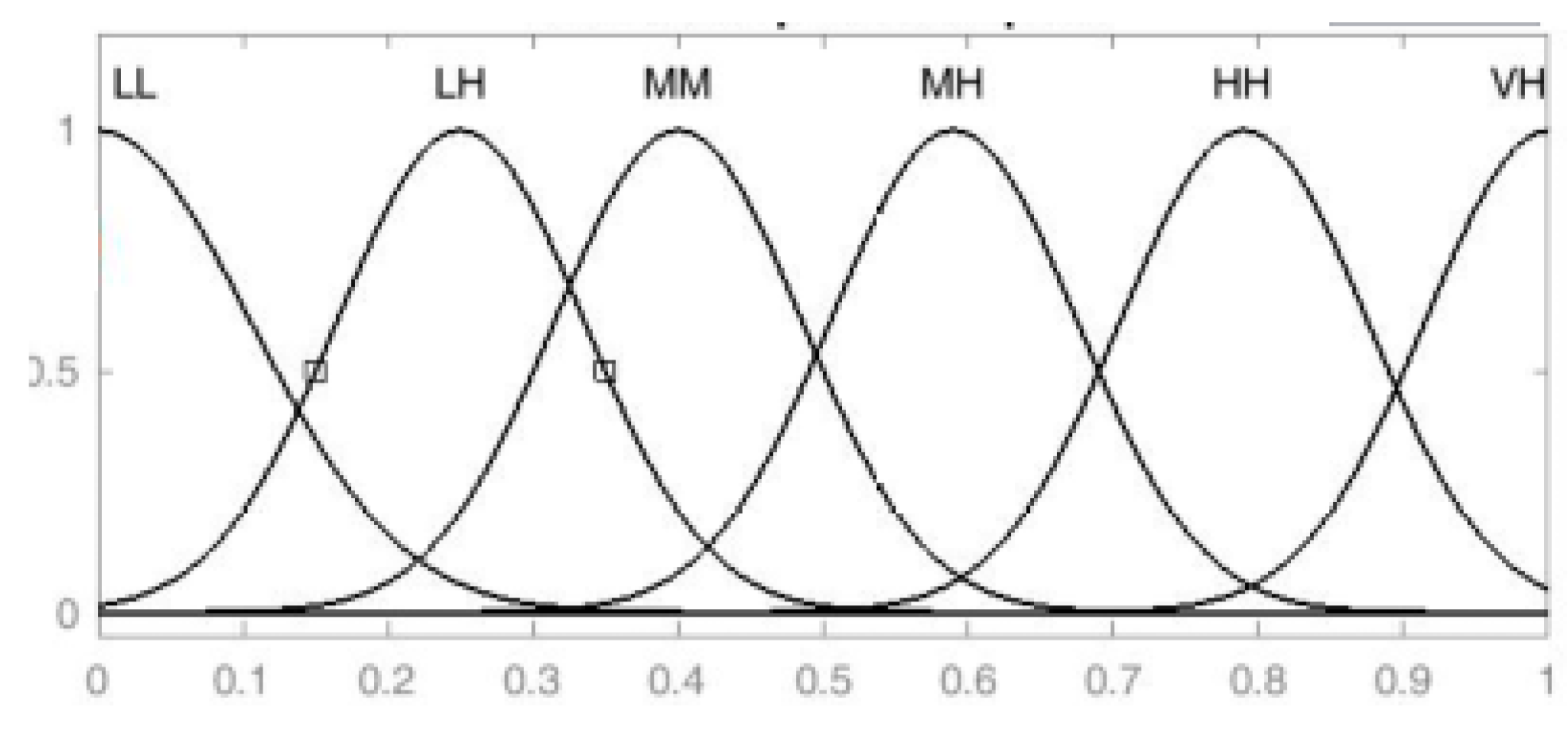
| LL | Low |
| LH | Low-high |
| MM | Medium |
| MH | Medium-high |
| HH | High |
| TCi | Test case i |
| fj | Faulty item j |
| aij | 1 if the faultiness j is in test case i; otherwise 0 |
| a | Faulty item is occurring in both the test cases i and j, while finding the similarity coefficient between ith and jth test cases |
| b | Faulty item is occurring in the test case i but not j |
| c | Faulty item is occurring in the test case j but not i |
| d | Faulty item is not occurring in both of the test cases i and j |
| N | Total number of test cases |
| M | Total number of faultiness available in the test cases |
| Gc | Number of permissible groups |
| ρ | Maximum number of permissible test cases |
| υ | Threshold value |
| Sij | Similarity between test cases i and j / faultiness j and j |
| yij | Decision variables used during test cases grouping |
| xij | Decision variables used during faultiness grouping |
| Ta | Test case a |
| Ti | ith faults |
| Wi | Weight criteria i |
| μij | Fuzzy value between ith and jth criterion |
| Weighted arithmetic value | |
| Average weighted arithmetic | |
| Normalized weighted arithmetic | |
| Weighted sum method | |
| Weighted product method | |
| Final rank | |
| Strategy value |
References
- Wang, R.; Jiang, S.; Chen, D.; Zhang, Y. Empirical Study of the effects of different similarity measures on test case prioritization. Math. Probl. Eng. 2016. [Google Scholar] [CrossRef]
- Srikanth, H.; Banerjee, S. Improving test efficiency through system test prioritization. J. Syst. Softw. 2012, 85, 1176–1187. [Google Scholar] [CrossRef]
- Yu, Y.T.; Lau, M.F. Fault-based test suite prioritization for specification-based testing. Inf. Softw. Technol. 2012, 54, 179–202. [Google Scholar] [CrossRef]
- Rothermel, G.; Untch, R.H.; Chu, C.; Harrold, M.J. Prioritizing Test Cases for Regression Testing. IEEE Trans. Softw. Eng. 2001, 27. [Google Scholar] [CrossRef]
- Huang, Y.-C.; Peng, K.-L.; Huang, C.-Y. A history-based cost-cognizant test case prioritization technique in regression testing. J. Syst. Softw. 2012, 85, 626–637. [Google Scholar] [CrossRef]
- Chittimalli, P.K.; Harrold, M.J. Recomputing coverage information to assist regression testing. IEEE Trans. Softw. Eng. 2009, 35, 452–469. [Google Scholar] [CrossRef]
- Yoo, S.; Harman, M. Regression testing minimisation, selection and prioritisation: A survey. Test Verif. Reliab. 2007, 22, 1–7. [Google Scholar]
- Jeffrey, D.; Gupta, N. Improving fault detection capability by selectively retaining test cases during test suite reduction. IEEE Trans. Softw. Eng. 2007, 33, 108–123. [Google Scholar] [CrossRef]
- Elbaum, S.; Kallakuri, P.; Malishevsky, A.G.; Rothermel, G.; Kanduri, S. Understanding the effects of changes on the cost-effectiveness of regression testingtechniques. J. Softw. Test. Verif. Reliab. 2003, 12, 65–83. [Google Scholar] [CrossRef]
- Rothermel, G.; Untch, R.H.; Chu, C.C.; Harrold, M.J. Test case prioritization: An empirical study. In Proceedings of the IEEE International Conference on Software Maintenance, (ICSM 99), Oxford, UK, 30 August–3 September 1999; pp. 179–188. [Google Scholar]
- Elbaum, S.; Malishevsky, A.G.; Rothermel, G. Test case prioritization: A family of empirical studies. IEEE Trans. Softw. Eng. 2002, 28, 159–182. [Google Scholar] [CrossRef]
- Khalilian, A.; Azgomi, M.A.; Fazlalizadeh, Y. An improved method for test case prioritization by incorporating historical test case data. Sci. Comput. Program. 2012, 78, 93–116. [Google Scholar] [CrossRef]
- Huang, C.-Y.; Chang, J.-R.; Chang, Y.H. Design and analysis of GUI test-case prioritization using weight-based methods. J. Syst. Softw. 2010, 83, 646–659. [Google Scholar] [CrossRef]
- Chen, J.; Zhu, L.; Chen, T.; Towey, D.; Kuo, F.-C.; Huang, R.; Guo, Y. Test Case Prioritization for Object-Oriented Software: An adaptive random sequence approach based on clustering. J. Syst. Softw. 2018, 135, 107–125. [Google Scholar] [CrossRef]
- Muhammad, K.; Isa, M.A.; Jawawi, D.N.A.; Tumeng, R. Test case prioritization approaches in regression testing: A systematic literature review. Inf. Softw. Technol. 2018, 93, 74–93. [Google Scholar]
- Singh, Y. Systematic literature review on regression test prioritization techniques. Informatica 2012, 36, 379–408. [Google Scholar]
- Catal, C.; Mishra, D. Test case prioritization: A systematic mapping study. Softw. Qual. J. 2012, 21, 445–478. [Google Scholar] [CrossRef]
- Kumar, A.; Singh, K. A Literature Survey on Test Case Prioritization. Compusoft 2014, 3, 793. [Google Scholar] [CrossRef]
- Kiran, P.; Chandraprakash, K. A literature survey on TCP-test case prioritization using the RT-regression techniques. Glob. J. Res. Eng. 2015. Available online: https://engineeringresearch.org/index.php/GJRE/article/view/1312 (accessed on 11 October 2019).
- Jeffrey, D.; Gupta, N. Experiments with test case prioritization using relevant slices. J. Syst. Softw. Sci. Direct. 2007, 196–221. [Google Scholar] [CrossRef]
- Lijun, M.; Chan, W.K.; Tse, T.H.; Robert, G. Merkel. XML-manipulating test case prioritization for XML-manipulating services. J. Syst. Softw. 2011, 84, 603–619. [Google Scholar] [CrossRef]
- Krishnamoorthi, R.; Sahaaya Arul Mary, S.A. Factor oriented requirement coverage based system test case prioritization of new and regression test cases. Inf. Softw. Technol. 2009, 51, 799–808. [Google Scholar] [CrossRef]
- Thomas, S.W.; Hemmati, H.; Hassan, A.E.; Blostein, D. Static test case prioritization using topic models. Empir. Softw. Eng. 2012. [Google Scholar] [CrossRef]
- Do, H.; Rothermel, G. On the use of mutation faults in empirical assessments of test case prioritization techniques. IEEE Trans. Softw. Eng. 2006, 32. [Google Scholar] [CrossRef]
- Zhai, K.; Bo, J.; Chan, W.K. Prioritizing Test Cases for Regression Testing of Location-Based Services: Metrics, Techniques, and Case Study. IEEE Trans. Serv. Comput. 2014, 7, 54–67. [Google Scholar] [CrossRef]
- Haidry, S.; Miller, T. Using Dependency Structures for Prioritization of Functional Test Suites. IEEE Trans. Softw. Eng. 2013, 39, 258–275. [Google Scholar] [CrossRef]
- Srikanth, H.; Hettiarachchi, C.; Do, H. Requirements based test prioritization using risk factors: An Industrial Study. Inf. Softw. Technol. 2016, 69, 71–83. [Google Scholar] [CrossRef]
- Hettiarachchi, C.; Do, H.; Choi, B. Risk-based test case prioritization using a fuzzy expert system. Inf. Softw. Technol. 2016, 69, 1–15. [Google Scholar] [CrossRef]
- Huang, R.; Chen, J.; Towey, D.; Chan, A.T.S.; Lu, Y. Aggregate-strength interaction test suite prioritization. J. Syst. Softw. 2015, 99, 36–51. [Google Scholar] [CrossRef]
- Jiang, B.; Chan, W.K. Input-based adaptive randomized test case prioritization: A local beams approach. J. Syst. Softw. 2015, 105, 91–106. [Google Scholar] [CrossRef]
- Ledru, Y.; Petrenko, A.; Boroday, S.; Mandran, N. Prioritizing test cases with string distances. Autom. Softw. Eng. 2012, 19, 65–95. [Google Scholar] [CrossRef]
- Zhang, C.; Chen, Z.; Zhao, Z.; Yan, S.; Zhang, J.; Xu, B. An improved regression test selection technique by clustering execution profiles. In Proceedings of the 10th International Conference on Quality Software (QSIC’10), Washington, DC, USA, 14–15 July 2010; pp. 171–179. [Google Scholar] [CrossRef]
- Jiang, B.; Zhang, Z.; Chan, W.; Tse, T. Adaptive random test case prioritization. In Proceedings of the 24th International Conference on Automated Software Engineering (ASE’09), Auckland, New Zealand, 16–20 November 2009; pp. 233–244. [Google Scholar] [CrossRef]
- Breno, M.; Bertolino, A. Scope-aided test prioritization, selection and minimization for software reuse. J. Syst. Softw. 2017, 131, 528–549. [Google Scholar]
- Kim, J.M.; Porter, A. A History-based Test Prioritization Technique for Regression Testing in Resource Constrained Environments. In Proceedings of the 24th International Conference on Software Engineering, Orlando, FL, USA, 19–25 May 2002; pp. 119–129. [Google Scholar] [CrossRef]
- Fang, C.; Chen, Z.; Wu, K.; Zhao, Z. Similarity based test case prioritization using ordered sequence of program entities. Softw. Qual. J. 2014, 22, 335–361. [Google Scholar] [CrossRef]
- Noor, T.B.; Hemmati, H. A similarity-based approach for test case prioritization using historical failure data. In Proceedings of the 2015 IEEE 26th International Symposium on Software Reliability Engineering (ISSRE), Gaithersbury, MD, USA, 2–5 November 2015. [Google Scholar]
- Gokce, N.; Belli, F.; Eminli, M.; Dincer, B.T. Model-based test case prioritization using cluster analysis: A soft-computing approach. Turk. J. Electr. Eng. Comput. Sci. 2015, 23, 623–640. [Google Scholar] [CrossRef]
- Li, Z.; Harman, M.; Hierons, R.M. Search algorithms for regression test case prioritization. IEEE Trans. Softw. Eng. 2007, 33, 225–237. [Google Scholar] [CrossRef]
- Elberzhager, F.; Rosbach, A.; Munch, J.; Eschbach, R. Reducing test effort: A systematic mapping study on existing approaches. Inf. Softw. Technol. 2012, 54, 1092–1106. [Google Scholar] [CrossRef]
- Elbaum, S.; Rothermel, G.; Kanduri, S.; Malishevsky, A.G. Selecting a Cost-Effective Test Case Prioritization Technique. Softw. Qual. J. 2004, 12, 185–210. [Google Scholar] [CrossRef]
- Do, H.; Mirarab, S.; Tahvildari, L.; Rothermel, G. The effects of Time Constraints on Test Case Prioritization: A Series of Controlled Experiments. IEEE Trans. Softw. Eng. 2010, 36, 593–617. [Google Scholar] [CrossRef]
- Shrivathsan, A.D.; Ravichandran, K.S. Meliorate test efficiency: A survey. World Appl. Sci. J. 2014, 133–139. [Google Scholar] [CrossRef]
- Mohammed, A.R.; Mohammed, A.H.; Mohammed, S.S. Prioritizing Dissimilar Test Cases in Regression Testing using Historical Failure Data. Int. J. Comput. Appl. 2018, 180. [Google Scholar] [CrossRef]
- Chaurasia, G.; Agarwal, S. A Hybrid Approach of Clustering and Time-aware based Novel Test Case Prioritization Technique. Int. J. Database Theory Appl. 2016, 9, 23–44. [Google Scholar] [CrossRef]
- Mohammed, J.A.; Do, H. Test Case Prioritization using Requirements-Based Clustering. In Proceedings of the 2013 IEEE Sixth International Conference on Software Testing, Verification, and Validation, Luxembourg, 18–22 March 2013; pp. 312–321. [Google Scholar] [CrossRef]


| Alternative | Sum | Product | Rank |
|---|---|---|---|
| A1 | 0.84 | 0.834 | 0.83 |
| A2 | 0.526 | 0 | 0.26 |
| A3 | 0.716 | 0.706 | 0.711 |
| A4 | 0.55 | 0 | 0.275 |
| Alternative | Sum | Product | Rank |
|---|---|---|---|
| A1 | 0.813 | 0.81 | 0.81 |
| A2 | 0.8 | 0.79 | 0.7959 |
| A3 | 0.786 | 0.77 | 0.781 |
| Alternative | Sum | Product | Rank |
|---|---|---|---|
| A1 | 0.42 | 0 | 0.21 |
| A2 | 0.776 | 0.7749 | 0.7758 |
| Objects | Language | Req. | Versions | Size (KLoC) | Classes | # Faulty Versions | Fault Types | Bug Type | Bug Description |
|---|---|---|---|---|---|---|---|---|---|
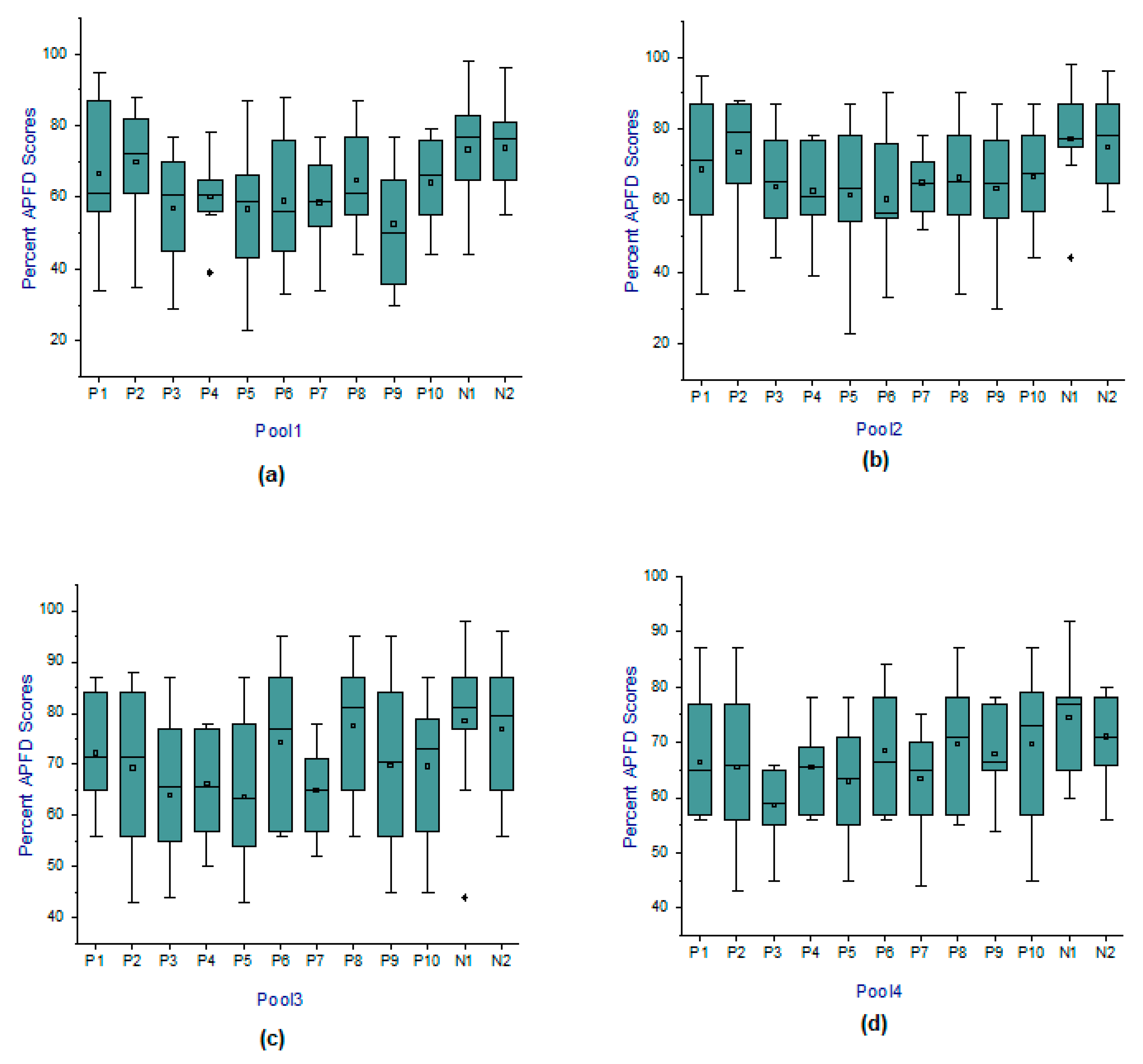
| Pool 1 | Java | 19 | 2 | 3.62 | 28 | 36 | Real | Race | Thread execution order and execution speed problem |
| Pool 2 | Java | 59 | 2 | 18.66 | 88 | 114 | Real | Deadlock | Resource allocation contention problem |
| Pool 3 | Java | 123 | 3 | 38.09 | 124 | 136 | Real | Deadlock | Resource allocation contention problem |
| Pool 4 | Java | 84 | 4 | 20.43 | 94 | 112 | Real | Deadlock | Resource allocation contention problem |
| Proposed Methods | Pool 1 No. of Clusters | Pool 2 No. of Clusters | Pool 3 No. of Clusters | Pool 4 No. of Clusters | ||||||||
|---|---|---|---|---|---|---|---|---|---|---|---|---|
| 3 | 6 | 9 | 3 | 6 | 9 | 3 | 6 | 9 | 3 | 6 | 9 | |
| N1 | 73.21 | 72.56 | 69.23 | 73.48 | 78.36 | 75.86 | 74.16 | 77.12 | 73.57 | 73.31 | 74.67 | 71.78 |
| N2 | 71.97 | 71.64 | 70.05 | 74.51 | 76.43 | 74.09 | 74.82 | 76.07 | 75.66 | 66.85 | 70.96 | 68.32 |
© 2019 by the authors. Licensee MDPI, Basel, Switzerland. This article is an open access article distributed under the terms and conditions of the Creative Commons Attribution (CC BY) license (http://creativecommons.org/licenses/by/4.0/).
Share and Cite
Shrivathsan, A.D.; Ravichandran, K.S.; Krishankumar, R.; Sangeetha, V.; Kar, S.; Ziemba, P.; Jankowski, J. Novel Fuzzy Clustering Methods for Test Case Prioritization in Software Projects. Symmetry 2019, 11, 1400. https://doi.org/10.3390/sym11111400
Shrivathsan AD, Ravichandran KS, Krishankumar R, Sangeetha V, Kar S, Ziemba P, Jankowski J. Novel Fuzzy Clustering Methods for Test Case Prioritization in Software Projects. Symmetry. 2019; 11(11):1400. https://doi.org/10.3390/sym11111400
Chicago/Turabian StyleShrivathsan, A. D., K. S. Ravichandran, R. Krishankumar, V. Sangeetha, Samarjit Kar, Pawel Ziemba, and Jaroslaw Jankowski. 2019. "Novel Fuzzy Clustering Methods for Test Case Prioritization in Software Projects" Symmetry 11, no. 11: 1400. https://doi.org/10.3390/sym11111400
APA StyleShrivathsan, A. D., Ravichandran, K. S., Krishankumar, R., Sangeetha, V., Kar, S., Ziemba, P., & Jankowski, J. (2019). Novel Fuzzy Clustering Methods for Test Case Prioritization in Software Projects. Symmetry, 11(11), 1400. https://doi.org/10.3390/sym11111400