1. Introduction
Mathematical models based on random differential and difference equations consider input parameters as random variables or stochastic processes [
1,
2,
3]. The aim of this kind of models is to capture the uncertainty often met in the analysis of complex phenomena. This randomness comes from errors in measurements or estimations, a lack of information, or ignorance of the phenomenon under analysis, etc. In particular, these are typical features in dealing with the study of epidemiological models, where input data, such as the initial proportion of infected individuals, the rates of contagious and recovery caused by an infectious disease, etc., are not deterministically known. In such a situation, it is more realistic to model all this initial information via random variables or stochastic processes rather than by using deterministic constants or functions, respectively. These facts have motivated the development of powerful mathematical techniques capable to model and quantify uncertainty in dealing with epidemiological problems to better understand and describe the dynamics of a disease.
Given the response stochastic process, the primary goal of Uncertainty Quantification consists in understanding the main probabilistic features of the model outputs, by computing their statistical moments (mainly the mean and the variance), confidence intervals, etc. [
4]. The most well-known method to approach this problem is Monte Carlo simulation [
5]. It is easy to implement and effective, although computationally expensive. An alternative is based on generalized polynomial chaos (gPC) expansions and the stochastic Galerkin projection technique [
6,
7,
8,
9,
10,
11,
12,
13,
14,
15,
16], which usually converges at an algebraic/exponential rate (exponential convergence) [
6,
17,
18].
Apart from computing the mean and the variance, a major goal in dealing with stochastic models is to calculate the set of (first) probability density functions of the solution process at each time instant [
1] (p. 35). By means of the probability density function, all the statistical moments and confidence intervals corresponding to the solution process can be determined [
1] (Chapters 2–3). When dealing with stochastic problems with a closed-form solution, the Random Variable Transformation (RVT) technique has been widely used to calculate the density function of the solution, see [
19,
20,
21] in the setting of random differential equations, [
21,
22,
23,
24,
25,
26] in the context of random partial differential equations, and [
27] for random difference equations. When no explicit form of the solution is available or it is given via infinite analytic expressions (such as random power series, random eigenfunctions expansions, etc.), one usually constructs a sequence of approximating processes, whose exact density functions (computed via the RVT technique) form a sequence of approximating density functions that converge rapidly. This methodology has been carried out via numerical methods [
28], Karhunen-Loève expansions [
29,
30], or random power series [
29,
31], and it has supposed an improvement compared with Monte Carlo simulations and Kernel density estimations in terms of rate of convergence and accuracy.
In the recent contribution [
9], RVT and gPC techniques have been successfully combined to study random differential equations. That study focused on the computation of the mean and the variance of the solution stochastic process for random differential equations. In the present paper, we combine both techniques to go further and to compute reliable approximations to the probability density function of stochastic models. Furthermore, we point out that the proposed method possesses rapid convergence and is able to reach its goal even in the case that no closed-form solution to the stochastic problem is available. This is a distinctive feature of our approach since, as it has been previously indicated, the application of the RVT technique to determine the probability density function of stochastic models usually requires knowing a closed-form expression of the solution, see for instance [
19,
20,
21,
22,
23,
24,
25,
26]. All these features of our approach will be illustrated through several epidemiological models. At this point it is important to underscore that in the context of epidemiological modeling, knowledge of the probability density function is crucial, since from it, apart from computing predictions (via the mean) and confidence intervals (via the mean and the standard deviation), one can also compute the probability that the proportion of infected individuals lies in a certain interval of interest for health authorities [
19,
32,
33] (prevention and control of plagues, identify seasonal patterns of infection, etc.).
Hereinafter, we will work with stochastic models with only one random input parameter. The reason for this restriction is that there is a version of the RVT technique for non-injective transformation mappings on with many applications in general, but not on , . The RVT method will allow us to compute the exact density function of the Galerkin projections (which are polynomials, usually non-injective), and by taking limits we will approximate the density function of the response process. Since the Galerkin projections converge at algebraic/exponential rate to the solution process, it is expected to have rapid convergence of the sequence of approximating density functions.
From a modeling standpoint, the variability of each parameter (input) produces a variability in the results (output) of the model. However, the effects of the variabilities of the parameters are of different magnitude and can be estimated by using a sensitivity analysis method such as gPC-based Sobol’s indices [
12,
34,
35,
36]. These indices explain the influence of each random parameter on the response process, by performing a variance-based sensitivity analysis. The variance of the output is a sum of contributions of each input variable and combinations of them. Indeed, the variance of the output is the squared-sum of the Galerkin coefficients, so the contribution of the main effect of a parameter is the normalized squared-sum of the coefficients corresponding to basis polynomial functions evaluated only at the aforesaid parameter. By computing Sobol’s indices, it is assumed that the parameter that leads to a larger variance of the output has the largest effect on the model prediction. If one is dealing with epidemic models, the parameter with highest gPC-based Sobol’s index is the most important to address and control the epidemic, and the other parameters may be taken to be deterministic. Therefore the fact of introducing randomness into only one input parameter may be justified.
The structure of the paper is the following. In
Section 2, we will specify the type of stochastic problems under study, we will show the necessary basics of gPC expansions and the RVT technique, and we will combine both methods to approximate the probability density function of the solution stochastic process. In
Section 3, we will illustrate the theoretical development with several particular examples of continuous and discrete stochastic models in an epidemiological and social setting. Finally,
Section 4 will draw conclusions.
2. Method
We consider an initial value differential equation problem with one degree of uncertainty:
or
where
is an interval,
,
F is a deterministic function, and
is the random input parameter, which can be the initial condition (case (
1)), or can appear in the differential equation expression (case (
2), with the initial condition
being deterministic). The random variable
is assumed to be absolutely continuous (we denote its density function by
) with centered absolute moments of any order. At this point, it is important to point out that the largest part of random variables that are used in practice, specially in epidemiological modeling, such as Beta, Gaussian, Gamma, Uniform, Triangular, etc., satisfy these hypotheses. In this setting, we are assuming an underlying complete probability space
, where
is the sample space consisting of outcomes
,
is the
-algebra of events and
is the probability measure.
The solution
to (
1) or (
2) is a stochastic process. We will assume that such a solution exists and is unique, in some stochastic sense (sample path sense, mean square sense, etc., see [
1,
2]). Our goal is to compute the probability density function of
,
, at each time instant
. The density function allows performing uncertainty quantification for
, since all the statistical moments and confidence intervals can be derived from it [
1] (Chapters 2–3).
Other alternative stochastic systems to (
1) and (
2) are possible as well: random partial differential equations, random difference equations, etc., with one degree of uncertainty. For such stochastic systems, the techniques exposed here work analogously.
2.1. gPC Expansions
Given the random input parameter
, consider its associated canonical basis
, for each degree
. By using a Gram-Schmidt procedure, we orthonormalize this basis in the Hilbert space of random variables with well-defined variance,
, where the inner product is defined as
for
, being
the expectation operator with respect to the probability measure
. Let
be the orthonormal basis of
,
, where
. For example, if
, then
is the set of Hermite polynomials; if
, then
is formed by Legendre polynomials, etc. [
6,
7]. Notice that, with this approach, we are not restricted to distributions from the Askey scheme [
6] (Chapter 3), as already remarked in [
8,
9]. This point has great interest in practice, since most of the random variables constructed to model real phenomena do not fit the standard distributions, and therefore we are enlarging the applicability of the classical gPC method.
If
Z is a random variable in
written as a function of
,
, then the gPC expansion of
Z is
, where the sum is considered in
and the Fourier coefficients
are given by
. Actually, to ensure that
, we need that the moment problem is uniquely solvable for
, see [
37] (Th. 3.3). This condition is not so restrictive, as any random variable with finite moment-generating function in a neighborhood of the origin has a uniquely solvable moment problem [
37] (Th. 3.4).
If we take the solution stochastic process
, then we may formally write
in
, where
. The Fourier coefficients
cannot be explicitly computed, as
is unknown. We use the stochastic Galerkin projection technique [
6,
7,
8,
9]: We seek a solution of the form
, i.e., we impose
The deterministic functions
are calculated in two steps: first, we multiply the previous equation by
, and we take the expectation operator and use the orthonormality of
:
and secondly, we solve a deterministic system of differential equations via standard numerical techniques. Formally,
in
. Some general results justify this assertion, see [
17,
18]. Moreover, algebraic/exponential convergence usually holds (spectral convergence).
The stochastic Galerkin projection technique and gPC expansions have been profusely used in the literature for uncertainty quantification, see for example [
10,
11,
12,
13,
14,
15,
16].
We will show how to compute exactly the probability density function of , which will be used as an approximation for .
2.2. RVT Technique
The RVT technique has been successfully applied to study significant random ordinary differential equations [
19,
20,
21,
28], random partial differential equations [
21,
22,
23,
24,
25,
26,
30] and random recursive equations [
27], that appear in different areas such as Epidemiology, Physics, Engineering, etc. In this paper, we will use the following version of the RVT technique:
Theorem 1 ([
38] (p. 115)).
Let X be an absolutely continuous random variable with density and with support contained in an open set . Let be such that and is injective and with non-vanishing derivative. Then the random variable is absolutely continuous, with density function given by Although there is a version of this theorem for , , its applicability in our context will be reduced to . For example, when working with transformation mappings g given by polynomials (this will be the case of the Galerkin projections), in dimension one we can find the regions by equating the derivative to 0; however, polynomials on , , is a different matter, as the regions may be impossible to find or even not exist. This fact motivates that in this first step of our research we consider the case , which has specific interest.
2.3. Combining gPC and RVT Technique to Approximate the Density Function
Fixed
and
, the Galerkin projection
is an explicit transformation of the random variable
, let us call it
. Since
is a polynomial, by solving numerically
we can determine the sets
where
g is strictly monotone and find
. At each
, by finding numerically the unique root
such that
, we compute the inverse of
,
. By the RVT technique,
Since
has been computed numerically for each
, we do not have
explicitly. We compute
as
instead. Thus,
Notice that the RVT technique has permitted us to obtain the exact expression for the probability density function of the Galerkin projection . This exact expression is a distinctive feature of the RVT technique comparing with other stochastic methods (for example, gPC expansions plus Monte Carlo simulations for the Galerkin projections).
Since
in
at algebraic/exponential rate, we expect to have
with rapid convergence. This procedure works as a computational method to approximate
. To the best of our knowledge, there are no available theoretical results that guarantee that (
4) holds, but only mean square convergence of the Galerkin projections
, instead.
In principle, we know nothing about the type of convergence of the sequence to the true density . The numerical experiments that we will carry out in the forthcoming section, see Example 1 for instance, show that uniform convergence may not be expected, as might be discontinuous but continuous. Hence, in general, one may expect convergence of in some Lebesgue space.
Assume that is Cauchy in . By the completeness of the Lebesgue spaces, there is a function such that in , for each . Then the limit function is a density function for . Indeed, notice that is a density function, because almost everywhere and . Let be a stochastic process such that . We have that in law as , since . On the other hand, since in , in particular in law, as , we conclude that and are equal in distribution, therefore is absolutely continuous and . Thus, if the sequence is Cauchy, then the limit function must be .
In practice, we have to be careful with the order of truncation
p chosen, since if
p is too large, numerical errors may arise, see [
17,
18,
39,
40] (Section 4). This is a disadvantage of gPC expansions. There may be an order of truncation
such that, for any
, the results obtained make no sense, therefore the density function may not be computed as accurately as wanted. See the forthcoming Example 3.
3. Numerical Experiments
In this section, we deal with particular continuous and discrete stochastic models that play an important role in Epidemiology. By using the previous ideas, we will approximate the probability density function of the solution stochastic process to some epidemiological models at different time instants. In the field of Epidemiology, the computation of the probability density function is a primary goal, as the expected number or confidence intervals for infective (predictions), or any other information of interest for health authorities, can be derived from it.
The computations have been carried out in the software Mathematica
®, version 11.2 (Wolfram Research, Inc.: Champaign, IL, USA, 2017) [
41], installed on an Intel
® Core
TM i7 CPU 3.1 GHz. To compute the roots of
and
, the built-in function
NSolve has been utilized. The solution to deterministic systems of differential equations has been solved by means of the standard
NDSolve routine, with automatic method, step size, etc.
When dealing with real data, we will compute deterministic estimates for the model parameters with a least squares fitting procedure (
FindFit built-in function). Then we will introduce a small perturbation into one of the parameters (with mean value being the deterministic estimate calculated) and we will apply the methodology previously exposed. Introducing only a small amount of randomness into the model from deterministic estimates allows a more faithful representation of the time evolution of the population, see for example [
8] (Example 5), [
12,
13,
14,
42]. In this article, as we are interested in testing our methodology on approximating the density function of the model output, but not in estimating probability distributions for the input parameters, we do not deal with inverse parameter estimation, see, for example, references [
6] (pp. 95–99), [
43,
44], related with Bayesian inference and gPC expansions.
In the examples, we will see that it suffices to take a small order
p of basis to get accurate approximations of the probability density function. The optimal
p is that from which the subsequent probability density functions constructed for larger orders than
p are virtually the same. In previous contributions dealing with approximations of the mean and variance statistics in the setting of continuous and discrete epidemic models (SIS, SIR, etc. models), see [
10,
14], it was shown numerically that, although for
the approximations are not good, for
and
very similar results are produced.
In Example 1, the approximations of the probability density functions constructed by combining gPC expansions and the RVT technique will be compared with the exact density function. For Examples 2–4, we will compare our approximations against a Kernel density estimation from Monte Carlo simulations sampled from the stochastic problem directly, with the built-in function
SmoothKernelDistribution of Mathematica
®. We will check that Kernel density estimations do not approximate well when the sought density function is not smooth (see the documentation on the built-in function
SmoothKernelDistribution, or the theoretical reference [
45]), while our method substantiated on the RVT technique is certainly able to identify discontinuities and peaks, i.e., the exact shape of the target density function. Moreover, gPC-based methods converge much faster than Monte Carlo simulations, even when there is only one random input coefficient, see the discussions from previous contributions [
6,
7,
8]. Indeed, Monte Carlo simulations converge relatively slow (for example, the mean value converges at rate
, where
m is the number of realizations), whereas gPC expansions converge at spectral rate.
When no explicit form of the solution is available, representations of it via infinite expansions (gPC expansions, random power series, Karhunen-Loève expansions, etc.) or discretizations from numerical methods are usually required. By truncating these infinite expansions or from the discretizations, one constructs a sequence of approximating processes, whose exact density functions (computed via the RVT technique) form a sequence of approximating density functions that converge rapidly [
28,
29,
30,
31]. In terms of rapidity and accuracy, this sort of approximations are preferable to Monte Carlo simulations and Kernel density estimations.
In Remark 1 from Example 4, we will show how gPC-based Sobol’s indices (see
Section 1) may be used to determine the parameter whose variability has the most important effects and therefore justify the fact of introducing uncertainty into one input parameter only, in the context of a social model for addictive behavior.
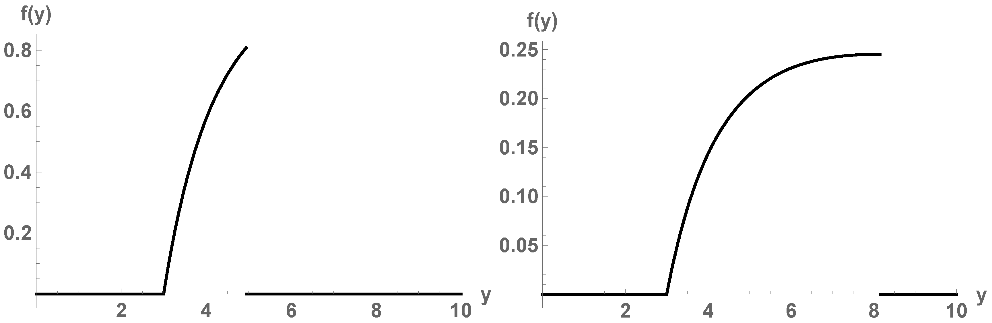
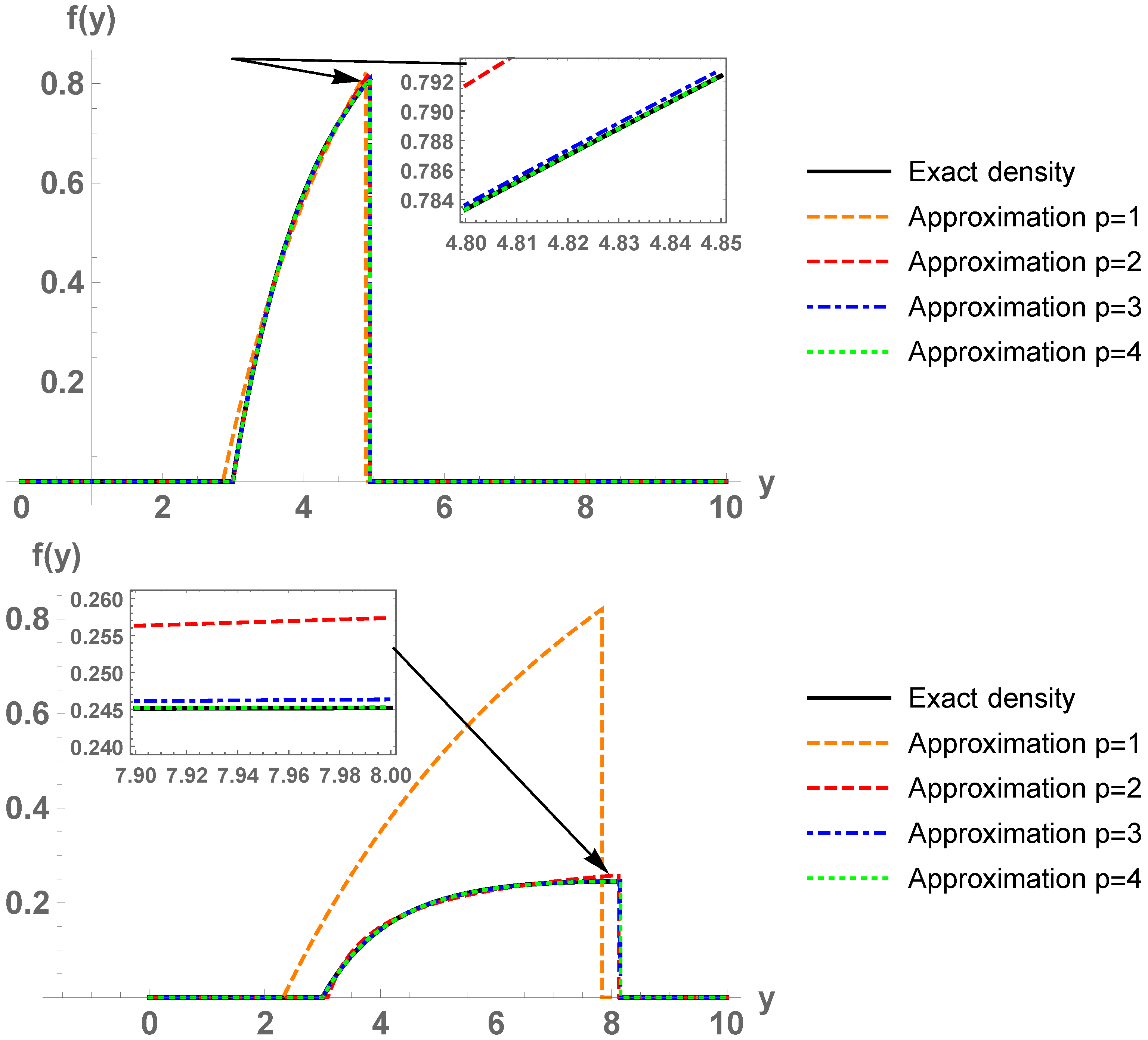
Example 1. In this example, we consider the simplest continuous epidemiological model to describe the growth of a population of bacteria with no limitation of resources and no antibiotics (predators). The model has demonstrated to be still useful to describe this population growth in presence of competitors during the initial stage. Proposed by Thomas Malthus in 1798 in his essay [46], this model is considered as the first law of population dynamics and is usually referred to as exponential or Malthusian model [47] (Chapter 1), [48]. With the aim of illustrating the main ideas exhibited in the previous section, next we deal with the following particular case of the Malthusian model which has been addressed in [6] (p. 69–70), [7] (p. 10):where . This initial value problem may correspond to a bacteria with initial population 3 million of individuals and whose relative instantaneous growth rate fluctuates randomly in the unit interval. For this stochastic model, the solution stochastic process is well-known: . By means of the RVT technique, the exact probability density function of can be calculated: Figure 1 plots for and . Let us test our methodology. We use our computational method to approximate the probability density function of at the times and . In Figure 2 we show the corresponding results. We observe that, as the order of basis p increases, the sequence of density functions of the Galerkin projections tends to . Based on observation of Figure 2, this convergence seems to hold in , , but not uniformly on , since seems continuous for . Table 1 shows the error for each order p: This integral has been calculated in Mathematica® with the standardNIntegrateroutine. Observe that the error decreases to 0 very fast (exponentially), although convergence deteriorates when time t increases.
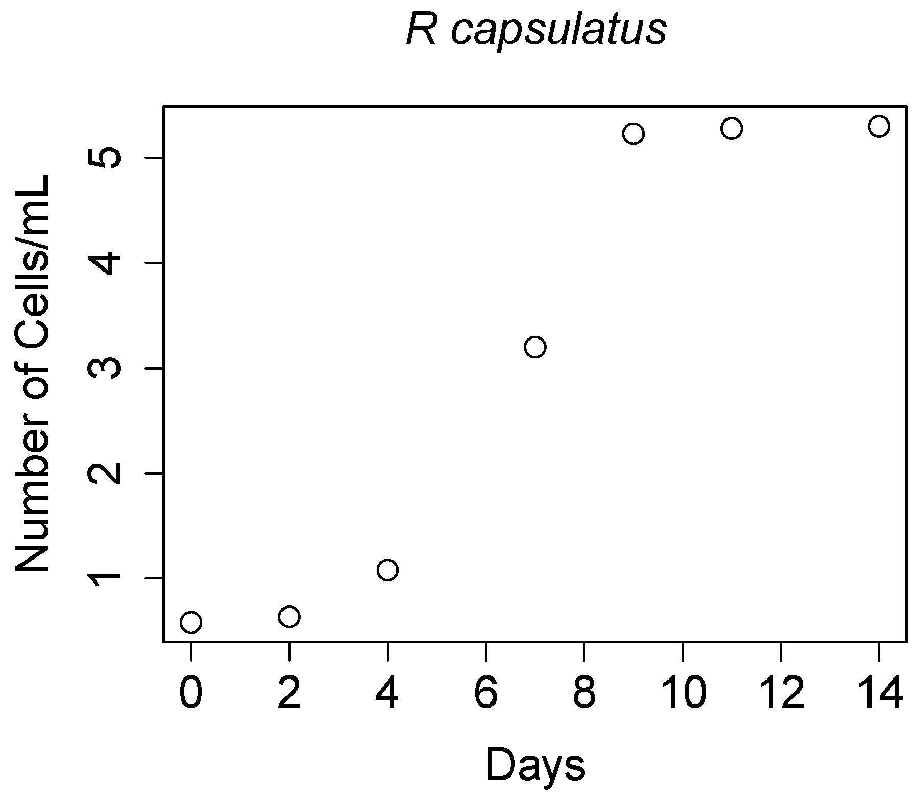
Example 2. In this example, we deal with a stochastic model applied to real laboratory data of bacteria growth [42]. We consider a species of bacteria from a laboratory experiment: Rhodobacter capsulatus (R. capsulatus). Direct cell counts were made every two or three days until a stationary phase was achieved. For more information regarding the experiment, we refer the reader to [42]. Table 2 shows the population sizes of R. capsulatus under infrared lightning conditions in different mediums. The number of cells/mL has been rescaled by dividing by . Figure 3 plots the cell counts from Table 2. In [42], the authors used the Malthusian model to describe the bacteria growth at the first 9 days (before the stationary phase), while a logistic equation model was applied up to day 14
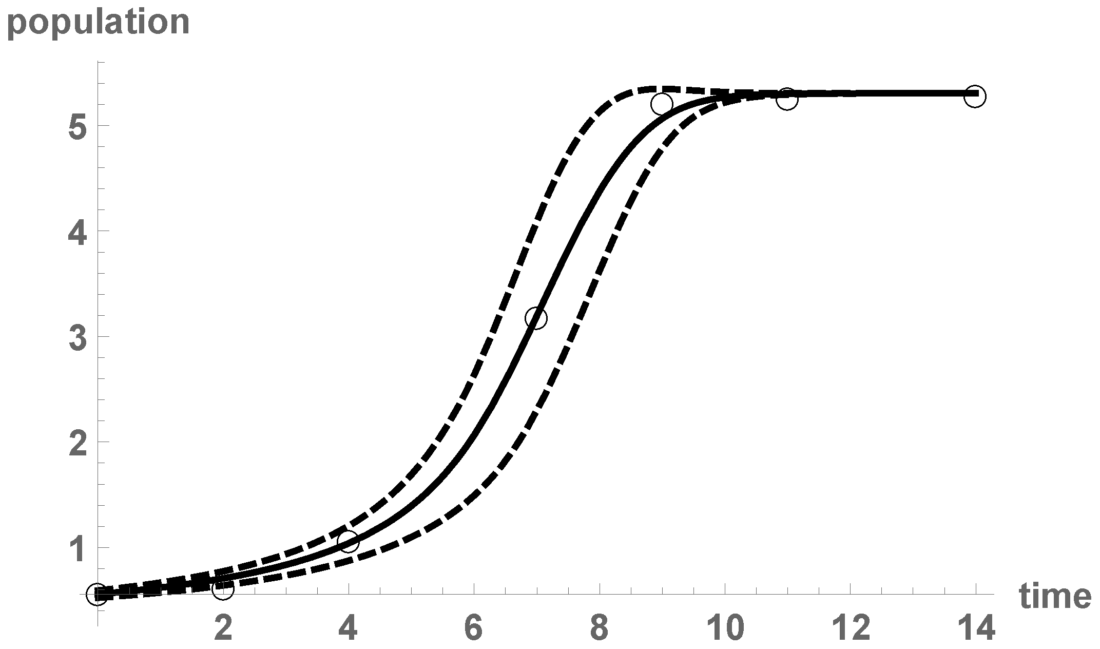
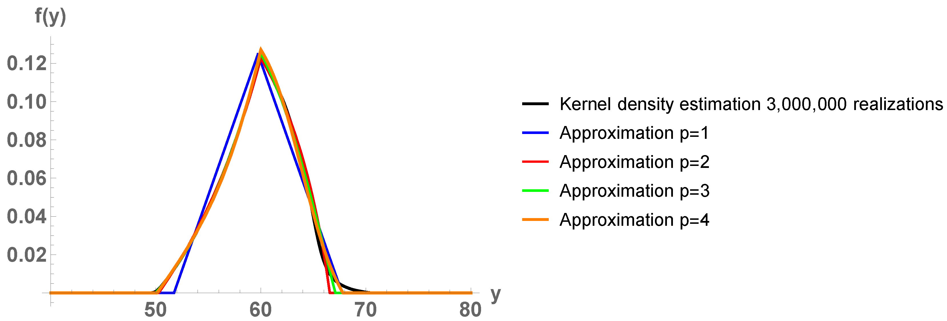
. In this example, we suppose that the growth rate is not proportional to the total number of individuals , but to the total number of interactions, , via a parameter r. Moreover, we take into account the competition for the limited resources with a carrying capacity (limit population under no death assumption), and also the beginning of the bacteria decline phase via a death parameter . The parameters r, K, and δ are assumed to be deterministic, while the initial condition ζ is taken as a random variable:This Equation (5) corresponds to the simplified Fitzhugh-Nagumo model [49] (p. 2). A least squares fitting gives the deterministic estimates , , , and , with a very small residual squared error (smaller than the exponential growth model and the logistic equation presented in [42]). To randomize the initial condition ζ, we consider a distribution centered at : . The introduction of randomness into the initial condition requires the search of suitable techniques to perform uncertainty quantification. Via gPC expansions and the stochastic Galerkin projection technique with order of basis (this is enough to achieve convergence), pointwise estimates via , and a confidence interval with the rule , can be constructed, see Figure 4. Observe that the actual data belong to the confidence interval and that the solid line reflects properly the growth of the bacteria population. Notice also that the confidence interval is wider in the middle of the growth phase, while smaller uncertainty seems to occur near the initial condition and the carrying capacity. By using our previous exposition on the combination of the RVT method and gPC expansions, we are even able to determine the probability density function of . In Figure 5, we plot the approximations for . The similarity of the approximating density functions shows that convergence has been achieved. Our results have been compared with a Kernel density estimation with the built-in functionSmoothKernelDistribution. The densities constructed via gPC expansions show that, possibly, the limit density function has two jump discontinuities, therefore the Kernel density estimation does not approximate well those discontinuities and draws tails. Table 3 shows consecutive errors for orders of truncation p and , : Notice that the error decreases to 0 very fast.
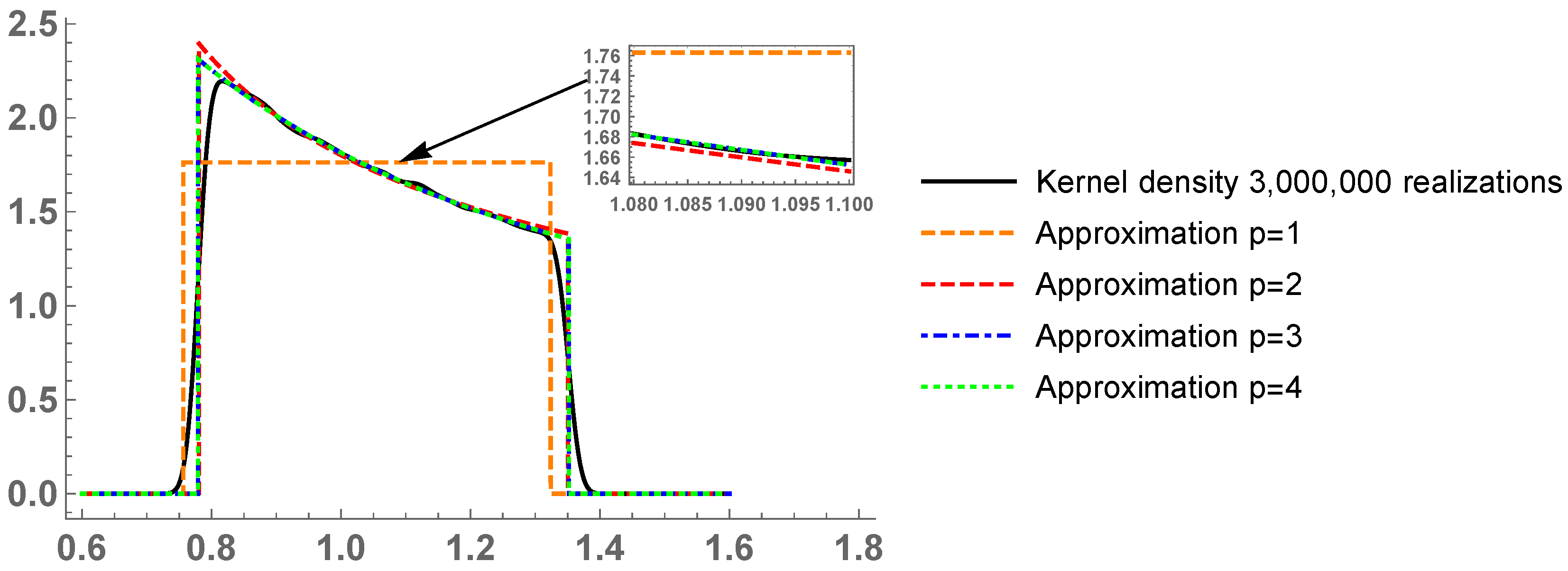
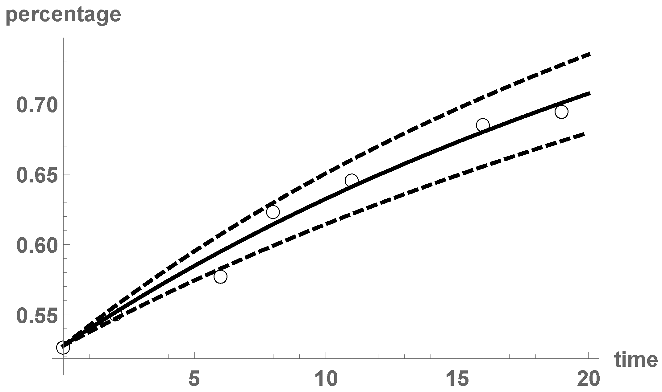
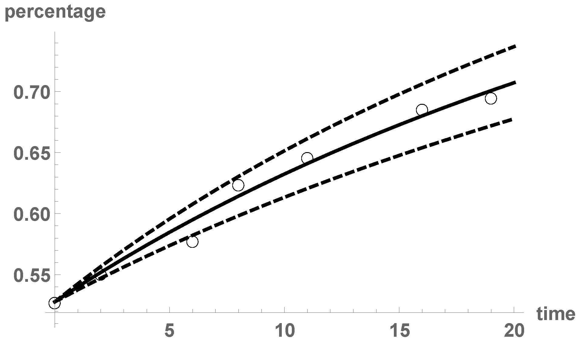
Example 3. We deal with uncertainty quantification for the following discrete stochastic system [18] (Section 4):where . In the epidemiological context, if and denote, respectively, the number of susceptible and infected individuals in a population of one hundred individuals at the period (e.g., months), the above discrete system describes the dynamics for the number of infected individuals over the time (in months). The parameter ξ can be interpreted as the contagious rate at which a susceptible becomes infected. More precisely, by considering that the product defining the right-hand side of the difference equation gives the number of encounters between susceptible individuals () and infected individuals (), then the parameter ξ can be interpreted as the probability that such encounters be successful (i.e., the disease spreading). Since the value of this probability depends upon complex factors such as immunity of each individual of the population, weather, etc., whose nature is unpredictable, it is more realistic to treat ξ as random variable instead of being a deterministic number. As previously indicated and for illustrative purposes only, we will assume that ξ lies in the interval according to a triangular distribution. As a consequence, at each time step m, the solution is a random variable. The Galerkin projection takes the form , where the deterministic coefficients satisfy a difference equation. The stochastic Galerkin projection technique has not been applied to discrete models with the same emphasis as with continuous models. In our recent contributions [14,18], the applications of gPC to discrete dynamical systems have been analyzed. For a large time m, the explicit expression of cannot be obtained or is too complex, so the application of the transformation method is inviable. Thus, one needs appropriate methods to perform uncertainty quantification for . We think that the combination of the RVT technique and gPC expansions is a good approach to try uncertainty quantification for . The computation of the probability density function of is a step beyond the numerical experiment performed in ([18], Section 4), as [18] only considered the approximation of the expectation and variance statistics. We approximate the probability density function at . In Figure 6, we show the results. From , catastrophic numerical errors invalidate the results. Thus, we are restricted to , and we cannot approximate the density function as accurately as desired. This illustrates the main drawback of our computational method. Our results have been compared with a Kernel density estimation with the built-in functionSmoothKernelDistribution. Notice that, since the sought density function seems not smooth (there may be three peaks because of the triangular form), the Kernel density estimation might not approximate well near the peaks. Example 4. In this example, we deal with a social model for the addictive behavior of smoking. We use the data from our recent contribution [14] (Table 1), with original source the National Spanish Health Survey [50]. In Table 4, we show the percentage of nonsmokers Spanish men aged over 16 years old during the period 1995–2014, denoted by , . As in [14], we use a discrete SIS model: SIS-type models are useful to describe the spread of diseases (smoking) whose infection does not confer immunity [32,48,51]. In the model formulation, a is the proportion of infective (smokers) that leave this compartment (people giving up tobacco), and b is the proportion of contacts between susceptible and infective (non-smokers and smokers) that give rise to a new infected individual (smoker). We are assuming homogeneous mixing, i.e., all individuals are equally likely to contact any other individual. We are also supposing a constant total population . Since our data reflects percentages, we take . From , we can get rid of the second equation and work with the first one: In our usual notation, . By using a least squares fitting procedure, the best deterministic estimates for a and b are and . We introduce randomness into a, with distribution . The infection parameter b is constant: .
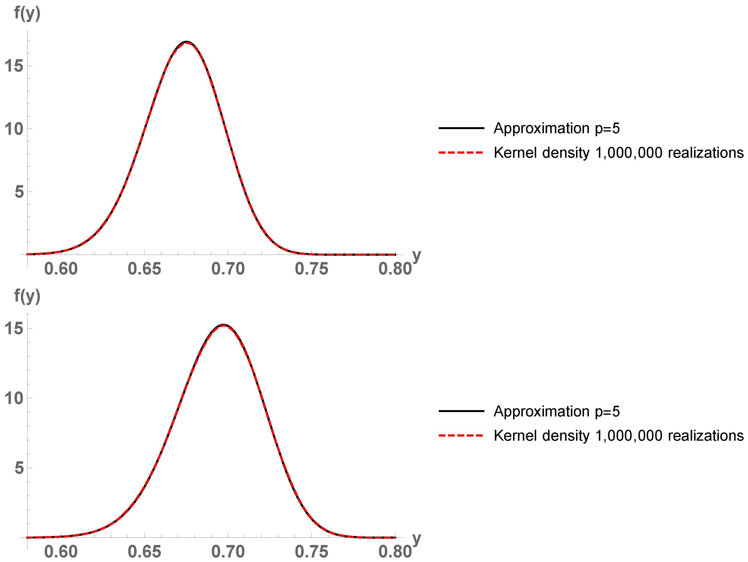
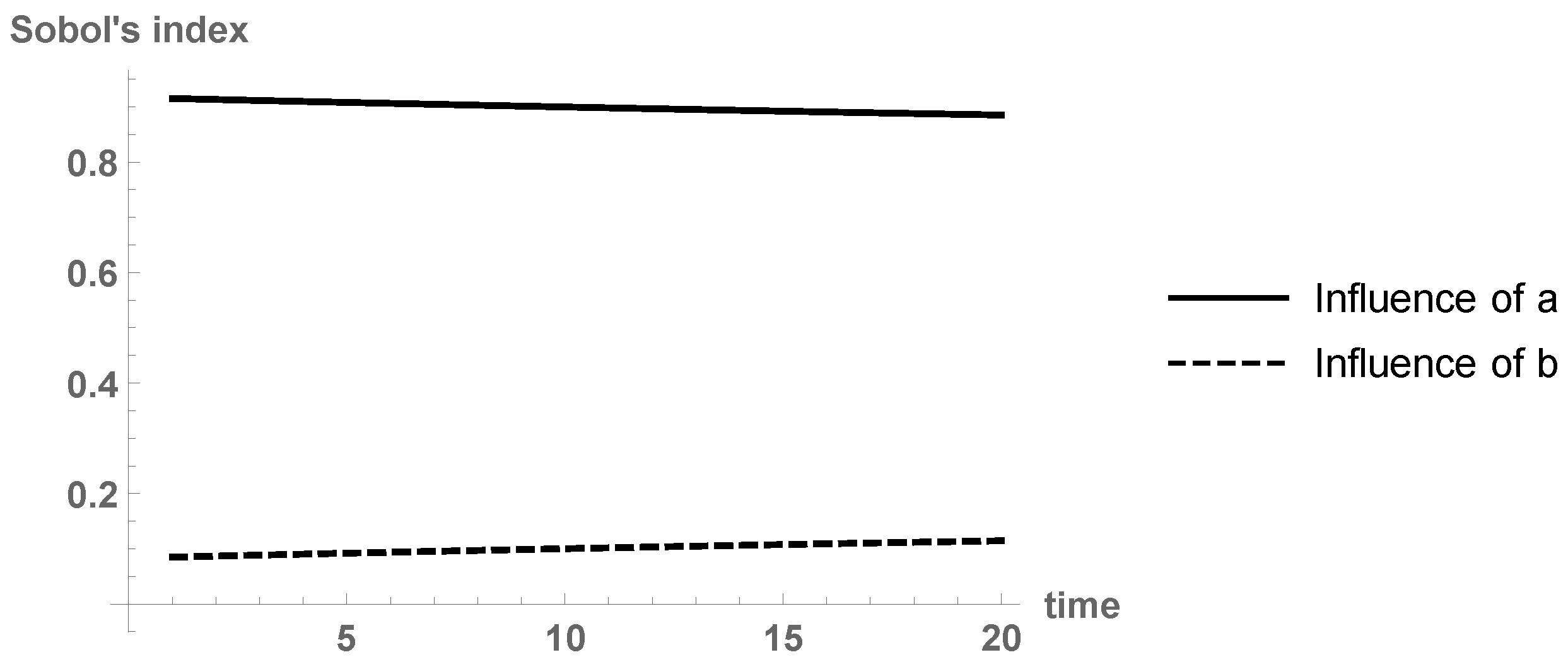
By using a gPC approach with , we approximate the expectation and variance of susceptible individuals . Figure 7 plots the results. We observe that the proposed SIS model captures the uncertainty of the smoking habit. By combining the RVT technique and gPC expansions, we can go a step further and compute the probability density function of at times and , see Figure 8. With orders of basis , the results agree with a Kernel density estimation with the built-in functionSmoothKernelDistribution. In this case, since the density function of seems smooth (with no peaks), the Kernel density estimation is correct. Remark 1. As we commented, by using a least squares fitting procedure, the best deterministic estimates for a and b are and . In order to take into account the inherent uncertainty associated to the modeling, we introduce randomness into both parameters: We set and . We perform a stochastic Galerkin projection technique with order for both canonical bases. We plot the output of the model in Figure 9. Notice that the outputs from Figure 7 and Figure 9 are very similar, indicating that parameter a may have the main effect on the model predictions. Indeed, let us check this fact via the gPC-based Sobol’s indices. Figure 10 depicts the Sobol’s indices for a and b. Observe that the main effect on the output variance is due to parameter a. Thus, the methodology of considering constant and putting randomness into a only, as done in Example 4 to compute probability density functions via the RVT technique, is justified. From an epidemic point of view, people giving up tobacco (parameter a) is the main reason of the augment of nonsmokers from years 1995 to 2014. Hence, the best policy to address the smoking epidemic is to accomplish strategies that help smokers to give up this addictive behavior.
4. Conclusions
In this paper we have approximated the probability density function for differential and difference equations with one random input parameter, by combining the transformation method and generalized polynomial chaos expansions. The method consists in computing the exact density function of the stochastic Galerkin projections, via the RVT technique, for a sufficiently large order of truncation. The optimal order of truncation is that from which the subsequent probability density functions of the Galerkin projections are virtually the same. The sequence of these approximating density functions converges rapidly due to the spectral mean square convergence of the Galerkin projections. Several numerical examples, dealing with both continuous and discrete random dynamical systems in the setting of epidemiological modeling, have illustrated the theoretical ideas. Our approach is restricted to one random input coefficient, since the transformation method for non-injective maps only works on dimension one. Moreover, from a modeling standpoint, one may include uncertainty only into the parameter with largest gPC-based Sobol’s index. If we are dealing with an epidemic model, this parameter is the most important to address, control and prevent the epidemic.
To the best of our knowledge, this paper is the first one in which the RVT technique has been combined with gPC expansions to determine the probability density function of stochastic models and go beyond the computation of the expectation and variance, which has been the usual goal in previous contributions dealing with gPC expansions. Moreover, our novelty also relies on applying our methodology to epidemiological models based on continuous and discrete stochastic systems. Being able to quantify the uncertainty associated to epidemics is essential to find the optimal prevention policies.
Part of future research may be devoted to a deeper mathematical analysis of conditions under which the approximating density functions indeed converge pointwise or in some Lebesgue space, so that our computational method would be justified mathematically.

 ,
, 

