A Bidirectional Diagnosis Algorithm of Fuzzy Petri Net Using Inner-Reasoning-Path


Abstract
1. Introduction
2. Fuzzy Petri Net
2.1. Fuzzy Petri Net and Related Definitions
- 1.
- is a finite set of places. Moreover,indicates a place vector, where. Ifis the goal place or a place which has a direct or indirect relationship with the goal place,. Else,.
- 2.
- is a finite set of transitions. Moreover,indicates a transit vector, where. Ifis the transition which has a direct or indirect relationship of the goal place,. Else,.
- 3.
- is an input matrix. Here,records whether a directed arc fromtoexists, where
- 4.
- is an output matrix. Here,records whether a directed arc fromtoexists, where
- 5.
- is a vector of fuzzy marking, wheremeans the truth degree of corresponding place. The initial truth degree vector is denoted by.
- 6.
- ,is the threshold of. Moreover,is a threshold vector, where;
- 7.
- is the weight of the arc fromto.indicates how much the placeimpacts its following transition;
- 8.
- is the belief strength, whereindicates how much of a transitionimpacts its output places.
2.2. Proposed Operators of the Proposed Algorithm
3. Bidirectional Adaptive Reasoning Algorithm
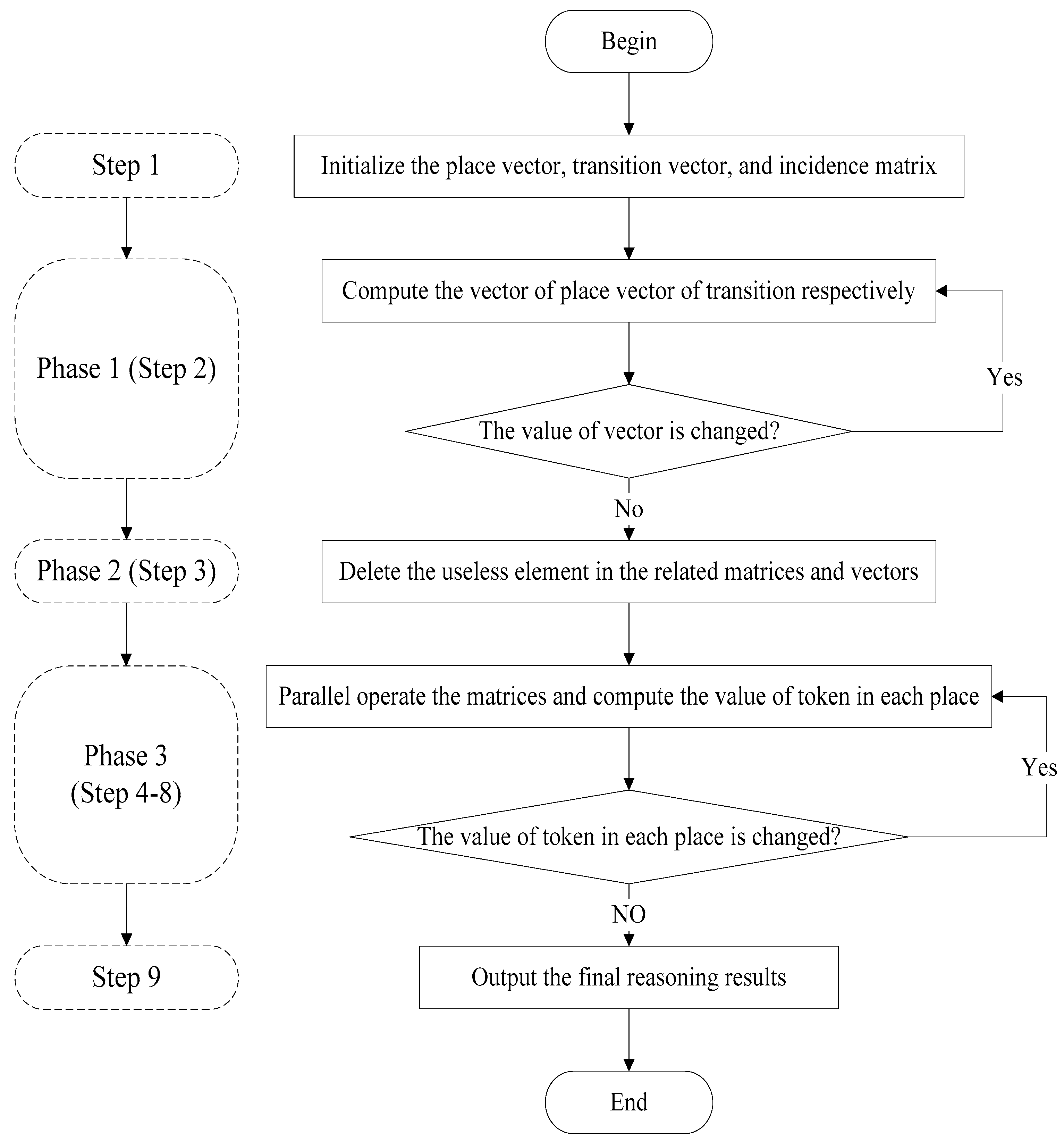
3.1. The Proposed Algorithm
3.2. Implementation Steps
4. Analysis
4.1. Correctness
4.2. Algorithm Complexity
- In the worst situation, all places and transitions appear in the reasoning path. This means that the backward reasoning mechanism is out of work. The algorithm complexity of the proposed algorithm is .
- In other situations, the number of unconcerned places and transitions are and , and the algorithm complexity of the proposed algorithm is .
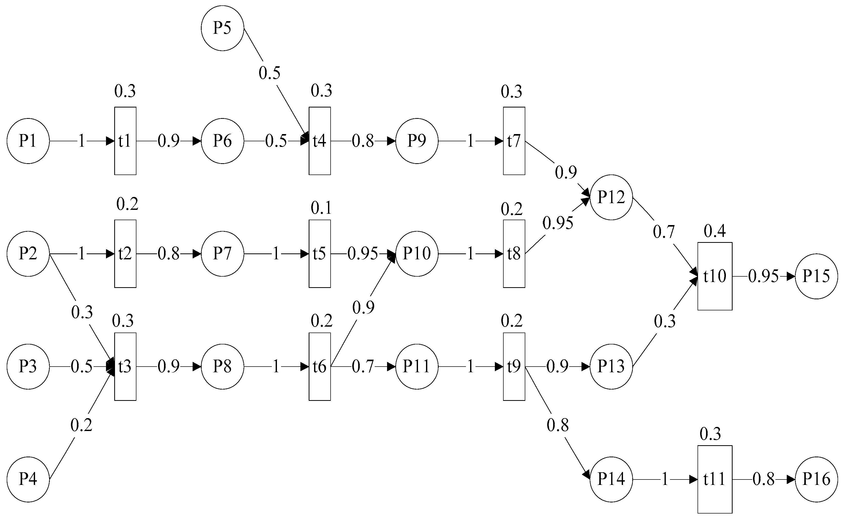
5. Case Study
5.1. Relevant Experimental Data of the Case Study
5.2. Experiments
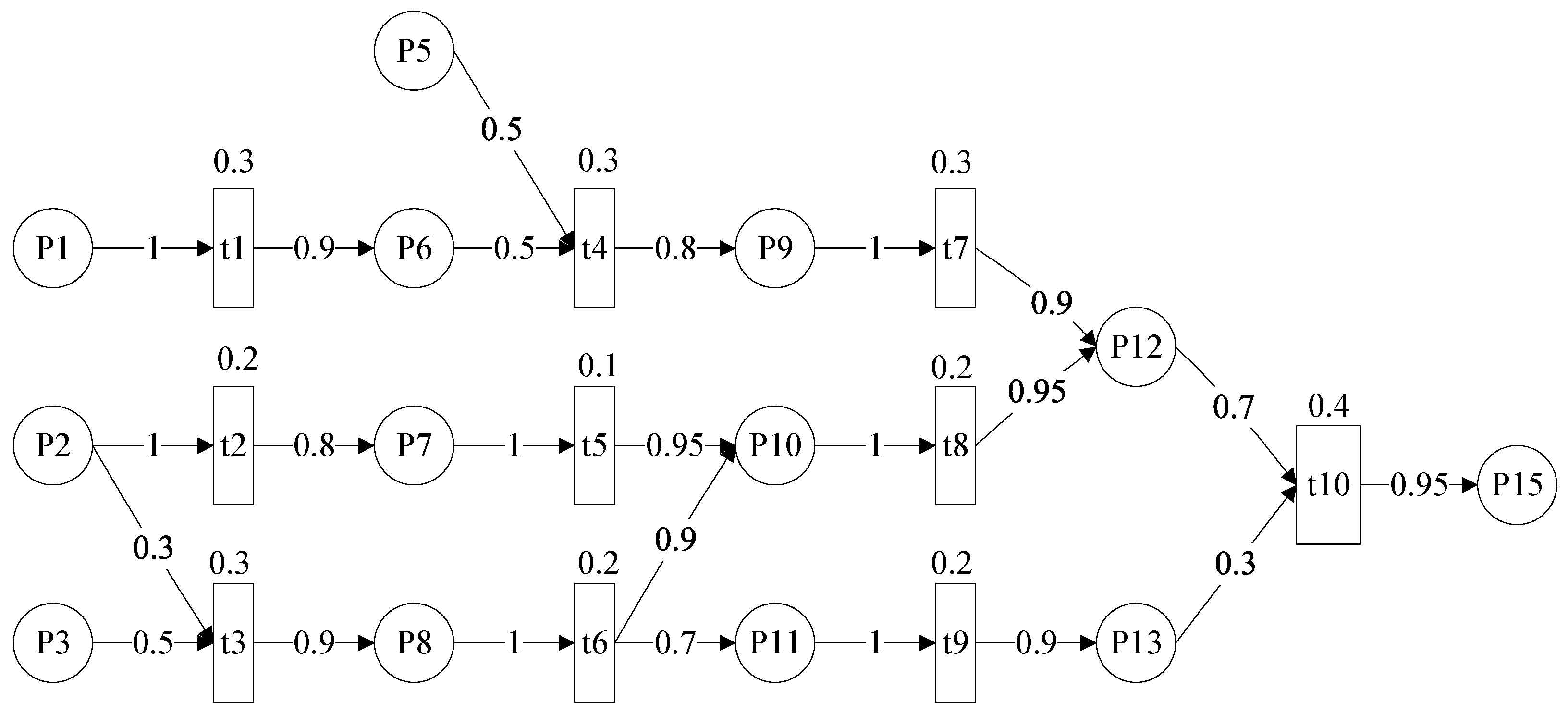
5.2.1. Experiment One
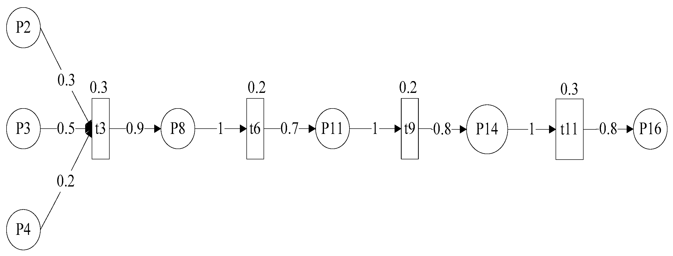
5.2.2. Experiment Two
5.3. Analysis of Experiments 1 and 2
6. Conclusions
Author Contributions
Acknowledgments
Conflicts of Interest
References
- Burrell, P.; Inman, D. An expert system for the analysis of faults in an electricity supply network: Problems and achievements. Comput. Ind. 1998, 37, 113–123. [Google Scholar] [CrossRef]
- Liu, S.C.; Liu, S.Y. An efficient expert system for machine fault diagnosis. Int. J. Adv. Manuf. Technol. 2003, 21, 691–698. [Google Scholar] [CrossRef]
- Liu, H.; Gegov, A.; Cocea, M. Rule-based systems: A granular computing perspective. Granul. Comput. 2016, 1, 259–274. [Google Scholar] [CrossRef]
- Ahmad, S.S.S.; Pedrycz, W. The development of granular rule-based systems: A study in structural model compression. Granul. Comput. 2017, 2, 1–12. [Google Scholar] [CrossRef]
- Huang, Y.; McMurran, R.; Dhadyalla, G.; Jones, R.P. Probability based vehicle fault diagnosis: Bayesian network method. J. Intell. Manuf. 2008, 19, 301–311. [Google Scholar] [CrossRef]
- Alessandri, A. Fault diagnosis for nonlinear systems using a bank of neural estimators. Comput. Ind. 2003, 52, 271–289. [Google Scholar] [CrossRef]
- Chen, K.Y.; Lim, C.P.; Lai, W.K. Application of a neural fuzzy system with rule extraction to fault detection and diagnosis. J. Intell. Manuf. 2005, 16, 679–691. [Google Scholar] [CrossRef]
- Lai, Y.F.; Chen, M.Y.; Chiang, H.S. Constructing the lie detection system with fuzzy reasoning approach. Granul. Comput. 2017, 3, 169–176. [Google Scholar] [CrossRef]
- Lukovac, V.; Pamučar, D.; Popović, M.; Đorović, B. Portfolio model for analyzing human resources: An approach based on neuro-fuzzy modeling and the simulated annealing algorithm. Expert Syst. Appl. 2017, 90, 318–331. [Google Scholar] [CrossRef]
- Pamučar, D.; Ljubojević, S.; Kostadinović, D.; Đorović, B. Cost and risk aggregation in multi-objective route planning for hazardous materials transportation—A neuro-fuzzy and artificial bee colony approach. Expert Syst. Appl. 2016, 65, 1–15. [Google Scholar] [CrossRef]
- Pamučar, D.; Vasin, L.; Atanasković, P.; Miličić, M. Planning the City Logistics Terminal Location by Applying the Green-Median Model and Type-2 Neurofuzzy Network. Comput. Intell. Neurosci. 2016, 2016, 6972818. [Google Scholar]
- Mortada, M.A.; Yacout, S.; Lakis, A. Fault diagnosis in power transformers using multi-class logical analysis of data. J. Intell. Manuf. 2013, 25, 1429–1439. [Google Scholar] [CrossRef]
- Reyes, A.; Yu, H.; Kelleher, G.; Lloyd, S. Integrating Petri Nets and hybrid heuristic search for the scheduling of FMS. Comput. Ind. 2002, 47, 123–138. [Google Scholar] [CrossRef]
- Cecil, J.A.; Srihari, K.; Emerson, C.R. A review of Petri-net applications in manufacturing. Int. J. Adv. Manuf. Technol. 1992, 7, 168–177. [Google Scholar] [CrossRef]
- Luo, X.; Kezunovic, M. Implementing fuzzy Reasoning Petri-Nets for fault section estimation. IEEE Trans. Power Deliv. 2008, 23, 676–685. [Google Scholar] [CrossRef]
- Hu, H.; Li, Z.; Al-Ahmari, A. Reversed fuzzy Petri nets and their application for fault diagnosis. Comput. Ind. Eng. 2011, 60, 505–510. [Google Scholar] [CrossRef]
- Yang, B.; Li, H. A novel dynamic timed fuzzy Petri nets modeling method with applications to industrial processes. Expert Syst. Appl. 2018, 97, 276–289. [Google Scholar] [CrossRef]
- Pan, H.L.; Jiang, W.R.; He, H.H. The Fault Diagnosis Model of Flexible Manufacturing System Workflow Based on Adaptive Weighted Fuzzy Petri Net. Adv. Sci. Lett. 2012, 11, 811–814. [Google Scholar] [CrossRef]
- Amin, M.; Shebl, D. Reasoning dynamic fuzzy systems based on adaptive fuzzy higher order Petri nets. Inf. Sci. 2014, 286, 161–172. [Google Scholar] [CrossRef]
- Liang, W.; An, R. Unobservable fuzzy petri net diagnosis technique. Aircr. Eng. Aerosp. Technol. 2013, 85, 215–221. [Google Scholar]
- Liu, H.C.; Lin QL Ren, M.L. Fault diagnosis and cause analysis using fuzzy evidential reasoning approach and dynamic adaptive fuzzy Petri nets. Comput. Ind. Eng. 2013, 66, 899–908. [Google Scholar] [CrossRef]
- Wang, W.M.; Peng, X.; Zhu, G.N.; Hu, J.; Peng, Y.H. Dynamic representation of fuzzy knowledge based on fuzzy petri net and genetic-particle swarm optimization. Expert Syst. Appl. 2014, 41, 1369–1376. [Google Scholar] [CrossRef]
- Liu, H.C.; You, J.X.; Tian, G. Determining Truth Degrees of Input Places in Fuzzy Petri Nets. IEEE Trans. Syst. Man Cyber. Syst. 2017, 47, 3425–3431. [Google Scholar] [CrossRef]
- Looney, C. G Fuzzy Petri nets for rule-based decision making. IEEE Trans. Syst. Man Cyber. 1988, 18, 178–183. [Google Scholar] [CrossRef]
- Zhou, K.Q.; Zain, A.M. Fuzzy Petri Nets and Industrial Applications: A Review. Artif. Intell. Rev. 2016, 45, 405–446. [Google Scholar] [CrossRef]
- Chen, S.M. Weighted fuzzy reasoning using Weighted Fuzzy Petri Nets. IEEE Trans. Knowl. Data Eng. 2002, 14, 386–397. [Google Scholar] [CrossRef]
- Liu, Z.; Li, H.; Zhou, P. Towards timed fuzzy Petri net algorithms for chemical abnormality monitoring. Expert Syst. Appl. 2011, 38, 9724–9728. [Google Scholar] [CrossRef]
- Wai, R.J.; Liu, C.M. Design of dynamic petri recurrent fuzzy neural network and its application to path-tracking control of nonholonomic mobile robot. IEEE Trans. Ind. Electron. 2009, 56, 2667–2683. [Google Scholar]
- Chen, S.M.; Ke, J.S.; Chang, J.F. Knowledge representation using fuzzy Petri nets. IEEE Trans. Knowl. Data Eng. 1990, 2, 311–319. [Google Scholar] [CrossRef]
- Gao, M.M.; Wu, Z.M.; Zhou, M.C. A Petri net-based formal reasoning algorithm for fuzzy production rule-based systems. IEEE Int. Conf. Syst. Man Cyber. 2000, 4, 3093–3097. [Google Scholar]
- Gao, M.M.; Zhou, M.C.; Huang, X.G.; Wu, Z.M. Fuzzy reasoning Petri nets. IEEE Trans. Syst. Man Cyber. Part A Syst. Hum. 2003, 33, 314–324. [Google Scholar]
- Liu, H.C.; Luan, X.; Li, Z.; Wu, J. Linguistic Petri Nets Based on Cloud Model Theory for Knowledge Representation and Reasoning. IEEE Trans. Knowl. Data Eng. 2018, 30, 717–728. [Google Scholar] [CrossRef]
- Guo, Y.; Meng, X.; Wang, D.; Meng, T.; Liu, S.; He, R. Comprehensive risk evaluation of long-distance oil and gas transportation pipelines using a fuzzy petri net model. J. Nat. Gas Sci. Eng. 2016, 33, 18–29. [Google Scholar] [CrossRef]
- Li, H.; You, J.X.; Liu, H.C.; Tian, G. Acquiring and Sharing Tacit Knowledge Based on Interval 2-Tuple Linguistic Assessments and Extended Fuzzy Petri Nets. Int. J. Uncertain. Fuzziness Knowl.-Based Syst. 2018, 26, 43–65. [Google Scholar] [CrossRef]
- Zhou, K.Q.; Zain, A.M.; Mo, L.P. A decomposition algorithm of fuzzy Petri net using an index function and incidence matrix. Expert Syst. Appl. 2015, 42, 3980–3990. [Google Scholar] [CrossRef]
- Zhou K, Q.; Mo L, P.; Jin, J.; Zain, A.M. An equivalent generating algorithm to model fuzzy Petri net for knowledge-based system. J. Intell. Manuf. 2017, 1–12. [Google Scholar] [CrossRef]
- Liu, H.C.; You, J.X.; Li, Z.; Tian, G. Fuzzy Petri nets for knowledge representation and reasoning: A literature review. Eng. Appl. Artif. Intell. 2017, 60, 45–56. [Google Scholar] [CrossRef]
- Zhang, J.H.; Xia, J.J.; Garibaldi, J.M.; Groumpos, P.P.; Wang, R.B. Modeling and control of operator functional state in a unified framework of fuzzy inference petri nets. Comput. Methods Prog. Biomed. 2017, 144, 147–163. [Google Scholar] [CrossRef] [PubMed]
- Nazareth, D.L. Investigating the applicability of Petri nets for rule-based system verification. IEEE Trans. Knowl. Data Eng. 1993, 5, 402–415. [Google Scholar] [CrossRef]


| Place | Meaning |
|---|---|
| P1 | molecular pump is not in proper position |
| P2 | pressure exerted is too high |
| P3 | temperature of cooling water is high |
| P4 | cooling system failures |
| P5 | pump is not drying enough |
| P6 | air exhaust is not enough |
| P7 | compressor operates in magnetic field |
| P8 | roller bearing wears |
| P9 | compressor is noisy |
| P10 | temperature of bump is high |
| P11 | blade of turbine wears |
| P12 | blade of compressor is broken |
| P13 | pressurization ratio of compressor is low |
| P14 | blade of turbine is scales |
| P15 | compressor is in turbulence |
| P16 | blade of turbine breaks down |
| Repeat | Output Strength Vector |
|---|---|
| 1st | |
| 2nd | |
| 3rd | |
| 4th | |
| 5th |
| Repeat | M′ |
|---|---|
| 1st | |
| 2nd | |
| 3rd | |
| 4th | |
| 5th |
| Repeat | Output Strength Vector |
|---|---|
| 1st | |
| 2nd | |
| 3rd | |
| 4th | |
| 5th |
| Repeat | M′ |
|---|---|
| 1st | |
| 2nd | |
| 3rd | |
| 4th | |
| 5th |
| Related Matrices | Experiment One | Experiment Two | |
|---|---|---|---|
| Original Matrices | , and | 16 × 11 | 16 × 11 |
| 11 × 16 | 11 × 16 | ||
| In backward reasoning phase | and | 16 × 11 | 16 × 11 |
| 11 × 16 | 11 × 16 | ||
| In forward reasoning phase | and | 14 × 10 | 7 × 4 |
| 10 × 14 | 4 × 7 |
© 2018 by the authors. Licensee MDPI, Basel, Switzerland. This article is an open access article distributed under the terms and conditions of the Creative Commons Attribution (CC BY) license (http://creativecommons.org/licenses/by/4.0/).
Share and Cite
Zhou, K.-Q.; Gui, W.-H.; Mo, L.-P.; Zain, A.M. A Bidirectional Diagnosis Algorithm of Fuzzy Petri Net Using Inner-Reasoning-Path. Symmetry 2018, 10, 192. https://doi.org/10.3390/sym10060192
Zhou K-Q, Gui W-H, Mo L-P, Zain AM. A Bidirectional Diagnosis Algorithm of Fuzzy Petri Net Using Inner-Reasoning-Path. Symmetry. 2018; 10(6):192. https://doi.org/10.3390/sym10060192
Chicago/Turabian StyleZhou, Kai-Qing, Wei-Hua Gui, Li-Ping Mo, and Azlan Mohd Zain. 2018. "A Bidirectional Diagnosis Algorithm of Fuzzy Petri Net Using Inner-Reasoning-Path" Symmetry 10, no. 6: 192. https://doi.org/10.3390/sym10060192
APA StyleZhou, K.-Q., Gui, W.-H., Mo, L.-P., & Zain, A. M. (2018). A Bidirectional Diagnosis Algorithm of Fuzzy Petri Net Using Inner-Reasoning-Path. Symmetry, 10(6), 192. https://doi.org/10.3390/sym10060192