Some Results on the Graph Theory for Complex Neutrosophic Sets

 ,
, 
Abstract
:1. Introduction
2. Preliminaries
- (i)
- The union of and , denoted as , is defined as:where are given by:
- (ii)
- The intersection of and , denoted as is defined as:where are given by:
- (a)
- Sum:
- (b)
- Max:
- (c)
- Min:
- (d)
- “The game of winner, neutral, and loser”:
- (a)
- is a non-void set.
- (b)
- , , are three functions, each from to [0, 1].
- (c)
- , , are three functions, each from to [0, 1].
- (d)
- and .
- (i)
- depends on and depends on , , Hence there are seven mutually independent parameters in total that make up a CNG1: , , .
- (ii)
- For each is said to be a vertex of The entire set is thus called the vertex set of
- (iii)
- For each is said to be a directed edge of In particular, is said to be a loop of
- (iv)
- For each vertex: are called the truth-membership value, indeterminate membership value, and false-membership value, respectively, of that vertex Moreover, if then is said to be a void vertex.
- (v)
- Likewise, for each edge are called the truth-membership value, indeterminate-membership value, and false-membership value, respectively of that directed edge Moreover, if then is said to be a void directed edge.
- (a)
- is a non-void set.
- (b)
- is a function from to .
- (c)
- is a function from to .
- (i)
- the structure is said to be a complex fuzzy graph of type 1 (abbr. CFG1).
- (ii)
- For each , is said to be a vertex of . The entire set is thus called the vertex set of .
- (iii)
- For each , is said to be a directed edge of . In particular, is said to be a loop of .
3. Complex Neutrosophic Graphs of Type 1
- (a)
- is a non-void set.
- (b)
- , , are three functions, each from to .
- (c)
- , , are three functions, each from to .
- (d)
- and .
- (i)
- For each , is said to be a vertex of . The entire set is thus called the vertex set of .
- (ii)
- For each , is said to be a directed edge of . In particular, is said to be a loop of .
- (iii)
- For each vertex: , , are called the complex truth, indeterminate, and falsity membership values, respectively, of the vertex . Moreover, if = = = 0, then is said to be a void vertex.
- (iv)
- Likewise, for each directed edge are called the complex truth, indeterminate and falsity membership value, of the directed edge . Moreover, if then is said to be a void directed edge.
- (a)
- If , then is said to be an (ordinary) edge of . Moreover, is said to be a void (ordinary) edge if both and are void.
- (b)
- If holds for all then is said to be ordinary (or undirected), otherwise it is said to be directed.
- (c)
- If all the loops of are void, then is said to be simple.
- (a)
- is said to be adjacent to (and to ).
- (b)
- (and as well) is said to be an end-point of .
3.1. The Scenario
- (i)
- When or access the internet together, they will simply search for “a place of common interest”. This is regardless of who initiates the invitation.
- (ii)
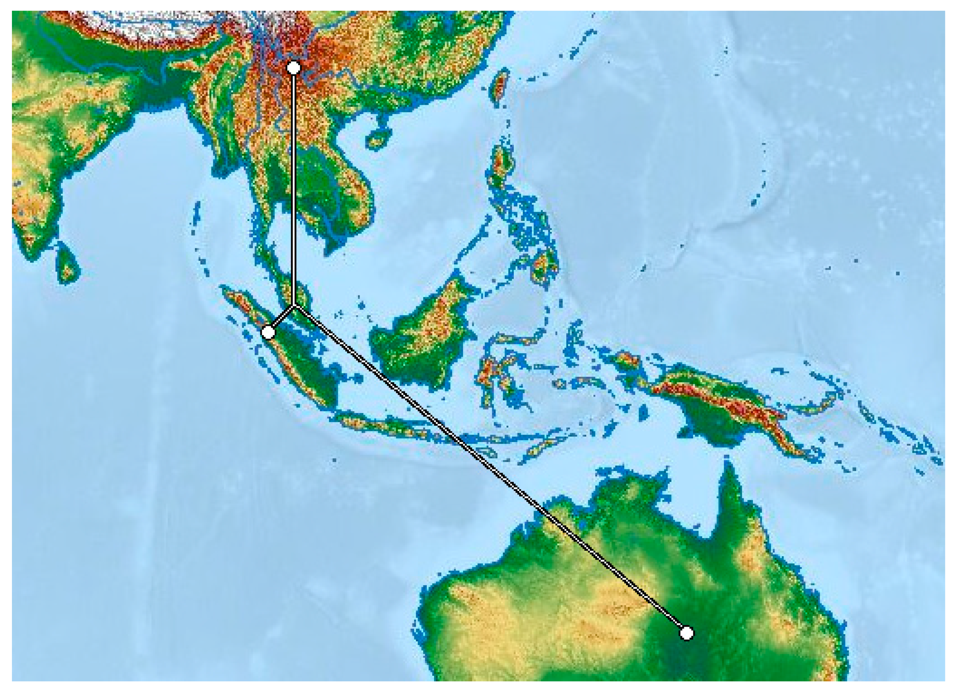
- and rarely meet. Thus, each time they do, everyone (especially the children) will be so excited that they would like to try something fresh, so all will seek excitement and connect towards to a local broadcasting server at 240° to watch soccer matches (that server will take care of which country to connect to) for the entire day. This is also regardless of who initiates the visitation.
- (iii)
- The size and the wealth of far surpasses Thus, it would always be who invites to their house, never the other way, and during the entire visit, members of will completely behave like members of and, therefore, will visit the same websites as .
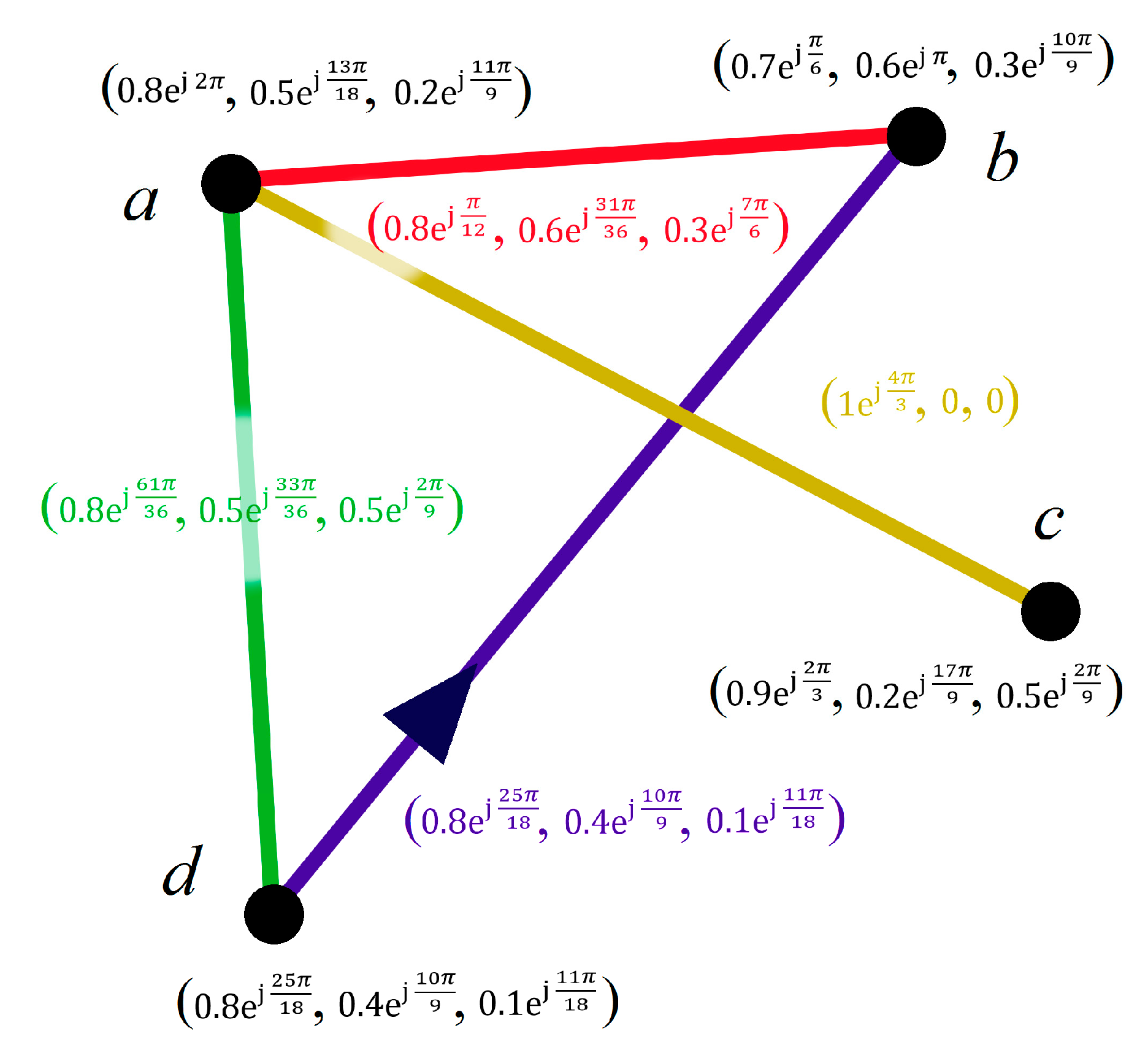
3.2. Representation of the Scenario with CNG1
- (a)
- Take V0 = .
- (b)
- In accordance with the scenario, define the three functions on V0: , , , as illustrated in Table 3.
- (c)
- (d)
- By statement (d) from Definition 7, let = (, , ), and = (, , ). We have now formed a CNG1
4. Representation of a CNG1 by an Adjacency Matrix
4.1. Two Methods of Representation
4.2. Illustrative Example
5. Some Theoretical Results on Ordinary CNG1
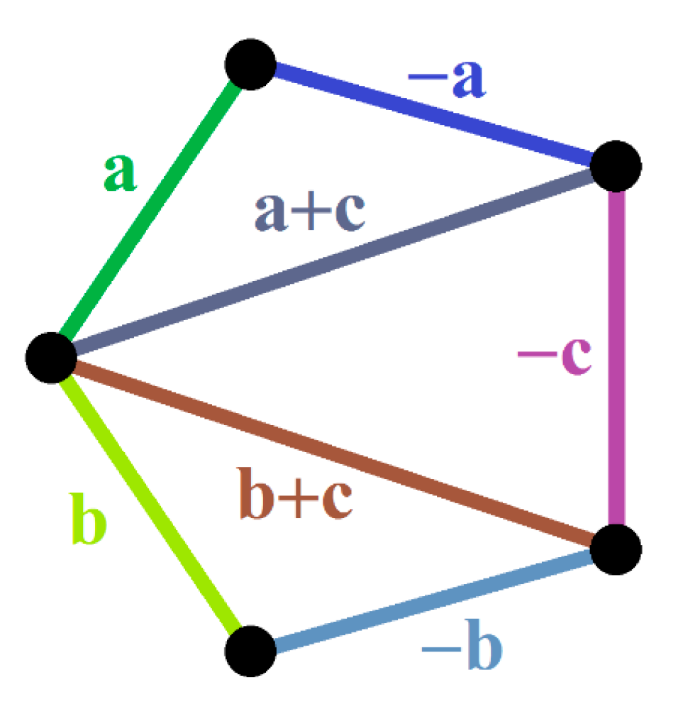
- (a)
- = + ,
- (b)
- = + ,
- (c)
- = + .
- (a)
- = ,
- (b)
- = ,
- (c)
- = .
- (a)
- = + ,
- (b)
- = + ,
- (c)
- = + .
- (a)
- = ,
- (b)
- = ,
- (c)
- = .
- (a)
- = + ,
- (b)
- = + ,
- (c)
- = + .
- (a)
- = ,
- (b)
- = ,
- (c)
- = .
- (a)
- = + ,
- (b)
- = + ,
- (c)
- = + .
- (a)
- = ,
- (b)
- = ,
- (c)
- = .
- = = ,
- = = ,
- = = ,
6. The Shortest CNG1 of Certain Conditions
- (a)
- is simple.
- (b)
- is connected.
- (c)
- for all , = and = .
- (a)
- and .
- (b)
- and .
- (c)
- and .
- (a)
- (most “widely spread” possibility)
- (b)
- (c)
- (most “concentrated” possibility)
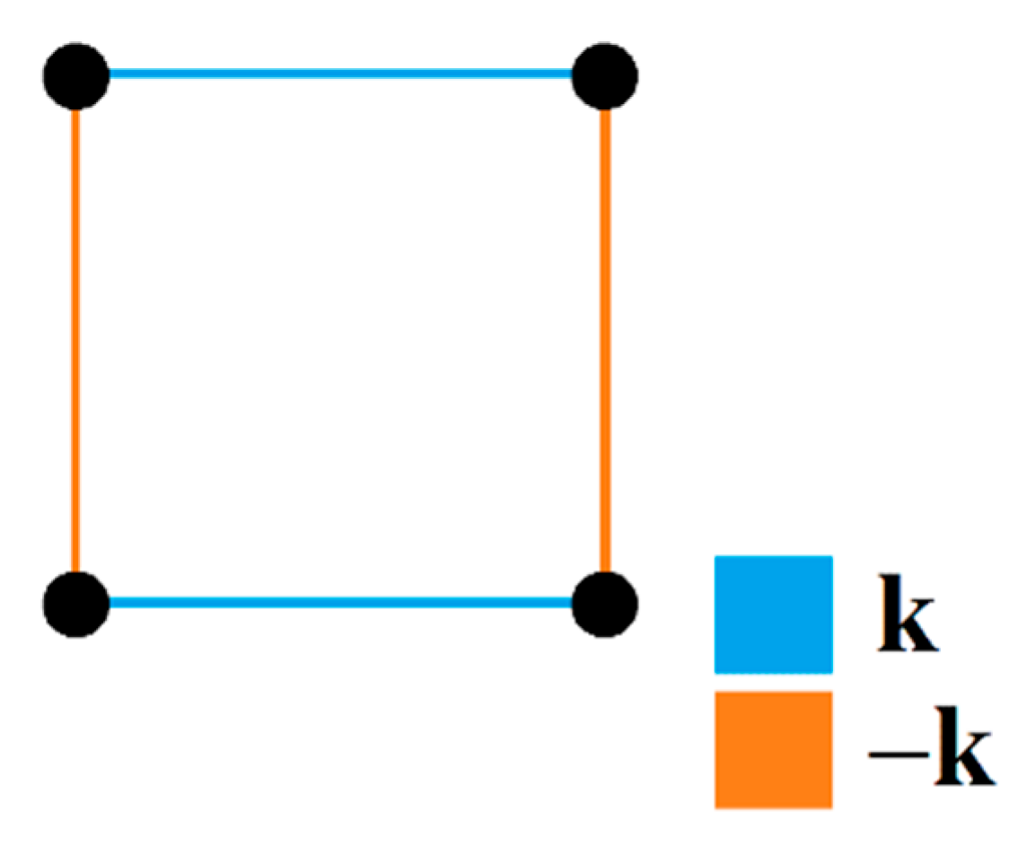
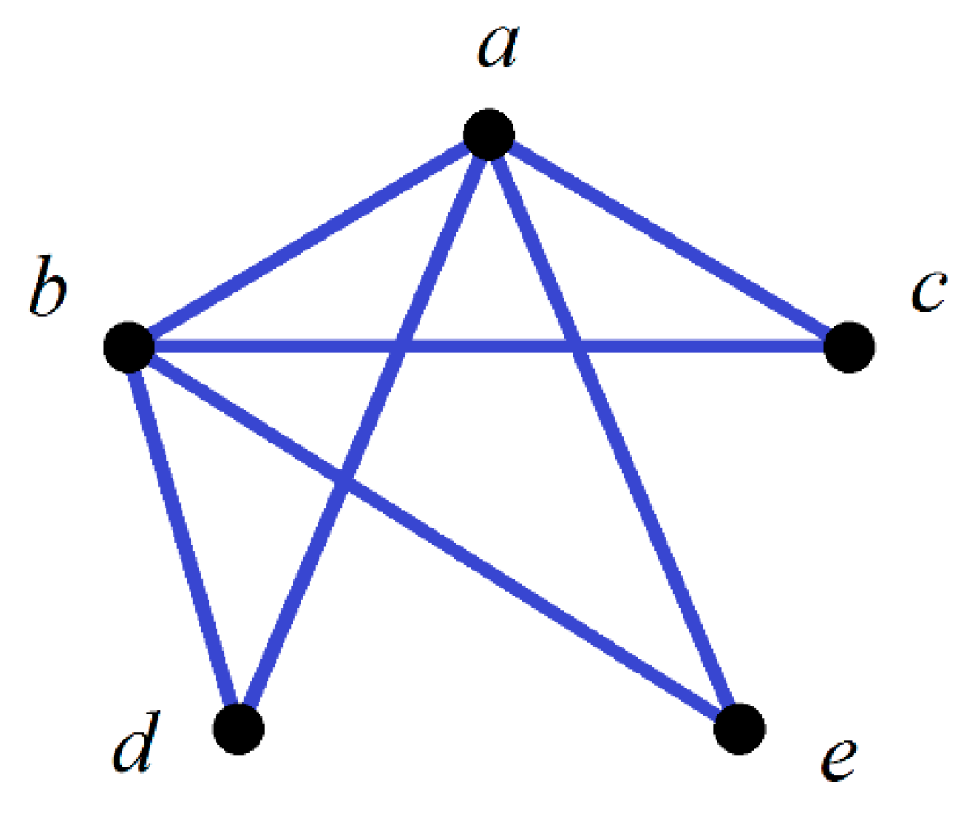
7. Symmetric Properties of Ordinary Simple CNG1
- (a)
- for all .
- (b)
- for all .
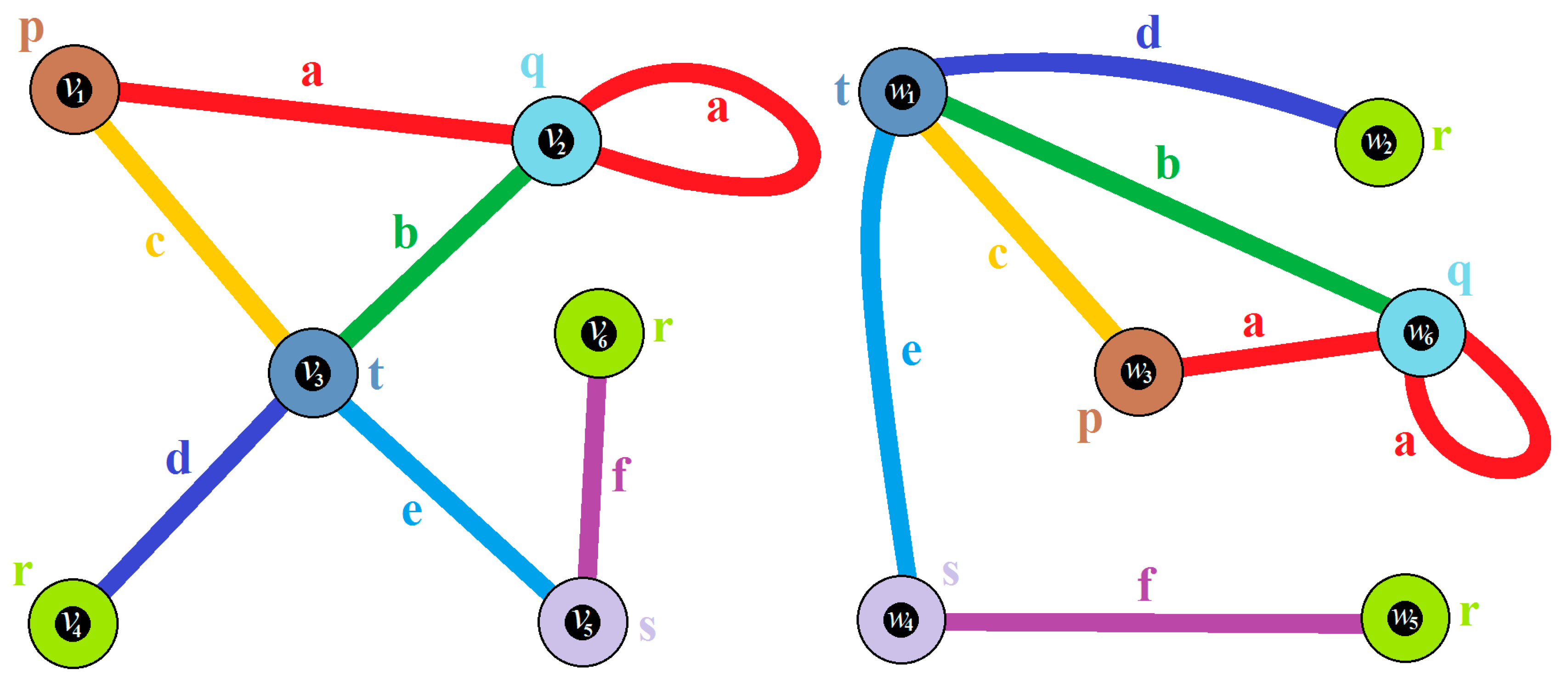
- (i)
- Such is said to be an isomorphism from to , and we shall denote such case by .
- (ii)
- and are said to be isomorphic, and shall be denoted by .
- (a)
- for all .
- (b)
- for all .
- (a)
- .
- (b)
- .
- (c)
- .
- (i)
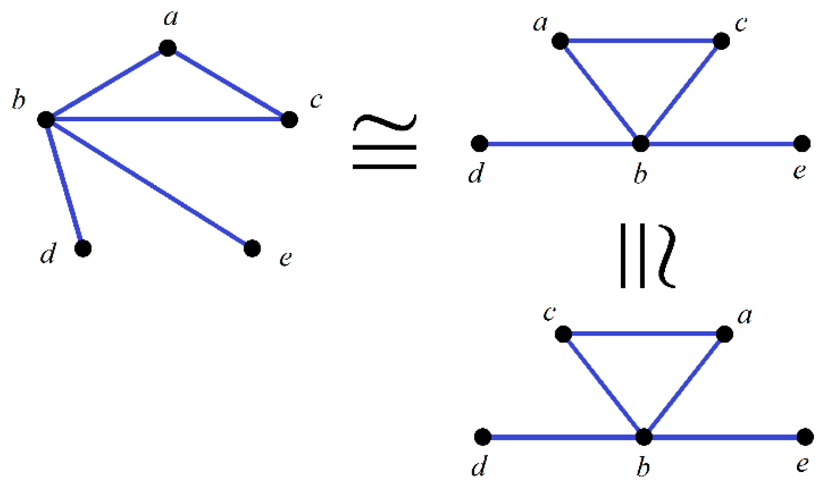
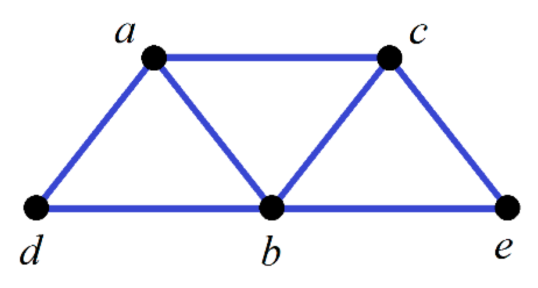
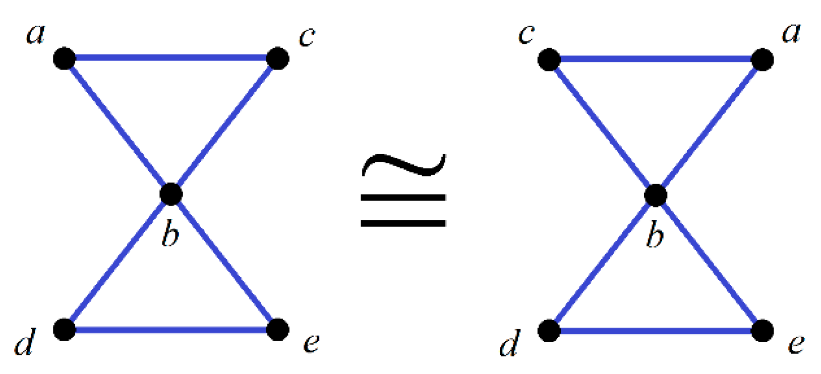
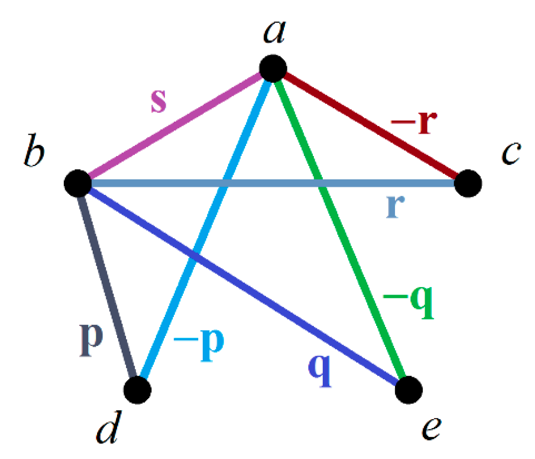
- is an isomorphism from to the following ordinary CNG1 (Figure 21).which is not equal to in accordance with Definition 18. is therefore not an automorphism of .
- (ii)
- is an isomorphism from to the following ordinary CNG1 (Figure 22).which is also not equal to in accordance with Definition 18. Likewise is, therefore, not an automorphism of .
- (iii)
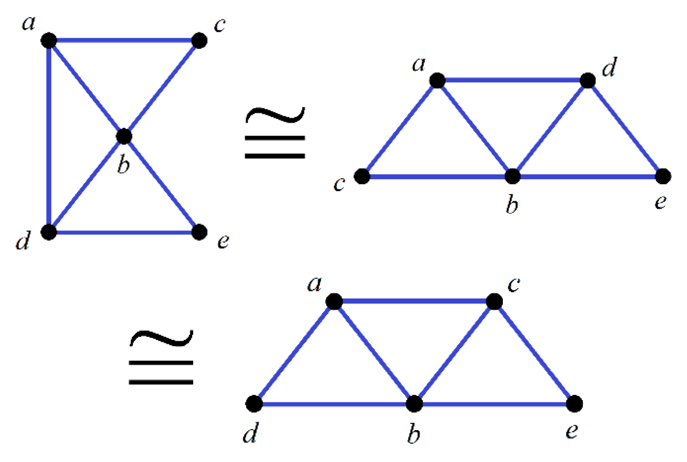
- is an isomorphism from to itself and, therefore, it is an automorphism of . Note that, even if and , as and , so still holds.
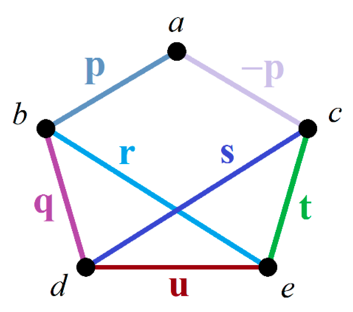
- (a)
- ,
- (b)
- ,
- (c)
- ,
8. Conclusions
Author Contributions
Funding
Acknowledgments
Conflicts of Interest
References
- Smarandache, F. Neutrosophic Probability, Set, and Logic; ProQuest Information & Learning: Ann Arbor, MI, USA, 1998; 105p. [Google Scholar]
- Zadeh, L.A. Fuzzy sets. Inform. Control 1965, 8, 338–353. [Google Scholar] [CrossRef]
- Atanassov, K.T. Intuitionistic fuzzy sets. Fuzzy Sets Syst. 1986, 20, 87–96. [Google Scholar] [CrossRef]
- Turksen, I. Interval valued fuzzy sets based on normal forms. Fuzzy Sets Syst. 1986, 20, 191–210. [Google Scholar] [CrossRef]
- Wang, H.; Smarandache, F.; Zhang, Y.; Sunderraman, R. Single valued neutrosophic sets. Multispace Multistruct. 2010, 4, 410–413. [Google Scholar]
- Neutrosophic Set Theory. Available online: http://fs.gallup.unm.edu/NSS/ (accessed on 1 December 2017).
- Shannon, A.; Atanassov, K. A first step to a theory of the intuitionistic fuzzy graphs. In Proceedings of the First Workshop on Fuzzy Based Expert Systems, Sofia, Bulgaria, 28–30 September 1994; Akov, D., Ed.; 1994; pp. 59–61. [Google Scholar]
- Smarandache, F. Symbolic Neutrosophic Theory; Europanova Asbl: Brussels, Belgium, 2015. [Google Scholar]
- Smarandache, F. Refined literal indeterminacy and the multiplication law of sub-indeterminacies. Neutrosophic Sets Syst. 2015, 9, 58–63. [Google Scholar]
- Smarandache, F. Types of Neutrosophic Graphs and neutrosophic Algebraic Structures together with their Applications in Technology. In Proceedings of the Seminar UniversitateaTransilvania din Brasov, Facultatea de Design de ProdussiMediu, Brasov, Romania, 6 June 2015. [Google Scholar]
- Smarandache, F. (Ed.) Neutrosophic overset, neutrosophic underset, neutrosophic offset. In Similarly for Neutrosophic Over-/Under-/Off-Logic, Probability, and Statistics; Pons Editions: Brussels, Belgium, 2016; pp. 158–168. [Google Scholar]
- Broumi, S.; Talea, M.; Bakali, A.; Smarandache, F. Single valued neutrosophic graphs. J. New Theory 2016, 10, 86–101. [Google Scholar]
- Broumi, S.; Talea, M.; Smarandache, F.; Bakali, A. Single valued neutrosophic graphs: Degree, order and size. In Proceedings of the IEEE International Conference on Fuzzy Systems, Vancouver, BC, Canada, 24–29 July 2016; IEEE: Piscataway, NJ, USA, 2016; pp. 2444–2451. [Google Scholar]
- Broumi, S.; Bakali, A.; Talea, M.; Hassan, A.; Smarandache, F. Isolated single valued neutrosophic graphs. Neutrosophic Sets Syst. 2016, 11, 74–78. [Google Scholar]
- Smarandache, F. (Ed.) Nidus idearum. In Scilogs, III: Viva la Neutrosophia; Pons asbl: Brussels, Belgium, 2017; ISBN 978-1-59973-508-5. [Google Scholar]
- Samanta, S.; Sarkar, B.; Shin, D.; Pal, M. Completeness and regularity of generalized fuzzy graphs. SpringerPlus 2016, 5, 1–14. [Google Scholar] [CrossRef] [PubMed]
- Broumi, S.; Bakali, A.; Talea, M.; Hassan, A.; Smarandache, F. Generalized single valued neutrosophic graphs of first type. In Proceedings of the 2017 IEEE International Conference on Innovations in Intelligent Systems and Applications (INISTA), Gdynia Maritime University, Gdynia, Poland, 3–5 July 2017; pp. 413–420. [Google Scholar]
- Ramot, D.; Menahem, F.; Gideon, L.; Abraham, K. Complex Fuzzy Set. IEEE Trans. Fuzzy Syst. 2002, 10, 171–186. [Google Scholar] [CrossRef]
- Selvachandran, G.; Maji, P.K.; Abed, I.E.; Salleh, A.R. Complex vague soft sets and its distance measures. J. Intell. Fuzzy Syst. 2016, 31, 55–68. [Google Scholar] [CrossRef]
- Selvachandran, G.; Maji, P.K.; Abed, I.E.; Salleh, A.R. Relations between complex vague soft sets. Appl. Soft Comp. 2016, 47, 438–448. [Google Scholar] [CrossRef]
- Kumar, T.; Bajaj, R.K. On complex intuitionistic fuzzy soft sets with distance measures and entropies. J. Math. 2014, 2014, 1–12. [Google Scholar] [CrossRef]
- Alkouri, A.; Salleh, A. Complex intuitionistic fuzzy sets. AIP Conf. Proc. 2012, 1482, 464–470. [Google Scholar]
- Selvachandran, G.; Hafeed, N.A.; Salleh, A.R. Complex fuzzy soft expert sets. AIP Conf. Proc. 2017, 1830, 1–8. [Google Scholar] [CrossRef]
- Selvachandran, G.; Salleh, A.R. Interval-valued complex fuzzy soft sets. AIP Conf. Proc. 2017, 1830, 1–8. [Google Scholar] [CrossRef]
- Greenfield, S.; Chiclana, F.; Dick, S. Interval-valued Complex Fuzzy Logic. In Proceedings of the IEEE International Conference on Fuzzy Systems, Vancouver, BC, Canada, 24–29 July 2016; IEEE: Piscataway, NJ, USA, 2016; pp. 1–6. [Google Scholar]
- Ali, M.; Smarandache, F. Complex neutrosophic set. Neural Comp. Appl. 2017, 28, 1817–1834. [Google Scholar] [CrossRef]
- Thirunavukarasu, P.; Suresh, R.; Viswanathan, K.K. Energy of a complex fuzzy graph. Int. J. Math. Sci. Eng. Appl. 2016, 10, 243–248. [Google Scholar]
- Smarandache, F. A geometric interpretation of the neutrosophic set—A generalization of the intuitionistic fuzzy set. In Proceedings of the IEEE International Conference on Granular Computing, National University of Kaohsiung, Kaohsiung, Taiwan, 8–10 November 2011; Hong, T.P., Kudo, Y., Kudo, M., Lin, T.Y., Chien, B.C., Wang, S.L., Inuiguchi, M., Liu, G.L., Eds.; IEEE Computer Society; IEEE: Kaohsiung, Taiwan, 2011; pp. 602–606. [Google Scholar]
- Smarandache, F. Degree of dependence and independence of the (sub) components of fuzzy set and neutrosophic set. Neutrosophic Sets Syst. 2016, 11, 95–97. [Google Scholar]
- Ali, M.; Son, L.H.; Khan, M.; Tung, N.T. Segmentation of dental X-ray images in medical imaging using neutrosophic orthogonal matrices. Expert Syst. Appl. 2018, 91, 434–441. [Google Scholar] [CrossRef]
- Ali, M.; Dat, L.Q.; Son, L.H.; Smarandache, F. Interval complex neutrosophic set: Formulation and applications in decision-making. Int. J. Fuzzy Syst. 2018, 20, 986–999. [Google Scholar] [CrossRef]
- Ali, M.; Son, L.H.; Thanh, N.D.; Minh, N.V. A neutrosophic recommender system for medical diagnosis based on algebraic neutrosophic measures. Appl. Soft Comp. 2017. [Google Scholar] [CrossRef]


| Activities | ||||
|---|---|---|---|---|
| Some members will seek excitement (e.g., playing online games) | Happens on 80% of the day, and those will be connecting towards 0° (because that server is located in China ) | Happens on 70% of the day, and those will be connecting towards 30° | Happens on 90% of the day, and those will be connecting towards 120° | Happens on 80% of the day, and those will be connecting towards 250° |
| Some members will want to surf around (e.g., online shopping) | Happens on 50% of the day, and those will be connecting towards 130° (because that server is located in Australia ) | Happens on 60% of the day, and those will be connecting towards 180° | Happens on 20% of the day, and those will be connecting towards 340° | Happens on 40% of the day, and those will be connecting towards 200° |
| Some members will need to relax (e.g., listening to music) | Happens on 20% of the day, and those will be connecting towards 220° (because that server is located in Sumatra , Indonesia) | Happens on 30% of the day, and those will be connecting towards 200° | Happens on 50% of the day, and those will be connecting towards 40° | Happens on 10% of the day, and those will be connecting towards 110° |
| Activities | , | , | , | |
|---|---|---|---|---|
| Some members will seek excitement | Happens on 80% of the day, and those will be connecting towards 15° | Happens on the entire day, all will be connecting towards 240° | Happens on 80% of the day, and those will be connecting towards 305° | Happens on 80% of the day, and those will be connecting towards 250° |
| Some members will want to surf around | Happens on 60% of the day, and those will be connecting towards 155° | Does not happen | Happens on 50% of the day, and those will be connecting towards 165° | Happens on 40% of the day, and those will be connecting towards 200° |
| Some members will need to relax | Happens on 30% of the day, and those will be connecting towards 210° | Does not happen | Happens on 50% of the day, and those will be connecting towards 40° | Happens on 10% of the day, and those will be connecting towards 110° |
| v | ||||
|---|---|---|---|---|
| k | ||||
| 0.8 | 0.7 | 0.9 | 0.8 | |
| 0.5 | 0.6 | 0.2 | 0.4 | |
| 0.2 | 0.3 | 0.5 | 0.1 |
| v | ||||
|---|---|---|---|---|
| u | ||||
| 0 | ||||
| 0 | 0 | 0 | ||
| 0 | 0 | 0 | ||
| 0 | 0 |
| v | ||||
|---|---|---|---|---|
| u | ||||
| 0 | 0 | |||
| 0 | 0 | 0 | ||
| 0 | 0 | 0 | 0 | |
| 0 | 0 |
| v | ||||
|---|---|---|---|---|
| u | ||||
| 0 | 0 | |||
| 0 | 0 | 0 | ||
| 0 | 0 | 0 | 0 | |
| 0 | 0 |
© 2018 by the authors. Licensee MDPI, Basel, Switzerland. This article is an open access article distributed under the terms and conditions of the Creative Commons Attribution (CC BY) license (http://creativecommons.org/licenses/by/4.0/).
Share and Cite
Quek, S.G.; Broumi, S.; Selvachandran, G.; Bakali, A.; Talea, M.; Smarandache, F. Some Results on the Graph Theory for Complex Neutrosophic Sets. Symmetry 2018, 10, 190. https://doi.org/10.3390/sym10060190
Quek SG, Broumi S, Selvachandran G, Bakali A, Talea M, Smarandache F. Some Results on the Graph Theory for Complex Neutrosophic Sets. Symmetry. 2018; 10(6):190. https://doi.org/10.3390/sym10060190
Chicago/Turabian StyleQuek, Shio Gai, Said Broumi, Ganeshsree Selvachandran, Assia Bakali, Mohamed Talea, and Florentin Smarandache. 2018. "Some Results on the Graph Theory for Complex Neutrosophic Sets" Symmetry 10, no. 6: 190. https://doi.org/10.3390/sym10060190
APA StyleQuek, S. G., Broumi, S., Selvachandran, G., Bakali, A., Talea, M., & Smarandache, F. (2018). Some Results on the Graph Theory for Complex Neutrosophic Sets. Symmetry, 10(6), 190. https://doi.org/10.3390/sym10060190