Abstract
A novel approach is proposed for the path tracking of a Wheeled Mobile Robot (WMR) in the presence of an unknown lateral slip. Much of the existing work has assumed pure rolling conditions between the wheel and ground. Under the pure rolling conditions, the wheels of a WMR are supposed to roll without slipping. Complex wheel-ground interactions, acceleration and steering system noise are the factors which cause WMR wheel slip. A basic research problem in this context is localization and slip estimation of WMR from a stream of noisy sensors data when the robot is moving on a slippery surface, or moving at a high speed. DecaWave based ranging system and Particle Filter (PF) are good candidates to estimate the location of WMR indoors and outdoors. Unfortunately, wheel-slip of WMR limits the ultimate performance that can be achieved by real-world implementation of the PF, because location estimation systems typically partially rely on the robot heading. A small error in the WMR heading leads to a large error in location estimation of the PF because of its cumulative nature. In order to enhance the tracking and localization performance of the PF in the environments where the main reason for an error in the PF location estimation is angular noise, two methods were used for heading estimation of the WMR (1): Reinforcement Learning (RL) and (2): Location-based Heading Estimation (LHE). Trilateration is applied to DecaWave based ranging system for calculating the probable location of WMR, this noisy location along with PF current mean is used to estimate the WMR heading by using the above two methods. Beside the WMR location calculation, DecaWave based ranging system is also used to update the PF weights. The localization and tracking performance of the PF is significantly improved through incorporating heading error in localization by applying RL and LHE. Desired trajectory information is then used to develop an algorithm for extracting the lateral slip along X- and Y-axis from the PF estimated position of the WMR, the lateral slip along X- and Y-axis is then used to take some corrective measures. Lateral slip information is also used to find the direction along which WMR has to move to get back along the desired trajectory. Simulation results show that our proposed LHE and RL heading estimation methods significantly improve the PF localization and tracking performance on a slippery surface in both indoor and outdoor environments. The simulation results also show that the accurate locations of WMR and desired path information are used to estimate and compensate the lateral slip.
Keywords:
wheeled mobile robot (WMR); RL; DecaWave; tracking; localization; PF; tag; anchor; RTLS; wheel-slip estimation 1. Introduction
Wheeled Mobile Robot (WMR) has a broad spectrum of applications in both civilian and military engineering areas, such as search and rescue, mine clearance, scout, superstores, restaurants, and space exploration [1,2]. Wheel slip becomes a problem when the pure rolling conditions are not satisfied. Under the pure rolling assumption, the WMR’s wheels are supposed to roll without slipping. This pure rolling assumption is not satisfied when the WMR either has complex wheel-ground interactions, accelerating, decelerating, steering system has noise, or the WMR is moving on a slippery surface. Because of the above wheel slip reasons during navigation, the WMR can significantly deviate from the planned trajectory. Ignoring the effect of wheel slip may result in a larger difference between actual and command heading of the WMR, instability of tracking and localization system and a complete mission failure. So, to bridge a gap between planning and navigation, WMR slip estimation is required in order to take corrective measures afterward. There are many slip-estimation mechanisms to improve the localization, navigation, and tracking performance [3,4,5,6,7]. Inertial Measurement Unit (IMU)-based localization and slip estimation [8], fuzzy-controller and current-sensing based slip estimation [9,10], Kalman and Particle Filter based slip estimation [11,12], and vision-based slip estimation [13]. Most of the above wheel slip estimation techniques have some limitations. Vision-based slip estimation is not effective in an indoor environment because of light variation. A major disadvantage of using the IMU is, it typically suffers from accumulated error. Current-sensing based wheel slip estimation works only for longitudinal slip estimation. Furthermore, current-sensing based slip estimation requires some knowledge about the physical features of the earth surface. Kalman Filter based slip estimation is only applicable to linear systems. For indoor slippery surfaces tracking and localization of the WMR is more challenging than outdoor because of the presence of multipath fading and non-line-of-sight (NLOS) conditions. A comprehensive study is presented on design and hardware selection of robots [14,15]. Different researchers have come up with different localization technologies for indoor environment; WiFi [16], ultrasonic [17,18], RFID tags [19,20,21], FM [22], magnetic field [23,24], IMU [25], cameras, lasers and sonar [26,27]. Most of these technologies and solutions have some disadvantages and limitations especially when they are used in the indoor environment. WiFi signal strength fluctuates in a time-variant indoor environment. Vision sensors provide better performance in comparison to other types of sensors for indoor autonomous navigation of robots because of low cost, low power, high resolution and capturing ability, but they are sensitive to the light variations [28]. Ultrasonic sensors (US) are cheap, low power and small in size but they suffer from having a short range and relatively low accuracy in distance measurements [29]. Laser rangefinders provide better resolution and longer detection range but they are expensive, bulkier and harmful [30]. GPS is not considered a good solution for the indoor environment because of weak signal coverage [31]. Compared to the above technologies, localization and tracking with Ultra-Wide Band(UWB) radio technology, in an indoor environment with multipath fading and NLOS conditions, is considered to be a robust solution [32,33]. Since no localization sensor takes 100% accurate measurements, it is of immense importance, to fuse the sensed location information along with their uncertainties, from different types of sensors. Bayesian filtering is a powerful tool for handling measurement uncertainties and multi-sensor fusion [34]. One best Bayesian filtering based candidate to manage measurement uncertainty is Particle Filtering (PF). It is able to manage non-Gaussian uncertainties that typically appear in the presence of NLOS conditions [35,36], it is used for solving localization, tracking, and navigation problems [37]. PF is a Monte Carlo estimation algorithm in which a posteriori probability density function is constructed by using weighted particles to make it suitable for the state estimation of non-Gaussian systems [38]. PF is a recursive state estimation approach; it is represented by a set of discrete weighted target states, called “particles”. Based on the observation gathered, at discrete time intervals, the set of particles are updated in such a way that the particles will ideally converge on the real target state. In order to track a WMR, an estimate of the WMR’s position based on measurements of relative range and angles to its position from fixed landmarks is required. Distance (range) noise has minimal, while angular noise has an exponential impact on the localization and tracking accuracy of the PF because of its cumulative nature [39]. Therefore, a small uncertainty in angle can severely degrade localization, navigation and tracking performance of the PF.
This article proposes, (1): Location-based Heading Estimation (LHE) and (2): Reinforcement Learning (RL), for heading estimation of the Wheeled Mobile Robot (WMR) in the presence of angular noise. WMR wheel slip is incorporated in PF location estimation by applying the above two methods of heading estimation. The contributions of this work are many-folds. First, wheel slip is incorporated into the WMR location which enhances the localization and tracking performance of PF on the slippery ground surface. Secondly, low-power consumption, cheap and small form factor of integrated circuit DecaWave-based system for the ranging and heading estimation of WMR is proposed, which is a good solution for resource-constrained robots. Third, an algorithm is developed which uses the accurate location of WMR and desired path information for estimating and compensating the robot lateral slip along X- and Y-axis. The lateral slip information is used to find the direction along which WMR should move to get back to the desired path and compensate the wheel slip. Simulation results validate that our proposed system not only localize and track a WMR, which is moving on a slippery surface or at a high speed but also estimate and compensate the wheel slip. It can be used for both indoor and outdoor, slippery and sandy, ground surfaces and any other type of terrain which cause robot wheel slip. The remaining of this article is organized as follow. Section 2 explains the basic theory and background knowledge, Section 3 provides an introduction of DecaWave based Real Time Location System (RTLS), Section 4 presents the results and discussion, and finally Section 5 provides the conclusions.
2. Basic Theory and Background Knowledge
2.1. Bayes Filter
At the core of probabilistic robotics is the idea of dynamic state estimation from a noisy sensor data, that are not directly observable, but that can be inferred. In Bayes filters, a state at time k is represented by a random variables , this plays a predominant role in probabilistic robotics by inferring the real state () of the system from the observations . In location estimation problems, state is an object’s or person’s two or three dimensional location, where observations about the state are gathered from the location sensors. System state estimation means getting the state equation of the system through the observation. According to Bayes rule state-space can be represented as follow:
In the above state equation, state of the system at time k is represented by the vector , state noise vector at time is represented by , and a non-linear and time-dependent function describing the evolution of the state vector is represented by . The state vector is assumed to be unobservable or inferential. Noisy measurements () provides the information about the state, which are modeled by the equation:
In Equation (2), the measurement process is described by a non-linear and time-dependent function (), and the measurement noise vector is represented by . In a Bayesian estimation, state vector at time k is estimated from all the measurements () up to and including time k. At each point in time, a probability distribution over , called belief, , represents the uncertainty. In a Bayesian statistics, this problem can be formalized as the computation of the posterior probability distribution . This posterior probability distribution can be recursively calculated in two steps, prediction, and update. Bayes filters sequentially estimate the posterior density () over the random variable conditioned on all information contained in the noisy sensors data. Bayes rule provides a convenient way to infer the real state through the inverse of the posterior probability, , along with the prior probability . The belief is defined by the posterior density over the state space () conditioned on all noisy sensor data available at time k:
This posterior ( is contained on all the past measurements, , a sequence of discrete time observations provided by the location sensors. Because of the increased number of sensor measurements, in general, the computational complexity of such posterior densities grows exponentially over the time. Bayes filters assume that the dynamic system follow the first order Markov model, in order to make the computation tractable. According to the Markov assumption the location sensor measurements depend only on an object’s current location (Equation (4)), and that an object’s physical location at time k depends only on the previous state (Equation (5)).
Under the Markov assumption, belief in Equation (3) can be efficiently calculated without loss of information. There are two steps in the Bayesian rule, prediction, and update.
2.1.1. Prediction
Prediction process is based on the prior acquired information to predict the state. Prior probability density () of the state is calculated through the state Equation (1). The probability distribution can be thought of as a prior over the random variable before receiving the most latest observation, . In the prediction step, is calculated from the filtering distribution at time :
2.1.2. Process Updating
The updating process is modifying the prior probability density by the latest observation to obtain a posteriori density. The prior probability density is updated by the latest observation, , using the Bayes’ rule, to obtain the posterior over the random variable, . The posterior probabilities can be obtained according to prior . It is only a prediction process in the last step, and this step amends the last step of the forecast through the observation of the k moments. The posterior probability obtained by this step is then brought into the next prediction process to form a recurrence.
Generally the calculation in the prediction and update process of Bayes filtering is not feasible analytically, hence they need for approximate techniques such as Monte Carlo sampling.
2.2. Sequential Monte Carlo Estimation (Particle Filters)
Since the prediction and update steps of the optimal filtering are analytically not tractable, one has to use the approximation techniques, such as Monte Carlo sampling. The most basic Monte Carlo method used for this purpose is Sequential Importance Sampling (SIS). The state space is divided into many parts, in which the weighted particles are filled according to some probability distribution. The posterior density is empirically represented by a weighted sum of samples randomly drawn from the posterior probability distribution. Consider a sequence of independent and identically distributed random samples from a posterior distribution, then the Monte Carlo estimate (an estimation of the true posterior) is given by>
In Monte Carlo method, is defined as the Dirac function. When is very large, approximates the true posterior . In Bayesian inference, the posterior mean of a nonlinear function can be estimated as follow:
According to Monte Carlo assumption, independent random samples are drawn from to estimate the expectation as
2.3. Sequential Importance Sampling (SIS)
Since sampling from the true posterior is usually impossible, therefore the idea of Importance Sampling (IS) is used, the importance distribution is given by , hence
Where
Equation (11) can be rewritten as follow
By drawing the independent and identically distributed samples {} from , Equation (13) can be approximated by the following Equation
Equation (14) is called important function or importance density. Where
The central idea in Sequential Importance Sampling (SIS) is updating the particles and their weights in such a way that they would approximate the true posterior distribution at the next time step, n. To perform the update process, the following assumption for factorizing the importance distribution at time n, is adopted:
The posterior can also be factorized as
The importance weights can be recursively updated as given below
In the above Equation (18), observations () are gathered through the DecaWave based ranging system, which will be discussed in the following sections.
3. DecaWave-Based RTLS
A DecaWave based Real Time Location System (RTLS) was tested in an indoor environment to locate the position of a Tagged Moving Object (TMO) and update the Particle Filter (PF) weights. The RTLS is based on DecaWave (DWM1000), which benefit from the advantages of Ultra-Wide Band (UWB) radio technology, such as long-ranging, robustness in multipath environments, and low power consumption. It is also cheap and has small form factors of IC technology. It integrates antenna, clock circuitry, Radio Frequency (RF) circuitry and power management in a single module. It has a continuous 360° of visibility and nearly real-time response. Its low weight, small size, and ultra-low power transmission make it a very suitable solution for resource-constrained and mini-robots. Compared to other indoor systems, it offers high performance in noisy environments, coexists with current narrowband and wideband radio services and shows robustness for multi-path fading. The DWM1000 module is based on DecaWave’s DW1000, a multi-channel transceiver based on UWB radio communications allows very accurately time-stamping of messages as they leave from and arrive at the wireless transceiver [40,41]. It has a line of sight (LOS) 350 m and non-line of sight (NLOS) 40 m ranges in the indoor and outdoor environments, allowing it to be deployed in wireless local area network access points. This RTLS has fixed units to be configured as an “Anchor”, and the dynamic one as a “Tag”. The location of a Tagged Moving Object (TMO) is established using the 3 fixed anchors with known locations around the area in which the tag is located. It was found experimentally the established location has an average error in the range of (0–30) cm. This noisy location information is used for estimating the heading of a tagged wheeled mobile robot, which is moving on a slippery surface or moving at high speed. Beside the location estimation of a TMO, these anchors are simultaneously used as landmarks and ranging sensors to update the PF weights. Simulations results show the estimated heading used by Particle Filter (PF) improve the localization and tracking accuracy dramatically. To determine the absolute position of a TMO in 2-D, it is necessary to determine how far away it is from the 3 anchors. The distance between any anchor and Tagged Moving Object (TMO) is calculated from the Time of Flight (TOF). All TOF based systems work on the basis of determining the time it takes for a signal to propagate between a transmitter and a receiver. Once this time is known accurately then the distance between the receiver and transmitter can be determined since the speed of propagation of radio waves in the air is known. With this knowledge and some relatively simple mathematics (trilateration), it is possible to calculate the location of a TMO.
Figure 1a1 shows a simple two-dimensional fixed infrastructure of the Real-Time Location System (RTLS), with 3 anchors (, and ) and one tag (), which can be easily extended to three-dimensional. The tag () was connected to a computer through a Wifi-interface while the 3 anchors were placed at a 1-meter height from the ground in 3 corners of the square (500 cm) workspace. The anchor transmits a message to the tag () and records a time the message left its antenna . The tag receives the message and sends back a reply to all the anchors. The anchor records the time it receives the reply . The anchor then calculates the time difference T = , and distance using the formula = , where c is the speed of light in the air and and 3. The distances , and are used to calculate x and y coordinates of the tag () by using trilateration algorithm. RTLS was used to localize the Tagged Moving Object (TMO) as discussed above by calculating its x and y coordinates, the x and y were then sent by the tag through a Wifi interface and received by the computer. Several experiments were performed to observe the maximum and average localization error of Real-Time Location System (RTLS). Three anchors were placed one meter above the ground. A 500 cm and 1000 cm indoor spaces were chosen for the experiments. First a person, holding a tag in hands one meter above the ground in a 500 cm, slowly move along the diagonal line between (0, 0) cm to (500, 500) cm, the experiment was performed 5 times to know the sample accuracy of RTLS, sample values are shown in Figure 1b, by the black line. Then the anchors were placed in a 1000 cm space, and the person holding a tag in hands move along different paths with speed equal to and higher than human normal motion, sample path pattern are shown in Figure 1c–e. During the experiments a maximum value of error in was found to be about 50 cm, while the average error was found to be around 30 cm.
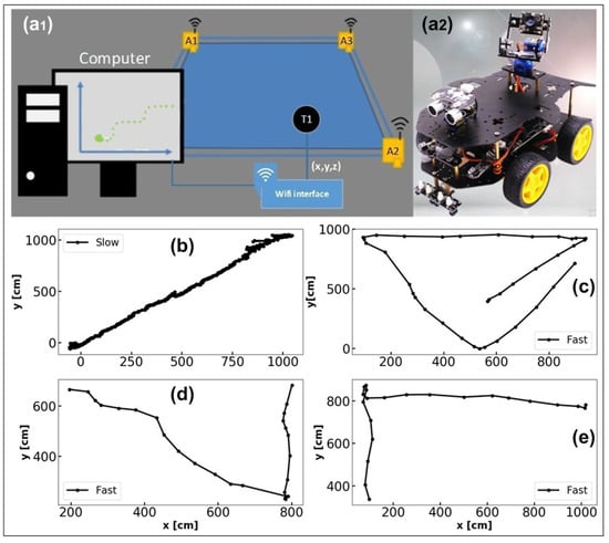
Figure 1.
(a1) Real-Time Location System (RTLS) with fixed two dimensional infrastructure, and localization of a tag () with three fixed anchors (, and ). (a2) Wheeled mobile robot (WMR) with the differential steering system; (b–e) shows a sample data from the RTLS experiments.
3.1. Wheeled Mobile Robot
We used 4-WMRs with two different types of steering systems for our experiments: (1) differential steering (DS), and (2) Ackermann steering (AS). Both types of WMRs are lightweight (about 2 kg), are battery powered, and have limited resources.
3.1.1. Differential Steering
The function of Differential Steering (DS) is achieved by applying more or less drive torque to one side of the vehicle than the other. A 4-wheeled mobile robot with a DS system that was used for the slip experiments is shown in Figure 1a2, this Wheeled Mobile Robot (WMR) can move around by 360°. It has a small camera, ultrasonic sensors, compass, and a tag; all these components are connected to a Raspberry Pi 3 board with a mini ubuntu installed on it. The tag is part of the DecaWave based ranging system discussed above. Tag establishes the real-time location of WMR with the help of fixed landmarks (anchors).
3.1.2. Ackermann Steering
The Ackermann Steering (AS) mechanism is a geometric arrangement of linkages in the steering of a vehicle designed to turn the inner and outer wheels at the appropriate angles. Features of the Ackermann based steering system robot that was used for the experiments are almost the same as the Differential based steering system robot discussed above, except the steering mechanism. Unlike the DS, AS is not very flexible to turn around 360°. During the experiments, it was observed that DS perform better than AS on a slippery ground surface.
3.2. Simulation Environment
The simulation environment is consist of; Ubuntu 16.04, Python3, and Keras with Tensorflow as a back-end. We used Turtle graphics to display simulations results on the computer screen. Keras is a high-level neural networks application programming interface, written in Python and capable of running on top of the TensorFlow.
4. Results and Discussion
The angular uncertainties have an exponential impact on the localization and tracking performance of the Particle Filter (PF); angular sensors are subjected to accumulated errors introduced by wheel slippage or other uncertainties that may perturb the course of the Wheeled Mobile Robot (WMR). When the WMR is perturbed from the desired trajectory, because of the wheel slip, the DecaWave based Real Time Location System (RTLS) is used to find its position. This position is not accurate and has some noise. Deep Q-Neural Network (DQNN) approach of Reinforcement Learning (RL) and Location-based Heading Estimation (LHE) are used to estimate heading of the WMR from the noisy location of WMR (provided by the RTLS) and the current weighted mean of the PF. PF localization accuracy is dramatically improved by the above heading estimation methods in the environment which cause WMR wheels slip. Desired path information and PF estimated the location of WMR is then used to estimate and compensate WMR’s wheel slip. Since the heading and slip estimation methods are based on location information, therefore, they are independent of the number of wheels and shape of the robot.
4.1. Distance Noise Effect on PF Performance
Weights of the particles are updated based on the distance of Wheeled Mobile Robot (WMR) to the nearest landmark (anchor). For this simulation we used 4 landmarks at (0, 0), (500, 0), (0, 500), (500, 500) in a virtual workspace of 500 cm. Noise values in the range of (0–30) cm were added in the distance of the Wheeled Mobile Robot (WMR) from the nearest landmark in accordance with the observed noise of Real-Time Location System (RTLS) discussed above. In order to measure the average error in Particle Filter Estimated Position (PFEP), the tag was allowed to move along a line between (0, 0) to (500, 500) in the workspace by making 45° angle along X-axis. The experiment was repeated several times for different values of noise added. The bar chart in Figure 2 shows errors in the moving object real position with respect to the distance uncertainty. The bar chart shows distance uncertainty has a minimal impact on PF location estimation for the following measurements. The errors have almost a linear distribution, for (0–25) cm uncertainty in the distance. The average error in moving object real position induced by the distance uncertainty was measured to be less than 6cm.
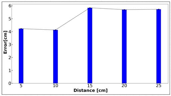
Figure 2.
Y-axis shows an average error in particle filter estimated position (PFEP) induced by the distance noise, while X-axis shows noise added in distance between moving object and the nearest landmark.
4.2. Angular Noise Effect on PF Localization Performance
Particle Filter (PF) localization performance is severely degraded by the angular noise because of its cumulative nature. To quantify the angular noise effect on PF localization performance, several computer simulations and experiments were performed. A small Wheeled Mobile Robot (WMR), which can only move forward, was used to measure the cumulative angular noise. A 10 m, indoor space was considered for the experiments and the robot was allowed to move along a path inside the workspace, the experiment was revised 10 times. It was observed that the robot has a difference of 25–30° with the initial commanded angle, which can severely degrade the localization, navigation and tracking performance of PF. Computer simulations were performed to confirm the angular noise effect on PF localization performance. As shown in Figure 5a, in the absence of angular noise robot real path (red line) is in strong correlation with its PF location estimation (green line). In Figure 5a, the commanded angle of the robot is 45° with zero angular noise, while in Figure 5b the commanded angle is 45° with 0.1° of angular noise added at each motion step. Compared to Figure 5a with the zero angular noise, in Figure 5b because of the non-zero angular noise the robot followed a curved path (red line) instead of a linear path. This is because, since PF is using 45° of angle for location estimation without knowing about the angular noise, therefore PF location estimation is severely degraded as shown in Figure 5b by the green line.
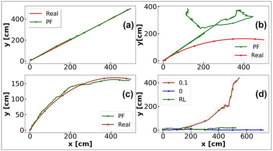
Figure 5.
The red lines show moving-object real position (MORP), while the green line shows the particle filter estimated position (PFEP) when there was (a) 0°, and (b) ° of noise added to the angle of the moving object at each motion step. (c) The red line shows MORP, while the green line shows the PFEP when reinforcement learning (RL) was used to estimate the heading from MORP with noise added to it, as well as PFEP. (d) The red line shows the exponential error growth because of cumulative angular error, the green line shows the RL angular error mitigation, and the blue line shows error in PFEP when there was 0° of error in the moving object angle.
4.3. WMR Heading Estimation with RL
To mitigate the angular noise effect on the Particle Filter (PF) localization performance we proposed Deep Q-Network (DQN) approach of Reinforcement Learning (RL) for heading estimation of Wheeled Mobile Robot (WMR), that slip because of moving on a slippery surface or sudden changes in speed. The estimated heading will incorporate the real world angular noise into the WMR position and improve the performance of Particle Filter (PF), in a drift-prone environment. A novel idea for incorporating the angular noise into the PF location estimation was introduced. Heading of the WMR was estimated from the location information using RL. The network was trained in such a way that a randomly moving object() was tracked by another moving object() by taking one of the several actions; 0: Right, 1: Top Right, 2: UP, 3: Top Left, 4: Left, 5: Bottom Left, 6: Down, 7: Bottom Right, in a two-dimensional square working space of 500 cm. A part of the 500 cm workspace is shown in Figure 3 for demonstration purpose. The actions were awarded based on the distance between and . If the distance is less than or equal to 5 cm the reward is 1000 otherwise it is −1. The output of DQN is a number from 0 to 7, as shown in Figure 4a. This output is associated with angles as (0,0/360), (1,45), (2,90), (3,135), (4,180), (5,225), (6,270) and (7,315). Neural network was used by RL as a function approximation tool for heading estimation. In RL process, a function that accepts a state s and returns the value of that state as is the value function. Similarly, there is an action-value function that accepts a state s and an action a and returns the value of taking that action given that state. After taking every action, the moving agent gets an evaluation feedback r, as well as perceives the new state. The update rule for learning state-action values is given below
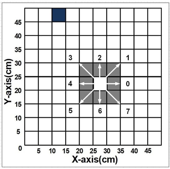
Figure 3.
White square surrounded by the gray squares is ; arrows represent the eight possible actions in a state for moving to the next state, and the dark-blue square is that needs to be tracked.
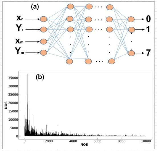
Figure 4.
(a) (, ) is a random point from a 30 cm region, (, ) is the current weighted mean of the particle filter (PF), and [0–7] is the output of Deep Q-Network (DQN). (b) Y-axis shows number of steps (NOS) in a single episode, while X-axis shows number of episodes (NOE).
In the above function, is a parameter called discount factor, it determines how much each future reward is taken into consideration for updating our Q-function. The trained network model was applied to the PF for estimating heading of the WMR. The input of DQN was taken as a random point from a 30 cm region where the robot is expected to exist, and the current weighted mean of the PF. The 30 cm region was considered in accordance with the noise pattern observation of Real-Time Location System (RTLS) discussed above. In the simulation environment, was considered as a WMR with angular noise, and was considered as a current mean of the PF. Since most of the particles will be around the PF current mean, that’s why mean is considered as to track the WMR. In the beginning, since the angular noise is not very large, the PF will use the commanded angle of the robot. As the angular noise starts to accumulate the robot starts to rely on the DQN estimated angle. After application of this DQN the cumulative angular noise was incorporated into the PF location estimation and hence the performance of the PF was dramatically improved for the conditions that cause WMR wheel slip. It’s worth mentioning, that although the neural network was trained for 500 cm region, it can be applied to any larger dimensional space by scaling the XY-coordinates of WMR and current mean positions by applying the following scaling formulas
The above expression is used when the width (w) and height (h) of the WMR’s workspace is greater than 500 cm, and are scaling factors along X- and Y-axis respectively. x and y are the coordinates of WMR and current mean of PF while and are the scaled versions of x and y.
DQN Parameters
The Deep Q-Network (DQN) discussed above, has an input layer of size 4, 4-hidden layers of sizes 200, 180, 150, 100 and an output layer of size 8 as shown in Figure 4a. The activation function of input and hidden layers is “relu” while that of the output layer is linear. The loss function is . , is a random point from a 30 cm region, which represents the position of the Wheeled Mobile Robot (WMR), , is current weighted mean of the PF, while [0–7] is the output of the DQN. is 0.95, exploration-rate is 1.0, exploration-minimum is 0.01, exploration-decay is 0.995, sample batch size is 100 and number of episodes are 10,000. Number of steps in a single episode versus the number of episodes is shown in Figure 4b. Figure 4b shows Number Of Steps (NOS) taken by to arrive the terminal state, decreases with the increased Number Of Episodes (NOE), and hence the network is converged very fast. The network training model shows that the particles around the PF mean will follow the dynamic terminal state (WMR).
Simulation results in Figure 5 show that angular error has an exponential impact on the performance of PF. Simulation results also show that the cumulative effect of angular noise can be mitigated using Reinforcement Learning (RL). A 500 cm virtual environment was considered for simulation. 0° angular noise was taken as a reference to compare the effect of cumulative angular noise, and angular noise mitigation through RL. In Figure 5a–c, the red lines show the Moving Object Real Position (MORP) and the green line shows the PF Estimated Position (PFEP). In Figure 5a, the green line shows that with a small noise in distance and no noise in the angle there is a negligibly small error in the PFEP. To show the cumulative angular noise effect on the PF accuracy, small noise of (°) was added into the robot angle and increased it by ° as the robot moves on, the angular noise is accumulated which severely degrades the location estimation performance of the PF shown by the green line in Figure 5b. Figure 5c shows that error in PFEP was mitigated using a Deep Q-Network (DQN) through estimating the heading of the moving object from location information. Figure 5d, compares, error of the cases and c respectively. In Figure 5d, the red line shows the exponential effect of the cumulative angular error on PF performance, the green line shows that the effect of the cumulative error was reduced by using a DQN, while the blue line is a reference for showing that when there is no angular noise, error in PFEP is negligibly small.
4.4. Location-based Heading Estimation (LHE)
In Figure 6, the red circle shows the noisy location () of the Wheeled Mobile Robot (WMR) provided by the Real-Time Location System (RTLS), and the blue circle shows the weighted mean of the Particle Filter (PF). A random noise (according to Figure 1 experiments) in the range of [−15, +15] cm was added to the actual position of the WMR, the pattern of noise added in the actual position was added according to the ranging system noise observed as discussed above. In Figure 6a–d are not the four quadrants of X/Y-plane, instead, they are the 4 configurations of robot position relative to the PF’s weighted mean in the square workspace of 500 cm. Depending on the current position of moving object relative to the current weighted mean the PF (), there are 4 configurations [a–d], these configurations show the possible current direction of motion of the WMR. A function is used for estimating the moving object heading, where ) for b and d; and for a and c. Similar arguments apply for . This function takes two arguments and , which represents a point on X/Y-plane, excluding the origin. The returned angle is in radian and is positive for , it is confined to the interval , a map of the is shown in Figure 6e. This estimated angle can be used by the PF for tracking and localization, in the environment where the robot has cumulative angular noise because of wheel slipping and noise in the robot steering system. The heading is estimated from robot location and not turning of wheels or motion direction of the robot. Therefore even if the robot heading has an error because of the wheels slip or steering system noise the estimated heading and the PF location estimation is very accurate.
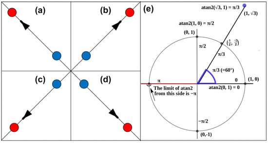
Figure 6.
Red circle shows moving object’s noisy position, blue circle shows the current weighted mean of the particle filter (PF), and arrows show the direction of moving object relative to the current weighted mean of the PF.
The following simulation results show the performance of the location-based method, for moving object heading estimation from the noisy location information provided by the Real-Time Location System (RTLS). The estimated heading information is used for improving PF’s localization and tracking performance. In Figure 7e the black line shows the pattern of noise added to the location () of the robot, the blue line shows the PF Estimated Position (PFEP), the red line shows the Moving Object Real Position(MORP) and the green line shows the angular noise added. The pattern of noise added in MORP is in accordance with the RTLS noise pattern observed experimentally, described in Figure 1. Angular noise in Figure 7b was added in the original commanded angle of Wheeled Mobile Robot (WMR). WMR was supposed to move along a diagonal path from (0, 0) to (0, 500) by making 45° angle with X-axis. But as shown in Figure 7a,c, because of the angular noise added, the WMR follow a curved path instead of a diagonal path and deviates from its original path shown by the red line. As shown by the blue line in Figure 7c, the PFEP is very close to the real location of the WMR, although the angle was estimated from the noisy location information provided by the RTLS. Zoom in portions of Figure 7c,e are shown in Figure 7d,f. The angular and distance noise effect on the PF localization and tracking performance, and the above two angular error mitigation models (RL and LHE) results are summarized in the Table 1.
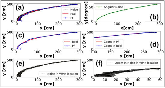
Figure 7.
(a) A comparative picture of moving object’s real position (MORP) and particle filter estimated position (PFEP). (b) Cumulative angular noise versus distance. (c) A clear picture of MORP with noise and PFEP. A zoomed-in portion of (c) is shown in (d). (e) The noise added in MORP, a zoomed-in a portion of which is shown in (f).

Table 1.
Comparison of distance and angular noise effects on particle filter (PF) performance. PF performance enhancement using Reinforcement Learning (RL) and a Location-based Heading Estimation (LHE) for angular noise mitigation.
Table 1, summarize the angular and distance noise effect on PF localization performance presented in Figure 5 and Figure 7. Table 1 shows that our proposed Reinforcement Learning (RL) and Location-based heading estimation methods successfully mitigate the localization error induced by the angular noise. The left column of Table 1 shows the angular noise impact on the Particle Filter (PF) performance while the right column shows distance noise impact on the PF localization performance. Simulation results show that distance uncertainties have minimal impact on PF localization performance while angular uncertainties have an exponential impact on PF localization performance. In the first row of the left column when there is no angular noise, the average localization error is 9.93 cm. A 0.1° angular error was induced in each motion step of the Wheeled Mobile Robot(WMR), which keeps on accumulating up to 54.6°, this angular noise-induced localization error of 98.41 cm in the PF location estimation shown in the second row of left column. The last two rows of left column show that location error induced by the cumulative angular noise was significantly reduced by applying RL and LHE methods for heading estimation. Simulation results show that the proposed heading estimation methods significantly enhance the PF localization and tracking performance in the environment and conditions which results in robot wheel slip.
4.5. RL and LHE Heading Estimation in Large Dimensions
As discussed above that although Deep Q-Network (DQN) based model was trained for 500 cm space it can be applied to any dimensional space by scaling of -coordinates. Similarly, the Location-based Heading Estimation (LHE) can also be applied to any dimensional space without scaling. In Figure 8, both methods were applied for estimating heading of Wheeled Mobile Robot (WMR) in the presence of angular noise. A 1000 cm space was chosen for simulation, 0.1° of angular noise was added in the WMR heading at each motion step, the angular noise was accumulated which induced a large error in PF location estimation. In Figure 8, the black lines show paths followed by the WMR, while green lines show PF location estimation. In Figure 8a,a1, there is zero angular noise in robot heading, and hence the PF localization has a strong correlation with the original path followed by the WMR. In Figure 8b,c, 0.1° of angular noise was added in WMR’s heading at each step of motion, because of the accumulated angular noise the PF localization performance was severely degraded which is shown by the green lines. Figure 8d,d1, shows that when the Reinforcement Learning (RL) based heading estimation was used, PF location estimation (green line) shows a strong correlation with the original path (black line) followed by the WMR. Similarly, when LHE was applied for heading estimation in the presence of angular noise, the PF estimated location (green line) has a strong correlation with the original path (black line) of WMR. Simulation results show that the WMR wheel slip which is caused by the angular noise can be incorporated into localization by using our proposed heading estimation methods. Then the PF localization and desired path information can be used to estimate and compensate the WMR lateral slip.
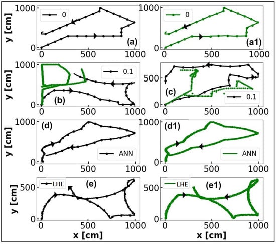
Figure 8.
Black lines show original path followed by a wheeled mobile robot (WMR); green lines show the particle filter (PF) location estimation. (a,a1) Zero angular noise. (b,c) Green lines show PF location estimation of the paths followed by WMR in the presence of cumulative angular noise. (d1,e1) Shows PF location estimation of the paths in (d,e) followed by WMR through the application of reinforcement learning (RL) and Location-based Heading Estimation (LHE) in the presence of angular noise.
4.6. Location-Based Slip Estimation and Compensation
In the above expressions () is a point on the desired path while () is a point on the last index of PF estimation array. WMR is below the desired path if , and above the desired path if . A simple case of the desired path (Figure 9a, redline) is considered for the sake of demonstrating the slip estimation algorithm, although this algorithm can be applied to any linear and non-linear two-dimensional motion. Because of the angular noise, WMR tends to move above the desired path in Figure 9a, and hence for each PF location estimation (, ) of the WMR, the condition of is satisfied for this scenario. Once the value of n is known, then the following formulas are used to find the nearest point on the desired path to the current PF location estimation (, ) of the WMR.
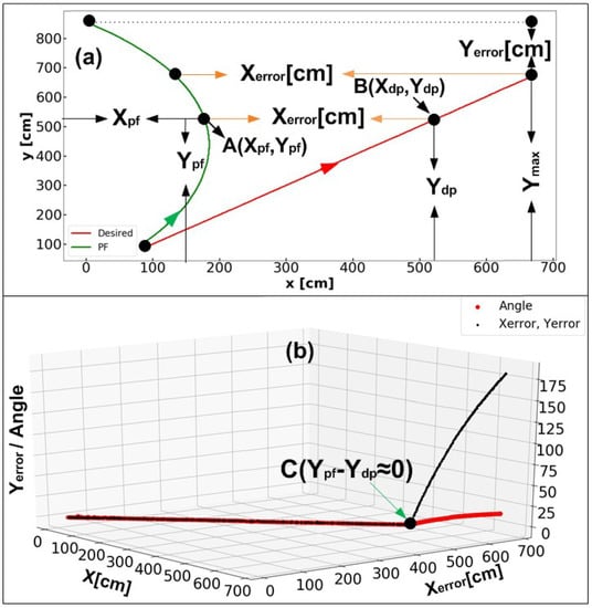
Figure 9.
(a) Green line is the particle filter (PF) location estimation of the wheeled mobile robot (WMR), and red line shows the desired path. (b) The X-axis is similar to the X-axis of (a); and are the WMR’s slip from the desired path along X- and Y-axes, respectively. The red line shows the absolute value of the angle the WMR should move with to return back along the desired path.
In the above formulas, are arrays of the Y- and X-coordinates of the desired path respectively. “abs” mean absolute value, “argmin” will return index of the value in the or which has minimum diffrence with the or respectively. The formulas return index () of the nearest Y-coordinate of if and index () of the nearest X-coordinate of if . As shows in Figure 9a, the nearest Y-coordinate of the PF location estimation at A (, ) is the Y-coordinate () of the point B (, ) on the desired path. Figure 9a shows that the difference ≈ 0 for points A and B, while = is a positive value. For the case of and = the following expression calculate the deviation from the desired path along X- and Y-axis for the WMR’s current PF estimated location (, ).
In the above expression is maximum Y-coordinates of the desired path represented by the in Figure 9a. For the second case when n = 0 and = the following expression calculate the deviation of WMR from the desired path along X- and Y-axis.
In the above 2 expressions , are deviations of WMR from the desired path along X- and Y-axis. Furthermore, is used to find the direction along which the robot has to move along to get back to the desired path and compensate the wheel slip caused by the angular noise. As shown by the black line in Figure 9b, that lateral slip deviation (), is almost zero till C(≈ 0), after point C, along with , also increases. Redline in Figure 9b shows the angle of the direction that WMR should move along to get back to the desired path. For the situation of Figure 9a, the angle values are either zero or negative but only their absolute values are shown by the red line in Figure 9b, so 15°° in the clockwise direction or +345° in the anticlockwise direction. Redline in Figure 9b shows the angle that WMR should move with to get back along the desired path is zero until point C, and then its value decreases to reach −15. A map of the is provided in Figure 6e.
The above lateral wheels slip estimation method is simple to implement, it is robust and computationally not expensive. This WMR’s wheels slip estimation can be applied to a robot with any numbers of wheels and robot of any shape. This method is applicable both in the indoor and outdoor environment. The method can include the measurement uncertainty of sensors used for slip estimation. It can be applied to both linear and non-linear problems. It can be implemented to estimate wheel slip of a robot moving on any type of terrain. Table 2 shows that our proposed method outperforms many state of the art methods in many aspects.
Table 2.
Methods and approaches adopted for vehicle sideslip angle (VSA) estimation. SMO: sliding-mode observer; KF: Kalman filter; EKF extended Kalman filter; CS: current sensing; IS: inertial sensors; RL & LHE: reinforcement learning & Location-based Heading Estimation.
5. Conclusions
An attempt is made to quantify the distance and angular noise effect on the performance of PF. The results show the minimal effect of distance noise while the exponential effect of angular noise on the PF performance. Reinforcement Learning (RL) and Location-based Heading Estimation (LHE) are proposed for mitigating angular noise effect on Particle Filter (PF) localization performance, in a drift-prone environment. Heading of the Wheeled Mobile Robot (WMR) was estimated from the noisy location information provided by the Real-Time Location System (RTLS) using trilateration, and the current weighted mean of the PF by using RL and LHE. The estimated heading was then used to improve the localization performance of the PF in the presence of angular noise. By using the proposed solutions, angular noise caused by the slip can be implicitly incorporated into the PF location estimation. This is a very robust algorithm for the environment with robot wheel slip on a slippery or sandy ground, and a robot with noisy steering systems. The algorithm can incorporate both linear and non-linear angular noise of any magnitude. Furthermore, an algorithm is proposed for WMR’s wheel slip estimation and compensation by using the desired path information and PF location estimation. A DecaWave based ranging system is proposed, which benefits from the advantages of UWB radio communication, such as low power consumption, robustness in the multipath padding environments, and long-ranging. This ranging system is a good solution for resources-constrained robots in the indoor environment. Simulation results show that the PF localization performance in the presence of angular noise that results from the WMR’s wheels slip is significantly improved by application of the above two methods. Simulation results also show that wheel lateral slip can be accurately estimated from the PF location estimation and desired path information. Lateral slip information can be used to make decisions for moving WMR back toward the desired path.
Author Contributions
Z.U. developed the main idea, which was discussed with all the authors; Z.L. and Z.X. guide and support me in implementing the idea; Z.U. executed and implemented the idea and report the results; Z.X. and L.Z. help to review and improve the paper.
Acknowledgments
The authors would like to thank, CAS-TWAS President’s Ph.D. Fellowship Programme, University of Chinese Academy of Sciences and Innovation Project of Institute of Computing Technology, Chinese Academy of Sciences, for supporting this research work. The author would also like to thank the anonymous reviewers for their valuable comments and suggestions.
Conflicts of Interest
The authors declare no conflict of interest.
References
- Iossaqui, J.G.; Camino, J.F. Wheeled Robot Slip Compensation for Trajectory Tracking Control Problem with Time-Varying Reference Input. In Proceedings of the 9th International Workshop on Robot Motion and Control, Nagoya, Japan, 3–5 July 2013; pp. 167–173. [Google Scholar]
- He, W.; Dong, Y.; Sun, C. Adaptive Neural Impedance Control of a Robotic Manipulator With Input Saturation. IEEE Trans. Syst. Man Cybern. Syst. 2016, 46, 334–344. [Google Scholar] [CrossRef]
- Tian, Y.; Sarkar, N. Control of a Mobile Robot Subject to Wheel Slip. J. Intell. Robot. Syst. 2013, 74, 915–929. [Google Scholar] [CrossRef]
- Chindamo, D.; Lenzo, B.; Gadola, M. On the Vehicle Sideslip Angle Estimation: A Literature Review of Methods, Models, and Innovations. Appl. Sci. 2018, 8, 355. [Google Scholar] [CrossRef]
- Yamauchi, G.; Suzuki, D.; Nagatani, K. Online Slip Parameter Estimation for Tracked Vehicle Odometry on Loose Slope. In Proceedings of the IEEE International Symposium on Safety, Security, and Rescue Robotics (SSRR), Lausanne, Switzerland, 23–27 October 2016; pp. 227–232. [Google Scholar]
- D’Vidhyaprakash, A.E. Studies on Affecting Factors of Wheel Slip and Odometry Error on Real-Time of Wheeled Mobile Robots: A Review. Studies 2016, 1130. [Google Scholar] [CrossRef]
- Sidharthan, R.K.; Kannan, R.; Srinivasan, S.; Balas, V.E. Stochastic Wheel-Slip Compensation Based Robot Localization and Mapping. Adv. Electr. Comp. Eng. 2016, 16, 25–32. [Google Scholar] [CrossRef]
- Yi, J.; Zhang, J.; Song, D.; Jayasuriya, S. IMU-based Localization and Slip Estimation for Skid-Steered Mobile Robots. In Proceedings of the IEEE/RSJ International Conference on Intelligent Robots and Systems, San Diego, CA, USA, 29 October–2 November 2007; pp. 2845–2850. [Google Scholar]
- Ojeda, L.; Cruz, D.; Reina, G.; Borenstein, J. Current-Based Slippage Detection and Odometry Correction for Mobile Robots and Planetary Rovers. IEEE Trans. Robot. 2006, 22, 366–378. [Google Scholar] [CrossRef]
- Kim, D.E.; Yoon, H.N.; Kim, K.S.; Sreejith, M.; Lee, J.M. Using Current Sensing Method and Fuzzy PID Controller for Slip Phenomena Estimation and Compensation of Mobile Robot. In Proceedings of the 14th International Conference on Ubiquitous Robots and Ambient Intelligence (URAI), Jeju, Korea, 28 June–1 July 2017; pp. 397–401. [Google Scholar]
- Partovibakhsh, M.; Liu, G. Slip Ratio Estimation and Control of Wheeled Mobile Robot on Different Terrains. In Proceedings of the IEEE International Conference on Cyber Technology in Automation, Control, and Intelligent Systems (CYBER), Shenyang, China, 8–12 June 2015; pp. 566–571. [Google Scholar]
- Berntorp, K. Particle Filter for Combined Wheel-Slip and Vehicle-Motion Estimation. In Proceedings of the American Control Conference (ACC), Chicago, IL, USA, 1–3 July 2015; pp. 5414–5419. [Google Scholar]
- Reina, G.; Ishigami, G.; Nagatani, K.; Yoshida, K. Vision-Based Estimation of Slip Angle for Mobile Robots and Planetary Rovers. In Proceedings of the IEEE International Conference on Robotics and Automation, Nice, France, 22–26 September 2008; pp. 486–491. [Google Scholar]
- Patil, M.; Abukhalil, T.; Sobh, T.S. Hardware Architecture Review of Swarm Robotics System: Self-Reconfigurability, Self-Reassembly, and Self-Replication. In Innovations and Advances in Computing, Informatics, Systems Sciences, Networking and Engineering; Springer: Cham, Switzerland, 2015. [Google Scholar]
- Patil, M.; Abukhalil, T.; Patel, S.; Sobh, T. UB Robot Swarm-Design, Implementation, and Power Management. In Proceedings of the 12th IEEE International Conference on Control and Automation (ICCA), Kathmandu, Nepal, 1–3 June 2016; pp. 577–582. [Google Scholar]
- Li, F.; Zhao, C.; Ding, G.; Gong, J.; Liu, C.; Zhao, F. A Reliable and Accurate Indoor Localization Method Using Phone Inertial Sensors. In Proceedings of the ACM Conference on Ubiquitous Computing, Pittsburgh, PA, USA, 5–8 September 2012; pp. 421–430. [Google Scholar]
- Choi, K.H.; Ra, W.S.; Park, S.Y.; Park, J.B. Robust Least Squares Approach to Passive Target Localization Using Ultrasonic Receiver Array. IEEE Trans. Ind. Electron. 2014, 61, 1993–2002. [Google Scholar] [CrossRef]
- Kim, S.J.; Kim, B.K. Dynamic Ultrasonic Hybrid Localization System for Indoor Mobile Robots. IEEE Trans. Ind. Electron. 2013, 60, 4562–4573. [Google Scholar] [CrossRef]
- Saab, S.S.; Nakad, Z.S. A Standalone RFID Indoor Positioning System Using Passive Tags. IEEE Trans. Ind. Electron. 2011, 58, 1961–1970. [Google Scholar] [CrossRef]
- Yang, P.; Wu, W. Efficient Particle Filter Localization Algorithm in Dense Passive RFID Tag Environment. IEEE Trans. Ind. Electron. 2014, 61, 5641–5651. [Google Scholar] [CrossRef]
- Yang, P.; Wu, W.; Moniri, M.; Chibelushi, C.C. Efficient Object Localization Using Sparsely Distributed Passive RFID Tags. IEEE Trans. Ind. Electron. 2013, 60, 5914–5924. [Google Scholar] [CrossRef]
- Yoon, S.; Lee, K.; Rhee, I. FM-based Indoor Localization via Automatic Fingerprint DB Construction and Matching. In Proceedings of the 11th Annual International Conference on Mobile Systems, Applications, and Services, Taipei, Taiwan, 25–28 June 2013; pp. 207–220. [Google Scholar]
- Chung, J.; Donahoe, M.; Schmandt, C.; Kim, I.J.; Razavi, P.; Wiseman, M. Indoor Location Sensing Using Geo-Magnetism. In Proceedings of the 9th international conference on Mobile Systems, Applications, and Services, Bethesda, MD, USA, 28 June–1 July 2011; pp. 141–154. [Google Scholar]
- Li, B.; Gallagher, T.; Dempster, A.G.; Rizos, C. How Feasible is the Use of Magnetic Field Alone for Indoor Positioning? In Proceedings of the International Conference on Indoor Positioning and Indoor Navigation (IPIN), Sydney, Australia, 13–15 November 2012; pp. 1–9. [Google Scholar]
- Rai, A.; Chintalapudi, K.K.; Padmanabhan, V.N.; Sen, R. Zee: Zero-Effort Crowdsourcing for Indoor Localization. In Proceedings of the 18th Annual International Conference on Mobile Computing and Networking, Istanbul, Turkey, 22–26 August 2012. [Google Scholar]
- Mendes, C. Stereo-Based Autonomous Navigation and Obstacle Avoidance. IFAC Proc. Vol. 2013, 46, 211–216. [Google Scholar] [CrossRef]
- Zhen, W.; Zeng, S.; Soberer, S. Robust Localization and Localizability Estimation with a Rotating Laser Scanner. In Proceedings of the IEEE International Conference on Robotics and Automation (ICRA), Singapore, 29 May–3 June 2017; pp. 6240–6245. [Google Scholar]
- Sharifi, M.; Chen, X. Introducing A Novel Vision Based Obstacle Avoidance Technique for Navigation of Autonomous Mobile Robots. In Proceedings of the IEEE 10th Conference on Industrial Electronics and Applications (ICIEA), Auckland, New Zealand, 15–17 June 2015. [Google Scholar]
- Alwan, M.; Wagner, M.B.; Wasson, G.; Sheth, P. Characterization of Infrared Range-Finder PBS-03JN for 2-D Mapping. In Proceedings of the IEEE International Conference on Robotics and Automation, Barcelona, Spain, 18–22 April 2005; pp. 3936–3941. [Google Scholar]
- Jimenez, J.A.; Urena, J.; Mazo, M.; Hernandez, A.; Santiso, E. Three-Dimensional Discrimination between Planes, Corners and Edges Using Ultrasonic Sensors. In Proceedings of the IEEE Conference on Emerging Technologies and Factory Automation, Lisbon, Portugal, 16–19 September 2003; Volume 2, pp. 692–699. [Google Scholar]
- Memon, K.R.; Memon, S.; Memon, B.; Memon, A.R.; Shah, S.M.Z.A. Real Time Implementation of Path Planning Algorithm with Obstacle Avoidance for Autonomous Vehicle. In Proceedings of the 3rd International Conference on Computing for Sustainable Global Development (INDIACom), New Delhi, India, 16–18 March 2016; pp. 2048–2053. [Google Scholar]
- Ortiz, G.; Treven, F.; Svensson, L.; Larsson-Edefors, P.; Johansson-Mauricio, S. A Framework for a Relative Real-Time Tracking System based on Ultra-Wideband Technology. In Proceedings of the 14th Workshop on Positioning, Navigation and Communications (WPNC), Berlin/Heidelberg, Germany, 25–26 October 2017; pp. 1–6. [Google Scholar]
- Meissner, P.; Leitinger, E.; Witrisal, K. UWB for Robust Indoor Tracking: Weighting of Multipath Components for Efficient Estimation. IEEE Wirel. Commun. Lett. 2014, 3, 501–504. [Google Scholar] [CrossRef]
- Fox, D.; Hightower, J.; Kauz, H.; Liao, L.; Patterson, D. Bayesian Techniques for Location Estimation. In Proceedings of the Workshop on Location-Aware Computing, Orlando, FL, USA, 4 December 2003. [Google Scholar]
- Savic, V.; Larsson, E.G. Experimental Study of Indoor Tracking Using UWB Measurements and Particle Filtering. In Proceedings of the IEEE 17th International Workshop on Signal Processing Advances in Wireless Communications (SPAWC), Edinburgh, UK, 3–6 July 2016; pp. 1–5. [Google Scholar]
- Su, Y.; Zhao, Q.; Zhao, L.; Gu, D. Abrupt motion tracking using a visual saliency embedded particle filter. Patt. Recognit. 2014, 47, 1826–1834. [Google Scholar] [CrossRef]
- Gustafsson, F.; Gunnarsson, F.; Bergman, N.; Forssell, U.; Jansson, J.; Karlsson, R.; Nordlund, P.J. Particle filters for positioning, navigation, and tracking. IEEE Trans. Signal Proc. 2002, 50, 425–437. [Google Scholar] [CrossRef]
- Arulampalam, M.S.; Maskell, S.; Gordon, N.; Clapp, T. A tutorial on particle filters for online nonlinear/non-Gaussian Bayesian tracking. IEEE Trans. Signal Proc. 2002, 50, 174–188. [Google Scholar] [CrossRef]
- Park, D.H.; Stephanie, S.; Porter, R.L. Sensitivity to Noise in Particle Filters for 2-D Tracking Algorithms. Nursing 2013, 6, 58–65. [Google Scholar]
- McElroy, C.; Neirynck, D.; McLaughlin, M. Comparison of Wireless Clock Synchronization Algorithms for Indoor Location Systems. In Proceedings of the IEEE International Conference on Communications Workshops (ICC), Sydney, Australia, 10–14 June 2014; pp. 157–162. [Google Scholar]
- Ye, T.; Walsh, M.; Haigh, P.; Barton, J.; O’Flynn, B. Experimental Impulse Radio IEEE 802.15.4a UWB based Wireless Sensor Localization Technology: Characterization, Reliability and Ranging. In Proceedings of the 22nd IET Irish Signals and Systems Conference, Dublin, Ireland, 23–24 June 2011. [Google Scholar]
© 2018 by the authors. Licensee MDPI, Basel, Switzerland. This article is an open access article distributed under the terms and conditions of the Creative Commons Attribution (CC BY) license (http://creativecommons.org/licenses/by/4.0/).