Normal Bases on Galois Ring Extensions

Abstract

Normal bases are widely used in applications of Galois fields and Galois rings in areas such as coding, encryption symmetric algorithms (block cipher), signal processing, and so on. In this paper, we study the normal bases for Galois ring extension $\mathbf{R}/{\mathrm{Z}}_{p^r}$, where $\mathbf{R}=\mathrm{GR}(p^r,n).$ We present a criterion on the normal basis for $\mathbf{R}/{\mathrm{Z}}_{p^r}$ and reduce this problem to one of finite field extension $\overline{\mathbf{R}}/{\overline{\mathrm{Z}}}_{p^r}={\mathbb{F}}_q/{\mathbb{F}}_p(q=p^n)$ by Theorem 1. We determine all optimal normal bases for Galois ring extension.

1. Introduction

The theory of finite fields has been one of the fundamental mathematical tools in computer science and communication engineering since the 1950s, when digit communications and computations were rapidly developed. Low complexity operation, particularly the multiplicative operation, squaring, and exponentiation operations, are preferred in various applications, including coding, cryptography, and communication. The performance of these operations is closely related to the representation of the finite elements; they are desired for efficient hardware implementation, and in this respect, many useful bases for ${\mathbb{F}}_{q^n}/{\mathbb{F}}_q$ with low complexity have been found [1,2,3,4,5,6,7,8,9,10,11]. An efficient algorithm for field multiplication using a normal basis was proposed by Massey and Omura in 1985 [12].

In the past two decades, Galois rings have been used successfully in many aspects, such as in combinatorics to construct different kinds of combinatorial designs and in communication theory to construct error-correcting codes, sequences with good correlation properties, secret sharing schemes, hash functions, and so on [3,13,14,15,16]. However, compared to the case of finite field extensions, the complexity problem of operations in Galois rings has not attracted much attention from scholars, except Abrahamsson, who considered the complexity of bases and carefully discussed the architectures for multiplication in Galois rings (for $p=2$) in his thesis [17] in 2004. These are motivation by our study of operations, particularly for multiplicative operation, with low complexity in Galois rings.

In this paper, we study one aspect of the complexity problem of operations in Galois rings. More precisely, we mainly focus on the normal bases for Galois ring extensions. This paper is organized as follows. In Section 2, we introduce some basic facts on Galois rings. Some results on normal bases and some basic properties on the multiplicative complexity of normal bases for Galois ring extension $\mathrm{GR}(p^r,n)/{\mathrm{Z}}_{p^r}$ are presented in Section 3. Then, we determine all optimal normal bases for these Galois ring extensions in Section 4.

2. Basic Facts about Galois Rings

In this section, we introduce several basic facts about Galois rings. For more information, the reader is referred to [18].

Let p be a prime number and $r\ge 2,{\mathrm{Z}}_{p^r}=\mathbb{Z}/p^r\mathbb{Z}.$ We have the modulo p reduction mapping:

$$\phi :{\mathrm{Z}}_{p^r}⟶{\mathbb{F}}_p,a(mod{p}^r)⟼\overline{a}=a(modp),$$

which induces the following modulo p reduction mapping between polynomial rings:

$$\phi :{\mathrm{Z}}_{p^r}[x]⟶{\mathbb{F}}_p[x],f(x)=\sum c_i{x}^i⟼\overline{f}(x)=\sum {\overline{c}}_i{x}^i.$$

$f(x)$ is said to be a monic basic irreducible (primitive) polynomial over ${\mathrm{Z}}_{p^r}$ if $\overline{f}(x)$ is a monic irreducible (primitive) polynomial over ${\mathbb{F}}_p.$

Let $f(x)$ be a basic primitive polynomial of degree n in ${\mathrm{Z}}_{p^r}[x].$ The quotient ring:

$$\begin{array}{ccc}\hfill \mathbf{R}& =& \mathrm{GR}(p^r,n)=\frac{{\mathrm{Z}}_{p^r}[x]}{(f(x))}\cong {\mathrm{Z}}_{p^r}[\gamma ]\hfill \\ & =& \{c_0+c_1\gamma +\cdots +c_{n-1}{\gamma }^{n-1}:c_i\in {\mathrm{Z}}_{p^r}\},\hfill \end{array}$$

(1)

where $\gamma$ is a root of $f(x)$ in $\mathbf{R}$ with order $p^n-1$, $\mathbf{R}$ is called a Galois ring. We note that $\overline{\gamma }$ is a primitive element of the finite field ${\mathbb{F}}_q$ where $q=p^n.$ From now on, we take $f(x)$ to be a basic primitive polynomial. The modulo p reduction can be naturally extended to the following homomorphism of rings:

$$\phi :\mathbf{R}=\mathrm{GR}(p^r,n)=\frac{{\mathrm{Z}}_{p^r}[x]}{(f(x))}\cong {\mathrm{Z}}_{p^r}[\gamma ]⟶{\mathbb{F}}_q=\frac{{\mathbb{F}}_p[x]}{(\overline{f}(x))}\cong {\mathbb{F}}_p[\overline{\gamma }].$$

Some basic facts about Galois ring $\mathbf{R}=\mathrm{GR}(p^r,n)$ are given as follows.

(Fact 1) Let ${\mathrm{T}}^{*}=\langle \gamma \rangle$ be the cyclic multiplicative group of order $q-1$ generated by $\gamma$, and $\mathrm{T}={\mathrm{T}}^{*}\cup \{0\}.$ Then, $\overline{\mathrm{T}}={\mathbb{F}}_q$ and:

$$\mathbf{R}=\{x_0+p{x}_1+p^2{x}_2+\cdots +p^{r-1}{x}_{r-1}:x_i\in \mathrm{T}\},\left|\mathbf{R}\right|={\left|\mathrm{T}\right|}^r=q^r=p^{nr}.$$

(2)

(Fact 2) $\mathbf{R}$ is a local commutative ring with the unique maximal ideal $\mathcal{M}=p\mathbf{R},\left|\mathcal{M}\right|=q^{r-1}$, and the group of units is ${\mathbf{R}}^{*}=\mathbf{R}\backslash \mathcal{M}={\mathrm{T}}^{*}\times (1+\mathcal{M}),\left|{\mathbf{R}}^{*}\right|=q^r-q^{r-1}.$

(Fact 3) $\mathbf{R}/{\mathrm{Z}}_{p^r}$ is a Galois extension of rings with Galois group $Gal(\mathbf{R}/{\mathrm{Z}}_{p^r})=\langle {\sigma }_p\rangle ,$ where ${\sigma }_p$ is the automorphism of order n defined by:

$${\sigma }_p(\sum _{i=0}^{r-1}{p}^i{x}_i)=\sum _{i=0}^{r-1}{p}^i{x}_i^p(x_i\in \mathrm{T}).$$

(3)

More generally, for each positive integer $l,\mathbf{R}=\mathrm{GR}(p^r,n)$ is a subring of ${\mathbf{R}}_{(l)}=\mathrm{GR}(p^r,nl)$ and ${\mathbf{R}}_{(l)}/\mathbf{R}$ is a Galois extension of rings with Galois group $Gal({\mathbf{R}}_{(l)}/\mathbf{R})=\langle {\sigma }_q\rangle ,$ where ${\sigma }_q$ is the automorphism of ${\mathbf{R}}_{(l)}$ defined by:

$${\sigma }_q(\sum _{i=0}^{r-1}{p}^i{x}_i)=\sum _{i=0}^{r-1}{p}^i{x}_i^q(x_i\in {\mathrm{T}}_{(l)}),$$

(4)

and ${\mathbf{R}}_{(l)}={\mathrm{Z}}_{p^r}[{\gamma }_{(l)}]=\{{\sum }_{i=0}^{r-1}{p}^i{x}_i:x_i\in {\mathrm{T}}_{(l)}\},{\mathrm{T}}_{(l)}={\mathrm{T}}_{(l)}^{*}\cup \{0\},{\mathrm{T}}_{(l)}^{*}=\langle {\gamma }_{(l)}\rangle ,{\gamma }_{(l)}^{\frac{q^l-1}{q-1}}=\gamma .$

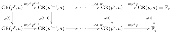
(Fact 4) We have the trace mapping:

$${\mathrm{Tr}}_n^{nl}:{\mathbf{R}}_{(l)}=\mathrm{GR}(p^r,nl)⟶\mathbf{R}=\mathrm{GR}(p^r,n),$$

defined by:

$${\mathrm{Tr}}_n^{nl}(\alpha )=\sum _{i=0}^{l-1}{\sigma }_q^i(\alpha )(\alpha \in {\mathbf{R}}_{(l)}),$$

which is an epimorphism of $\mathbf{R}$-modules, and we have the following commutative diagram:

(5)

where ${\mathrm{tr}}_n^{nl}$ and ${\mathrm{tr}}_1^n$ are the trace mappings for finite field extensions.

On the other hand, for $r\ge 2,$ the modulo $p^{r-1}$ reduction gives the homomorphism of rings $\mathrm{GR}(p^r,n)⟶\mathrm{GR}(p^{r-1},n)$, and we get the following commutative diagram:

(6)

where ${\sigma }^{(\lambda )}$ is the automorphism of $\mathrm{GR}(p^{\lambda },n)$ defined by:

$${\sigma }^{(\lambda )}(\sum _{i=0}^{\lambda -1}{p}^i{x}_i)=\sum _{i=0}^{\lambda -1}{p}^i{x}_i^p(x_i\in \mathrm{T}).$$

Next, we need some basic properties of the polynomial ring $\mathbf{R}[x].$ One of the most important properties of $\mathbf{R}[x]$ is the following Hensel’s lemma.

Two polynomials $f(x)$ and $g(x)$ in $\mathbf{R}[x]$ are called coprime if there exist $A(x)$ and $B(x)$ in $\mathbf{R}[x]$ such that $f(x)A(x)+g(x)B(x)=1.$

Lemma 1.

([18], Lemma 14.20) Let $\mathbf{R}=\mathrm{GR}(p^r,n)$ and $\overline{\mathbf{R}}={\mathbb{F}}_q(q=p^n).$ Let $f(x)$ be a monic polynomial in $\mathbf{R}[x]$ and $g_i(x)(1\le i\le s)$ be pairwise coprime monic polynomials in $\overline{\mathbf{R}}[x].$ If $\overline{f}(x)=g_1(x)g_2(x)\cdots g_s(x)$ in $\overline{\mathbf{R}}[x],$ then there exist pairwise coprime polynomials $f_i(x)(1\le i\le s)$ in $\mathbf{R}[x]$ such that $f(x)=f_1(x)f_2(x)\cdots f_s(x)$ and ${\overline{f}}_i(x)=g_i(x)(1\le i\le s).$

The polynomial $f_i(x)$ is called the Hensel lift of $g_i(x).$ A monic polynomial $f(x)$ in $\mathbf{R}[x]$ is called primary if $\overline{f}(x)$ is a power of a monic irreducible polynomial in ${\mathbb{F}}_q[x]$. One can deduce the following result from the Hensel’s lemma.

Lemma 2.

([18], Theorem 14.21) Let $f(x)$ be a monic polynomial of $degf\ge 1$ in $\mathbf{R}[x].$ We have the following decomposition:

$$f(x)=f_1(x)f_2(x)\cdots f_r(x),$$

where $f_i(x)(1\le i\le r)$ are pairwise coprime primary polynomials in $\mathbf{R}[x]$ and $f_i(x)(1\le i\le r)$ are uniquely determined up to their order. Particularly, if $\overline{f}(x)=p_1(x)p_2(x)\cdots p_r(x)$ where $p_i(x)(1\le i\le r)$ are distinct monic irreducible polynomials in $\overline{\mathbf{R}}[x]={\mathbb{F}}_q[x],$ then $f_i(x)(1\le i\le r)$ are distinct monic irreducible polynomials in $\mathbf{R}[x]$ and ${\overline{f}}_i(x)=p_i(x)(1\le i\le r).$

3. Criteria on Normal Bases for Galois Ring Extensions

From (1), we know that $\mathbf{R}=\mathrm{GR}(p^r,n)$ is a free ${\mathrm{Z}}_{p^r}$-module of rank n and $\{1,\gamma ,\cdots ,{\gamma }^{n-1}\}$ is a basis for $\mathbf{R}/{\mathrm{Z}}_{p^r}$, where $\gamma$ is an element of order $q-1(q=p^n)$ in $\mathbf{R}.$

Definition 1.

An element $\alpha \in \mathbf{R}$ is called a normal basis generator (NBG) for extension $\mathbf{R}/{\mathrm{Z}}_{p^r}$ if $\mathfrak{B}=\{{\sigma }^0(\alpha )=\alpha ,\sigma (\alpha ),\cdots ,{\sigma }^{n-1}(\alpha )\}$ is a basis for $\mathbf{R}/{\mathrm{Z}}_{p^r}$, where σ is the automorphism ${\sigma }_p$ of $\mathbf{R}$ defined by (3). Such a basis $\mathfrak{B}$ is called a normal basis for $\mathbf{R}/{\mathrm{Z}}_{p^r}$.

In this section, we present several criteria on normal bases for Galois ring extension $\mathbf{R}/{\mathrm{Z}}_{p^r}$, and these criteria can be reduced to the ones of finite field extensions $\overline{\mathbf{R}}/{\overline{\mathrm{Z}}}_{p^r}={\mathbb{F}}_q/{\mathbb{F}}_p$ according to the following theorem. Recall that an element $a\in {\mathbb{F}}_q(q=p^n)$ is an NBG for ${\mathbb{F}}_q/{\mathbb{F}}_p$ if $\mathfrak{B}=\{a,\overline{\sigma }(a),\cdots ,{\overline{\sigma }}^{n-1}(a)\}$ is a normal basis for ${\mathbb{F}}_q/{\mathbb{F}}_p,$ where $\overline{\sigma }$ is the Frobenius automorphism of ${\mathbb{F}}_q$ defined by $\overline{\sigma }(b)=b^p$ for $b\in {\mathbb{F}}_q.$ From the definition of $\sigma$ in (3), one has for $\alpha \in \mathbf{R},\overline{\sigma (\alpha )}=\overline{\sigma }(\overline{\alpha }).$

Theorem 1.

For an element α in $\mathbf{R}$, α is an NBG for $\mathbf{R}/{\mathrm{Z}}_{p^r}$ if and only if $\overline{\alpha }$ is an NBG for finite field extension $\overline{\mathbf{R}}/{\overline{\mathrm{Z}}}_{p^r}={\mathbb{F}}_q/{\mathbb{F}}_p.$

Proof. 

Suppose that $\overline{\alpha }$ is not an NBG for ${\mathbb{F}}_q/{\mathbb{F}}_p.$ Then, there exist $a_i\in {\mathbb{F}}_p(0\le i\le n-1)$ such that:

$$\sum _{i=0}^{n-1}{a}_i{\overline{\sigma }}^i(\overline{\alpha })=0$$

(7)

and $a_j\ne 0$ for some $j.$ Let $A_i\in \mathbf{R},\overline{A_i}=a_i(0\le i\le n-1).$ The formula (7) implies that $\overline{{\sum }_{i=0}^{n-1}{A}_i{\sigma }^i(\alpha )}={\sum }_{i=0}^{n-1}{a}_i{\overline{\sigma }}^i(\overline{\alpha })=0$, so that ${\displaystyle \sum _{i=0}^{n-1}}{A}_i{\sigma }^i(\alpha )\in p\mathbf{R}.$ Therefore, ${\displaystyle \sum _{i=0}^{n-1}}{p}^{r-1}{A}_i{\sigma }^i(\alpha )=0.$ From $a_j\in {\mathbb{F}}_p^{\times }$, we know that $A_j\in {\mathbf{R}}^{*}$ and $p^{r-1}{A}_j\ne 0.$ Therefore, $\alpha$ is not an NBG for $\mathbf{R}/{\mathrm{Z}}_{p^r}$.

On the other hand, suppose that $\alpha$ is not an NBG for $\mathbf{R}/{\mathrm{Z}}_{p^r}.$ Then, there exist $A_i\in \mathbf{R}(0\le i\le n-1)$ such that:

$$\sum _{i=0}^{n-1}{A}_i{\sigma }^i(\alpha )=0$$

(8)

and $A_j\ne 0$ for some $j.$ Let $A_i\in p^{d_i}\mathbf{R}\backslash p^{d_i+1}\mathbf{R}(0\le i\le n-1)$ and $d=min\{d_i|0\le i\le n-1\}.$ From $A_j\ne 0$, we get $0\le d\le r-1.$ Then, $A_i=p^d{a}_i$, where $a_i\in \mathbf{R}(0\le i\le n-1)$ and $a_j\in {\mathbf{R}}^{*}$ by assuming $A_j\in p^d\mathbf{R}\backslash p^{d+1}\mathbf{R}$. The formula (8) implies that $p^d{\displaystyle \sum _{i=0}^{n-1}}{a}_i{\sigma }^i(\alpha )=0$, so that ${\displaystyle \sum _{i=0}^{n-1}}{a}_i{\sigma }^i(\alpha )\in p^{r-d}\mathbf{R}.$ Then, from $r-d\ge 1$, we get ${\displaystyle \sum _{i=0}^{n-1}}{\overline{a}}_i{\overline{\sigma }}^i(\overline{\alpha })=0$, where ${\overline{a}}_i\in {\mathbb{F}}_p(0\le i\le n-1)$ and ${\overline{a}}_j\ne 0.$ Therefore, $\overline{\alpha }$ is not an NBG for ${\mathbb{F}}_q/{\mathbb{F}}_p.$ This completes the proof of Theorem 1. □

By Theorem 1, a series of criteria on normal bases for finite field extensions can be shifted to ones for Galois ring extensions.

Lemma 3.

([19])Let $n=p^{t}l,(l,p)=1,Q=p^n$ and $q=p^l.$ Let ${\mathrm{tr}}_q^Q$ be the trace mapping for ${\mathbb{F}}_Q/{\mathbb{F}}_q.$ Then, for $a\in {\mathbb{F}}_Q,a$ is an NBG for ${\mathbb{F}}_Q/{\mathbb{F}}_p$ if and only if ${\mathrm{tr}}_q^Q(a)$ is an NBG for ${\mathbb{F}}_q/{\mathbb{F}}_p.$

From the diagram (5), we know that for $\alpha \in \mathbf{R},{\mathrm{tr}}_l^n(\overline{\alpha })=\overline{{\mathrm{Tr}}_l^n(\alpha )}.$

Corollary 1.

Let $n=p^{t}l,(l,p)=1.$ Let $\mathbf{R}=\mathrm{GR}(p^r,n),{\mathbf{R}}^{\prime }=\mathrm{GR}(p^r,l)$, and $\mathrm{Tr}:\mathbf{R}\to {\mathbf{R}}^{\prime }$ be the trace mapping from $\mathbf{R}$ to ${\mathbf{R}}^{\prime }.$ Then, for $\alpha \in \mathbf{R},\alpha$ is an NBG for $\mathbf{R}/{\mathrm{Z}}_{p^r}$ if and only if $\mathrm{Tr}(\alpha )$ is an NBG for ${\mathbf{R}}^{\prime }/{\mathrm{Z}}_{p^r}.$

By Corollary 1, we assume $(n,p)=1$ without loss of generality. In this case, $x^n-1$ has the following decomposition in the polynomial ring ${\mathbb{F}}_p[x]:$

$$x^n-1=p_1(x)p_2(x)\cdots p_r(x),$$

(9)

where $p_1(x),p_2(x),\cdots ,p_r(x)$ are distinct monic irreducible polynomials in ${\mathbb{F}}_p[x].$

Let ${\mathcal{F}}_p[x]$ be the set of all p-polynomials ${\displaystyle \sum _i}{c}_i{x}^{p^i}(c_i\in {\mathbb{F}}_p)$. Then, ${\mathcal{F}}_p[x]$ is a ring with respect to the ordinary addition, and the following multiplication defined by composition ⊗:

$$F(x)\otimes G(x)=F(G(x)),\mathrm{for}F(x),G(x)\in {\mathcal{F}}_p[x],$$

and the mapping:

$$\mu :{\mathbb{F}}_p[x]⟶{\mathcal{F}}_p[x],\sum _i{c}_i{x}^i⟶\sum _i{c}_i{x}^{p^i}$$

is an isomorphism of rings. Corresponding to the decomposition (9) in ${\mathbb{F}}_p[x],$ we have the following decomposition of:

$$x^{p^n}-x=P_1(x)\otimes P_2(x)\otimes \cdots \otimes P_r(x),$$

where $P_i(x)=\mu (p_i(x))(1\le i\le r)$ are distinct monic irreducible p-polynomials in ${\mathcal{F}}_p[x]$. Let $m_i(x)=\frac{x^n-1}{p_i(x)}$ and $M_i(x)=\mu (m_i(x))={\displaystyle \underset{\genfrac{}{}{0pt}{}{\lambda =1}{\lambda \ne i}}{\overset{r}{⨂}}}{P}_{\lambda }(x)\in {\mathcal{F}}_p[x].$

Lemma 4.

([18]) Let $q=p^n$ and $(n,p)=1.$ For $a\in {\mathbb{F}}_q,a$ is an NBG for ${\mathbb{F}}_q/{\mathbb{F}}_p$ if and only if $M_i(a)\ne 0(1\le i\le r)$.

This is a direct consequence of Theorem 1 and Lemma 4. We have the following criterion.

Corollary 2.

Let $\mathbf{R}=\mathrm{GR}(p^r,n)$, where $(n,p)=1.$ Then, for $\alpha \in \mathbf{R},\alpha$ is an NBG for $\mathbf{R}/{\mathrm{Z}}_{p^r}$ if and only if $M_i(\overline{\alpha })\ne 0(1\le i\le r).$

By the decomposition (9), we have:

$$\frac{{\mathbb{F}}_p[x]}{(x^n-1)}=\underset{i=1}{\overset{r}{⨁}}\frac{{\mathbb{F}}_p[x]}{(p_i(x))}\cong \underset{i=1}{\overset{r}{⨁}}{\mathbb{F}}_{p^{d_i}},$$

where $d_i=deg{p}_i(x).$ Then, we have the orthogonal idempotents $e_i(x)\in {\mathbb{F}}_p[x],deg{e}_i(x)\le n-1(1\le i\le r)$ satisfying:

$$e_i(x)\equiv {\delta }_{ij}(mod{p}_j(x))(1\le i\le j\le r),$$

where ${\delta }_{ij}$ is the Kronecker symbol. These idempotents $e_i(x)(1\le i\le r)$ can be computed by using the ${\sigma }_p$-class of the roots of $x^n-1$ (see [19]).

In [19], we present a new criterion of NBG for ${\mathbb{F}}_q/{\mathbb{F}}_p(q=p^n,(n,p)=1)$ by using idempotents in the ring $\frac{{\mathbb{F}}_p[x]}{(x^n-1)}$.

Lemma 5.

([19]) Letting $E_i(x)=\mu (e_i(x))\in {\mathcal{F}}_p[x](1\le i\le r),$ $a\in {\mathbb{F}}_q(q=p^n,(n,p)=1),a$ is an NBG for ${\mathbb{F}}_q/{\mathbb{F}}_p$ if and only if $E_i(a)\ne 0(1\le i\le r).$

Corollary 3.

Let $\mathbf{R}=GR(p^r,n)$, where $(n,p)=1.$ Then, for $\alpha \in \mathbf{R},\alpha$ is an NBG for $\mathbf{R}/{\mathrm{Z}}_{p^r}$ if and only if $E_i(\overline{\alpha })\ne 0\in {\mathbb{F}}_q(1\le i\le r).$

In [19], we present more explicit criteria on normal bases for ${\mathbb{F}}_q/{\mathbb{F}}_p$ for several specific cases where the decomposition (9) has a simpler form. By Corollary 3, we can give more explicit criteria on normal bases of the Galois ring extension for such cases. For example, let p and n be prime numbers and ${(\mathbb{Z}/n\mathbb{Z})}^{*}=\langle p\rangle .$ Then, for $a\in {\mathbb{F}}_q(q=p^n),a$ is an NBG for ${\mathbb{F}}_q/{\mathbb{F}}_p$ if and only if $a\notin {\mathbb{F}}_p$ and $\mathrm{tr}(a)\ne 0$, where $\mathrm{tr}:{\mathbb{F}}_q\to {\mathbb{F}}_p$ is the trace mapping. Let $\mathrm{Tr}:\mathbf{R}=\mathrm{GR}(p^r,n)\to {\mathrm{Z}}_{p^r}$ be the trace mapping. For $\alpha \in \mathbf{R},$

$$\mathrm{tr}(\overline{\alpha })\in {\mathbb{F}}_p\iff \mathrm{tr}{(\overline{\alpha })}^p-\mathrm{tr}(\overline{\alpha })=0\iff \mathrm{Tr}{(\alpha )}^p-\mathrm{Tr}(\alpha )\in p\mathbf{R}$$

and:

$$\mathrm{tr}(\overline{\alpha })=0\iff \mathrm{Tr}(\alpha )\in p\mathbf{R}.$$

Corollary 4.

Let $\mathbf{R}=\mathrm{GR}(p^r,n)$, where p and n are distinct prime numbers and ${(\mathbb{Z}/n\mathbb{Z})}^{*}=\langle p\rangle .$ Then, for $\alpha \in \mathbf{R},\alpha$ is an NBG for $\mathbf{R}/{\mathrm{Z}}_{p^r}$ if and only if both $\mathrm{Tr}(\alpha )$ and $\mathrm{Tr}{(\alpha )}^p-\mathrm{Tr}(\alpha )$ belong to ${\mathbf{R}}^{*}.$

We end this section by counting the number of NBG for $\mathbf{R}/{\mathrm{Z}}_{p^r}$ where $\mathbf{R}=\mathrm{GR}(p^r,n)$. It is well known ([18], Corollary 8.25) that the number of NBG’s for ${\mathbb{F}}_q/{\mathbb{F}}_p(q=p^n)$ is (let $n=p^{e}m$ and $(m,p)=1$):

$${\psi }_q(n)=p^n\prod _{d\mid m}{(1-p^{-{\mathrm{ord}}_d(p)})}^{\varphi (d)/{\mathrm{ord}}_d(p)},$$

where $\varphi (d)$ is the Euler function and ${ord}_d(p)$ is the order of p in ${(\mathbb{Z}/d\mathbb{Z})}^{*}.$ Since the mapping $\phi :\mathbf{R}=\mathrm{GR}(p^r,n)\to \overline{\mathbf{R}}={\mathbb{F}}_q(q=p^n)$ is surjective and ${\mathbb{F}}_p$-linear, we get that $\left|Ker\phi \right|=\left|\mathbf{R}\right|/|\overline{\mathbf{R}}|=p^{rn-n}.$ As a direct consequence of Theorem 1, we can count the number of NBG’s for $\mathbf{R}/{\mathrm{Z}}_{p^r}.$

Corollary 5.

Let p be a prime number and $n=p^{e}m$ be a positive integer with $(m,p)=1.$ For $\mathbf{R}=\mathrm{GR}(p^r,n),$ the number of NBG’s for $\mathbf{R}/{\mathrm{Z}}_{p^r}$ is:

$$\psi =p^{rn}\prod _{d\mid m}{(1-p^{-{\mathrm{ord}}_d(p)})}^{\varphi (d)/{\mathrm{ord}}_d(p)}$$

and the number of normal bases for $\mathbf{R}=\mathrm{GR}(p^r,n)$ is $\psi /n.$

4. Multiplicative Complexity on Normal Bases

It is known that normal bases on finite fields with low multiplication complexity have several applications in coding theory, cryptography, signal processing, and so on. As a comparison, Abrahamsson discussed the multiplicative complexity on normal bases over Galois rings and considered the architectures for multiplication in Galois rings (for $p=2$) in his thesis. In this section, we discuss the complexity of normal bases for extension $\mathbf{R}/{\mathrm{Z}}_{p^r},$ where $\mathbf{R}=\mathrm{GR}(p^r,n)$.

Definition 2.

Let α be an NBG for $\mathbf{R}/{\mathrm{Z}}_{p^r}$, so that $\mathfrak{B}=\{\alpha ,\sigma (\alpha ),\cdots ,{\sigma }^{n-1}(\alpha )\}$ is a normal basis for $\mathbf{R}/{\mathrm{Z}}_{p^r}$, where σ is the automorphism of $\mathbf{R}$ defined by (3). Then:

$$\alpha {\sigma }^i(\alpha )=\sum _{j=0}^{n-1}{c}_{ij}{\sigma }^j(\alpha )(0\le i\le n-1,c_{ij}\in {\mathrm{Z}}_{p^r}).$$

(10)

The multiplicative complexity $\mathrm{M}(\mathfrak{B}(\alpha ))$ of the normal basis $\mathfrak{B}$ is defined by the number of nonzero $c_{ij}.$ Namely,

$$\mathrm{M}(\mathfrak{B}(\alpha ))=♯\{(i,j):0\le i,j\le n-1,c_{ij}\ne 0\}.$$

For each $\lambda (1\le \lambda \le r),\alpha \in \mathbf{R},$ let ${\alpha }^{(\lambda )}$ denote the modulo $p^{\lambda }$ reduction of $\alpha .$ The mapping:

$$\mathbf{R}=\mathrm{GR}(p^r,n)⟶{\mathbf{R}}^{(\lambda )}=\mathrm{GR}(p^{\lambda },n),\alpha \mapsto {\alpha }^{(\lambda )}$$

is a homomorphism of rings and ${\alpha }^{(r)}=\alpha ,{\alpha }^{(1)}=\overline{\alpha }\in \overline{\mathrm{GR}(p,n)}=\overline{{\mathbf{R}}^{(1)}}={\mathbb{F}}_p.$

For $\alpha \in \mathbf{R}(={\mathbf{R}}^{(r)}),\alpha$ is an NBG for $\mathbf{R}/{\mathrm{Z}}_{p^r}$ if and only if $\overline{\alpha }$ is an NBG for ${\mathbb{F}}_q/{\mathbb{F}}_p$ by Theorem 1, then this is also equivalent to ${\alpha }^{(\lambda )}$ being an NBG for ${\mathbf{R}}^{(\lambda )}/{\mathrm{Z}}_{p^r}$ for any $\lambda \ge 1.$ Moreover, by the diagram (6), we get that for any $\lambda ,$ the equality (10) implies that:

$${\alpha }^{(\lambda )}{\sigma }^{(\lambda )i}({\alpha }^{(\lambda )})=\sum _{j=0}^{n-1}{c}_{ij}^{(\lambda )}{\sigma }^{(\lambda )j}({\alpha }^{(\lambda )})(0\le i\le n-1,c_{ij}^{(\lambda )}\in {\mathrm{Z}}_{p^{\lambda }}).$$

If $0\ne c_{ij}^{(\lambda )}\in {\mathrm{Z}}_{p^{\lambda }},$ then $0\ne c_{ij}^{(\mu )}\in {\mathrm{Z}}_{p^{\mu }}$ for all $\mu \ge \lambda .$ Therefore, we get the following simple and basic result.

Theorem 2.

Let $\mathbf{R}=\mathrm{GR}(p^r,n)$ and α be an NBG for $\mathbf{R}/{\mathrm{Z}}_{p^r}$. Then, for each $1\le \lambda \le r-1,{\alpha }^{(\lambda )}$ is an NBG for ${\mathbf{R}}^{(\lambda )}/{\mathrm{Z}}_{p^r}$, where ${\mathbf{R}}^{(\lambda )}=\mathrm{GR}(p^{\lambda },n).$ Moreover, let ${\mathfrak{B}}^{(\lambda )}=\mathfrak{B}({\alpha }^{(\lambda )})=\{{\sigma }^{(\lambda )i}({\alpha }^{(\lambda )}):0\le i\le n-1\}.$ Then:

$$\mathrm{M}({\mathfrak{B}}^{(r)})\ge \mathrm{M}({\mathfrak{B}}^{(r-1)})\ge \cdots \ge \mathrm{M}({\mathfrak{B}}^{(1)}),$$

where ${\mathfrak{B}}^{(1)}$ is the normal basis $\overline{\mathfrak{B}}=\{{\overline{\alpha }}^{p^i}:0\le i\le n-1\}$ for $\mathrm{GR}(p,n)/{\mathrm{Z}}_p={\mathbb{F}}_q/{\mathbb{F}}_p.$

It is known that for any normal basis $\mathfrak{B}$ for finite field extension ${\mathbb{F}}_{q^n}/{\mathbb{F}}_q,\mathrm{M}(\mathfrak{B})\ge 2n-1.$ Hence, by Theorem 2, for any normal basis $\mathfrak{B}$ for Galois ring extension $\mathrm{GR}(p^r,n)/{\mathrm{Z}}_{p^r},$ $\mathrm{M}(\mathfrak{B})\ge 2n-1.$ The basis $\mathfrak{B}$ is called optimal if $\mathrm{M}(\mathfrak{B})=2n-1.$ If $\mathfrak{B}$ is an optimal normal basis for $\mathbf{R}/{\mathrm{Z}}_{p^r}$, then by Theorem 2,

$$2n-1=\mathrm{M}(\mathfrak{B})\ge \mathrm{M}({\mathfrak{B}}^{(r-1)})\ge \cdots \ge \mathrm{M}({\mathfrak{B}}^{(1)})\ge 2n-1.$$

Therefore, $\mathrm{M}({\mathfrak{B}}^{(\lambda )})=2n-1$. Namely, ${\mathfrak{B}}^{(\lambda )}$ is an optimal normal basis for ${\mathbf{R}}^{(\lambda )}/{\mathrm{Z}}_{p^r}$ for all $1\le \lambda \le r$. In particular, ${\mathfrak{B}}^{(1)}=\overline{\mathfrak{B}}$ is an optimal normal basis for the finite field extension ${\mathbf{R}}^{(1)}/{\mathrm{Z}}_p={\mathbb{F}}_q/{\mathbb{F}}_p(q=p^n).$

Definition 3.

Two elements $\alpha ,\beta \in {\mathbf{R}}^{*}=\mathrm{GR}{(p^r,n)}^{*}$ are equivalent to each other if $\alpha =\epsilon \beta$ for some $\epsilon \in {\mathrm{Z}}_{p^r}^{*},$ denoted by $\alpha \sim \beta .$

If $\alpha$ is an NBG for $\mathbf{R}/{\mathrm{Z}}_{p^r}$ and $\alpha \sim \beta ,\beta =\epsilon \alpha$ for some $\epsilon \in {\mathrm{Z}}_{p^r}^{*}.$ It is easy to see that $\beta$ is also an NBG for $\mathbf{R}/{\mathrm{Z}}_{p^r}$. Moreover, let:

$$\alpha {\sigma }^{\lambda }(\alpha )=\sum _{i=0}^{n-1}{c}_{\lambda i}{\sigma }^i(\alpha )(c_{\lambda i}\in {\mathrm{Z}}_{p^r},0\le \lambda \le n-1).$$

Then, ${\sigma }^{\lambda }(\beta )=\epsilon {\sigma }^{\lambda }(\alpha )$ and:

$$\beta {\sigma }^{\lambda }(\beta )=\sum _{i=0}^{n-1}\epsilon c_{\lambda i}{\sigma }^i(\beta )(\epsilon c_{\lambda i}\in {\mathrm{Z}}_{p^r}).$$

Since $c_{\lambda i}=0$ if and only if $\epsilon c_{\lambda i}=0,$ two normal bases $\mathfrak{B}(\alpha )=\{{\sigma }^{\lambda }(\alpha ):0\le \lambda \le n-1\}$ and $\mathfrak{B}(\beta )=\{{\sigma }^{\lambda }(\beta ):0\le \lambda \le n-1\}$ have the same complexity: $\mathrm{M}(\mathfrak{B}(\alpha ))=\mathrm{M}(\mathfrak{B}(\beta )).$

All optimal normal bases for finite field extension have been determined in [8].

Lemma 6.

(Gao and Lenstra [8]) There are only two types of optimal normal bases $\mathfrak{B}$ for finite field extension ${\mathbb{F}}_{p^n}/{\mathbb{F}}_p$ as follows.

Type (I): $n+1$ and p are distinct prime numbers, ${\mathrm{Z}}_{n+1}^{*}=\langle p\rangle ,$ and $\mathfrak{B}$ is equivalent to the following (optimal) normal bases for ${\mathbb{F}}_{p^n}/{\mathbb{F}}_p$,

$$\mathfrak{B}(\xi )=\{{\sigma }_p^{\lambda }(\xi )={\xi }^{p^{\lambda }}:0\le \lambda \le n-1\}=\{{\xi }^i:1\le i\le n\},$$

where ξ is an (n+ 1)-th primitive root of one in the algebraic closure of ${\mathbb{F}}_p$, so that ${\mathbb{F}}_p(\xi )={\mathbb{F}}_{p^n}.$

Type (II): $p=2$ and $2n+1$ is a prime number, ${\mathrm{Z}}_{2n+1}^{*}=\langle -1,2\rangle ,$ and $\mathfrak{B}$ is equivalent to the following (optimal) normal bases for ${\mathbb{F}}_{2^n}/{\mathbb{F}}_2$:

$$\begin{array}{ccc}\hfill \mathfrak{B}(\xi +{\xi }^{-1})& =& \{{\sigma }_2^{\lambda }(\xi +{\xi }^{-1})={\xi }^{2^{\lambda }}+{\xi }^{-2^{\lambda }}:0\le \lambda \le n-1\}\hfill \\ & =& \{{\xi }^i+{\xi }^{-i}:1\le i\le n\},\hfill \end{array}$$

where ξ is a ${(2n+1)}^{\mathrm{th}}$ root of one in the algebraic closure of ${\mathbb{F}}_2,{\mathbb{F}}_2(\xi +{\xi }^{-1})={\mathbb{F}}_{2^n}.$

Abrahamsson [17] presented the following optimal normal bases for Galois ring extension as a generalization of Type (I) optimal normal bases for finite field extension.

Lemma 7.

([17]) Let p and $n+1$ be distinct prime numbers such that ${\mathrm{Z}}_{n+1}^{*}=\langle p\rangle .$ Let ζ be an $(n+1)$ th root of one in $\mathbf{R}=\mathrm{GR}(p^r,n).$ Then:

$$\mathfrak{B}(\zeta )=\{{\sigma }^{\lambda }(\zeta )={\zeta }^{p^{\lambda }}:0\le \lambda \le n-1\}=\{{\zeta }^i:1\le \lambda \le n\}$$

is an optimal normal basis for $\mathbf{R}/{\mathrm{Z}}_{p^r}.$

In this section, we determine all optimal normal bases for Galois ring extensions. If $\alpha \in {\mathbf{R}}^{*}$ and $\mathfrak{B}(\alpha )$ is an optimal normal basis for $\mathbf{R}/{\mathrm{Z}}_{p^r}(\mathbf{R}=\mathrm{GR}(p^r,n)),$ then $\mathfrak{B}(\overline{\alpha })$ is an optimal normal basis for ${\mathbb{F}}_q/{\mathbb{F}}_p(q=p^n)$, and then, $\mathfrak{B}(\overline{\alpha })$ is an optimal normal basis for Type (I) or Type (II) by Lemma 6. Now, we consider these two cases separately.

Theorem 3.

Suppose that $n+1$ and p are distinct primes and ${\mathrm{Z}}_{n+1}^{*}=\langle p\rangle ,\mathbf{R}=\mathrm{GR}(p^r,n),n\ge 2.$ Then, any optimal normal basis for $\mathbf{R}/{\mathrm{Z}}_{p^r}$ is equivalent to the one given by Lemma 6.

Proof. 

For $r=1,\mathbf{R}/{\mathrm{Z}}_{p^r}={\mathbb{F}}_q/{\mathbb{F}}_p$ is the finite field extension case. For $r=2,$ we assume that $\mathfrak{B}(\alpha )=\{{\sigma }^{\lambda }(\alpha ):0\le \lambda \le n-1\}$ is an optimal normal basis for $\mathbf{R}/{\mathrm{Z}}_{p^2},\mathbf{R}=\mathrm{GR}(p^2,n).$ Then, $\overline{\alpha }=\xi$, where $\xi$ is an $(n+1)$ th primitive root of one in ${\mathbb{F}}_q(q=p^n)$. Let $\zeta$ be an $(n+1)$ th primitive root of one in $\mathbf{R}$ such that $\overline{\zeta }=\xi .$ Then, $\zeta \in {\mathrm{T}}^{*}$ by $(n+1)|(q-1)$, where ${\mathrm{T}}^{*}$ is the cyclic multiplicative group of $\mathbf{R}$ (see Fact 3 in Section 2), and:

$$\alpha =\zeta +pa=\zeta +p\sum _{i=1}^n{c}_i{\zeta }^i(a\in \mathbf{R},c_i\in {\mathrm{Z}}_{p^2}),$$

(11)

since $\{{\zeta }^i:1\le i\le n\}=\{{\zeta }^{p^{\lambda }}:0\le \lambda \le n-1\}$ is a (normal) basis for $\mathbf{R}/{\mathrm{Z}}_{p^2}$. Therefore:

$${\sigma }^{\lambda }(\alpha )={\zeta }^{p^{\lambda }}+p\sum _{i=1}^n{c}_i{\zeta }^{i{p}^{\lambda }}since{\sigma }^{\lambda }({\zeta }^i)={\zeta }^{i{p}^{\lambda }},0\le \lambda \le n-1$$

(12)

and for $0\le \lambda \le n-1,\lambda \ne \frac{n}{2}$ (we can assume that $n+1$ is an odd prime number, so that n is even),

$$\begin{array}{ccc}\hfill \alpha {\sigma }^{\lambda }(\alpha )& =& (\zeta +p\sum _{i=1}^n{c}_i{\zeta }^i)({\zeta }^{p^{\lambda }}+p\sum _{i=1}^n{c}_i{\zeta }^{i{p}^{\lambda }})\hfill \\ & =& {\zeta }^{1+p^{\lambda }}+p\sum _{i=1}^n{c}_i({\zeta }^{i+p^{\lambda }}+{\zeta }^{1+i{p}^{\lambda }})\mathrm{since}{p}^2=0.\hfill \end{array}$$

(13)

From $\lambda \ne \frac{n}{2}$, we know that $p^{\lambda }\equiv -1(modn+1)$ and $1+p^{\lambda }\equiv p^{\mu }(modn+1)$ for some $\mu ,0\le \mu \le n-1.$ Then, by (13), we have:

$$\begin{array}{ccc}\hfill \alpha {\sigma }^{\lambda }(\alpha )& =& {\zeta }^{p^{\mu }}+p\sum _{i=1}^n{c}_i({\zeta }^{i+p^{\lambda }}+{\zeta }^{1+i{p}^{\lambda }})\hfill \\ & =& {\sigma }^{\mu }(\alpha )+p\sum _{i=1}^n{c}_i({\zeta }^{i+p^{\lambda }}+{\zeta }^{1+i{p}^{\lambda }}-{\zeta }^{i(1+p^{\lambda }}))\mathrm{by}(12)\hfill \\ & =& {\sigma }^{\mu }(\alpha )+p[\sum _{l=0}^{n-1}{\zeta }^{p^l}(c_{p^l-p^{\lambda }}+c_{(p^l-1)p^{-\lambda }}-c_{p^l{(1+p^{\lambda })}^{-1}})+c_{-p^{\lambda }}+c_{-p^{-\lambda }}],\hfill \end{array}$$

where we consider $i\in {\mathrm{Z}}_{n+1}$ for $c_i$ and assume $c_0=0,$ so Equation (13) becomes:

$$\alpha {\sigma }^{\lambda }(\alpha )={\sigma }^{\mu }(\alpha )+p(\sum _{l=0}^{n-1}{\sigma }^l(\alpha )(c_{p^l-p^{\lambda }}+c_{(p^l-1)p^{-\lambda }}-c_{p^l{(1+p^{\lambda })}^{-1}})-(c_{-p^{\lambda }}+c_{-p^{-\lambda }})\sum _{l=0}^{n-1}{\sigma }^l(\alpha )),$$

since ${\sigma }^l(\alpha )\equiv {\sigma }^l(\zeta )\equiv {\zeta }^{p^l}(modp)$ and ${\displaystyle \sum _{l=0}^{n-1}}{\sigma }^l(\alpha )\equiv {\displaystyle \sum _{l=0}^{n-1}}{\sigma }^l(\zeta )={\displaystyle \sum _{l=0}^{n-1}}{\zeta }^{p^l}={\displaystyle \sum _{j=1}^n}{\zeta }^j=-1(modp).$

Therefore for $0\le \lambda \le n-1,\lambda \ne \frac{n}{2},$

$$\alpha {\sigma }^{\lambda }(\alpha )=\sum _{l=0}^{n-1}{b}_{\lambda l}{\sigma }^l(\alpha )(b_{\lambda l}\in {\mathrm{Z}}_{p^2}),$$

where:

$$b_{\lambda l}=\left\{\begin{array}{cc}p(c_{p^l-p^{\lambda }}+c_{(p^l-1)p^{-\lambda }}-c_{p^l{(1+p^{\lambda })}^{-1}}-c_{-p^{-\lambda }}-c_{-p^{\lambda }}),\hfill & \mathrm{if}{p}^l\equiv p^{\mu }\equiv (1+p^{\lambda })(modn+1);\hfill \\ 1+p(c_1-c_{-p^{-\lambda }}-c_{-p^{\lambda }}),\hfill & \mathrm{if}{p}^l\equiv 1+p^{\lambda }(modn+1).\hfill \end{array}\right.$$

(14)

Then, the complexity $\mathrm{M}(\mathfrak{B}(\alpha ))={\sum }_{\lambda =0}^{n-1}{\mathrm{M}}_{\lambda },$ where:

$${\mathrm{M}}_{\lambda }=♯\{l|0\le l\le n-1,b_{\lambda l}\ne 0\in {\mathrm{Z}}_{p^2}\}.$$

For the case of $\lambda =\frac{n}{2},$

$$\alpha {\sigma }^{\frac{n}{2}}(\alpha )\equiv {\zeta }^{p^{n/2}}\zeta ={\zeta }^{-1}\zeta =1=-\sum _{i=1}^n{\zeta }^i=-\sum _{\lambda =0}^{n-1}{\zeta }^{p^{\lambda }}\equiv -\sum _{\lambda =0}^{n-1}{\sigma }^{\lambda }(\alpha )(modp).$$

We get ${\mathrm{M}}_{\frac{n}{2}}=n$. For $0\le \lambda \le n-1,\lambda \ne \frac{n}{2},$ we have ${\mathrm{M}}_{\lambda }\ge 1$ since $b_{\lambda l}\equiv 1(modp)$ for l satisfying $p^l\equiv 1+p^{\lambda }(modn+1).$ Then, we have:

$$2n-1=\mathrm{M}(\mathfrak{B}(\alpha ))=\sum _{\lambda =0}^{n-1}{\mathrm{M}}_{\lambda }=n+\sum _{\genfrac{}{}{0pt}{}{\lambda =0}{\lambda \ne \frac{n}{2}}}^{n-1}{\mathrm{M}}_{\lambda }\ge n+\sum _{\genfrac{}{}{0pt}{}{\lambda =0}{\lambda \ne \frac{n}{2}}}^{n-1}1=2n-1,$$

which implies that ${\mathrm{M}}_{\lambda }=1$ for all $0\le \lambda \le n-1,\lambda \ne \frac{n}{2},$ which means that $b_{\lambda l}=0$ for all $0\le \lambda ,l\le n-1,\lambda \ne \frac{n}{2}$ and $p^l\equiv p^{\lambda }+1(modn+1)$. Let $s\equiv p^{\lambda },t\equiv p^l(modn+1)$. From (14), one gets that $\mathfrak{B}(\alpha )$ is an optimal normal basis for $\mathrm{GR}(p^2,n)/{\mathrm{Z}}_{p^2}$ if and only if when $1\le t\le n,1\le s\le n-1$ and $t\equiv 1+s(modn+1)$, we have:

$$-c_{-s^{-1}}-c_{-s}+c_{t-s}+c_{(t-1)s^{-1}}-c_{t{(1+s)}^{-1}}=0\in {\mathrm{Z}}_p.$$

(15)

Particularly, for $s=1$, we get:

$$-2c_{-1}+2c_{t-1}-c_{t/2}=0,\mathrm{for}1\le t\le n,t\ne 2.$$

If $p=2,$ then $c_{t/2}=0\in {\mathbb{F}}_2$ for all $1\le t\le n,t\ne 2$. By assumption ${\mathrm{Z}}_{n+1}^{*}=\langle 2\rangle ;$ this means that $c_j=0$ for all $2\le j\le n$, so that $\alpha =\zeta +p{c}_1\zeta =(1+p{c}_1)\zeta$ by (11), and the basis $\mathfrak{B}(\alpha )$ is equivalent to the one given by Lemma 6.

Now, we assume that $p\ge 3.$ For any fixed $s,1\le s\le n-1,$ by (15), we get:

$$\begin{array}{ccc}\hfill 0& =& \sum _{\genfrac{}{}{0pt}{}{t=1}{t\equiv 1+s}}^n(-c_{-s^{-1}}-c_{-s}+c_{t-s}+c_{(t-1)s^{-1}}-c_{t{(1+s)}^{-1}})\hfill \\ & =& (n-1)(-c_{-s^{-1}}-c_{-s})+\sum _{\genfrac{}{}{0pt}{}{l=0}{l\ne 1,-s}}^n{c}_l+\sum _{\genfrac{}{}{0pt}{}{l=0}{l\ne -s^{-1},1}}^n{c}_l-\sum _{\genfrac{}{}{0pt}{}{l=0}{l\ne 0,1}}^n{c}_l\hfill \\ & =& (1-n)(c_{-s^{-1}}+c_{-s})+\sum _{l=1}^n{c}_l-c_1-c_{-s}-c_{-s^{-1}}\hfill \\ & =& -n(c_{-s^{-1}}+c_{-s})+A\hfill \end{array}$$

where $A={\sum }_{l=2}^n{c}_l.$ Therefore:

$$n(c_{-s}+c_{-s^{-1}})=A$$

(16)

for all $s,1\le s\le n-1.$ If $3\le p\nmid n,$ and we get $c_{-s}+c_{-s^{-1}}=\frac{A}{n}$ for all $1\le s\le n-1$. In particular, for $s=1$, we get $c_n=c_{-1}=\frac{A}{2n}$ and:

$$A=c_n+\sum _{l=2}^{n-1}{c}_l=\frac{A}{2n}+\frac{n-2}{2}\frac{A}{n}=\frac{n-1}{2n}A.$$

Therefore, $(n+1)A=0$ and $A=0\in {\mathbb{F}}_p,$ since $(p,n+1)=1.$ Then, we have $c_n=0$ and $c_{-s}+c_{-s^{-1}}=0$ for $2\le s\le n-1.$ Taking $t=s$ in (15) and remarking that $c_0=0,$ we get $c_{\frac{s-1}{s}}=c_{\frac{s}{s+1}}$ for $2\le s\le n-1.$

Namely,

$$c_{\frac{1}{2}}=c_{\frac{2}{3}}=\cdots =c_{\frac{n-1}{n}}.$$

Since, for $1\le a,b\le n-1,$

$$\frac{a}{a+1}\equiv \frac{b}{b+1}(modn+1)⟹a\equiv b(modn+1)⟹a=b,$$

we know that $\{\frac{s-1}{s}(modn+1):2\le s\le n\}={\mathrm{Z}}_{n+1}\backslash \{0,1\}.$ Therefore, $c_2=c_3=\cdots =c_{n-1}=c_n=0,$ and $\alpha =(1+p{c}_1)\zeta .$ Therefore, $\mathfrak{B}(\alpha )$ is equivalent to the one given by Lemma 6. If $3\le p\mid n,$ from (16), we have $A=0.$ In this case, we fix $t(2\le t\le n-1)$, and the condition (15) implies that:

$$\begin{array}{ccc}\hfill 0& =& \sum _{\genfrac{}{}{0pt}{}{s=1}{s\ne t-1}}^{n-1}(-c_{-s^{-1}}-c_{-s}+c_{t-s}+c_{(t-1)s^{-1}}-c_{t{(1+s)}^{-1}})\hfill \\ & =& -\sum _{\genfrac{}{}{0pt}{}{l=2}{l\ne -{(t-1)}^{-1}}}^n{c}_l-\sum _{\genfrac{}{}{0pt}{}{l=2}{l\ne 1-t}}^n{c}_l+\sum _{\genfrac{}{}{0pt}{}{l=2}{l\ne t,t+1}}^n{c}_l+\sum _{\genfrac{}{}{0pt}{}{l=2}{l\ne 1-t}}^n{c}_l-\sum _{\genfrac{}{}{0pt}{}{l=2}{l\ne t}}^n{c}_l\hfill \\ & =& c_{-{(t-1)}^{-1}}+c_{1-t}-c_t-c_{t+1}-c_{1-t}+c_t=c_{-{(t-1)}^{-1}}-c_{t+1}.\hfill \end{array}$$

Let $a=-{(t-1)}^{-1};$ we get:

$$c_a=c_{2-a^{-1}}(2\le a\le n).$$

(17)

Consider the fraction linear transformation:

$$f:{\mathrm{Z}}_{n+1}\cup \{\infty \}\to {\mathrm{Z}}_{n+1}\cup \{\infty \},f(x)=2-x^{-1}=\frac{2x-1}{x}$$

with matrix $M=\left(\begin{array}{cc}2& -1\\ 1& 0\end{array}\right).$ For any $m\ge 0,M^m=\left(\begin{array}{cc}m+1& -m\\ m& -(m-1)\end{array}\right)$, so that:

$$f^m(2)=\frac{2(m+1)-m}{2m-(m-1)}=1+\frac{1}{m+1}\in {\mathrm{Z}}_{n+1}\backslash \{0,1\}(0\le m\le n-2).$$

Therefore, $\{f^m(2):0\le m\le n-2\}={\mathrm{Z}}_{n+1}\backslash \{0,1\}=\{2,3,\cdots ,n\}.$ By (17), we get:

$$c_2=c_3=\cdots =c_n=\frac{1}{n-1}A=0.$$

Thus, $\alpha =(1+p{c}_1)\zeta \sim \zeta .$ This completes the proof of Theorem 3 for $r=2$.

Now, we assume that $r\ge 3$, and this theorem is true for $r-1.$ Let $\alpha \in \mathbf{R}=\mathrm{GR}(p^r,n)$, and $\{{\sigma }^{\lambda }(\alpha ):0\le \lambda \le n-1\}$ is an optimal normal basis for $\mathbf{R}/{\mathrm{Z}}_{p^r}.$ By assumption, we have, up to equivalence,

$$\alpha =\zeta +p^{r-1}a(a\in \mathbf{R})=\zeta +p^{r-1}\sum _{i=1}^n{c}_i{\zeta }^i(c_i\in {\mathrm{Z}}_{p^r}).$$

Then, the same argument for $r=2$ can be shifted to get $c_i=0$ for all $2\le i\le n.$ Therefore, $\alpha =(1+p^{r-1}{c}_1)\zeta \sim \zeta .$ This completes the proof of Theorem 3. □

Remark 1.

Gao and Lenstra determined all optimal normal bases by using the Galois theory on finite fields [8] and consequently confirmed a conjecture that was raised by Mullin et al. Here, we give a direct proof of the Theorem 3 by using the mathematical induction.

Theorem 4.

Assume that $2n+1$ is an odd prime number and ${\mathrm{Z}}_{2n+1}^{*}=\langle -1,2\rangle .$ Let $\mathbf{R}=\mathrm{GR}(2^r,n)(r,n\ge 2).$ Then:

(1) If $n\ge 3,$ there is no optimal normal basis for $\mathbf{R}/{\mathrm{Z}}_{2^r}.$

(2) If $n=2$ and $\alpha \in \mathbf{R}=\mathrm{GR}(2^r,2),{\mathfrak{B}}^{(\lambda )}=\{\alpha ,\sigma (\alpha )\}$ is an optimal normal basis for $\mathbf{R}/{\mathrm{Z}}_{2^r}$ if and only if α is equivalent to $\zeta +{\zeta }^{-1}+2b({\zeta }^2+{\zeta }^{-2})$, where ζ is a fifth primitive root of one in $\mathrm{GR}(2^r,4)$, so that $\zeta +{\zeta }^{-1}\in \mathbf{R}$, and b is the unique element in ${\mathrm{Z}}_{2^{r-1}}$ satisfying $1-b+4b^2=0.$

Proof. 

(1) First, we consider $r=2$. Suppose that $\alpha \in \mathbf{R}=\mathrm{GR}(4,n)$, and ${\mathfrak{B}}^{(\lambda )}=\{{\sigma }^{\lambda }(\alpha ):0\le \lambda \le n-1\}$ is an optimal normal basis for $\mathbf{R}/{\mathrm{Z}}_4$. Then, $\overline{{\mathfrak{B}}^{(\lambda )}}=\{{\overline{\alpha }}^{2^{\lambda }}:0\le \lambda \le n-1\}$ is an optimal normal basis for ${\mathbb{F}}_{2^n}/{\mathbb{F}}_2$. By Lemma 6, $\overline{\alpha }$ is equivalent to $\xi +{\xi }^{-1}$, where $\xi$ is a $(2n+1)$ th primitive root of one in ${\mathbb{F}}_{q^2}$. Let $\zeta$ be the $(2n+1)$ th primitive root of one in $\mathrm{GR}(4,n)$ such that $\overline{\zeta }=\xi .$ Then, $\zeta +{\zeta }^{-1}\in \mathbf{R}$, and up to equivalence:

$$\alpha =\zeta +{\zeta }^{-1}+2a(a\in \mathbf{R}).$$

Since $\{{\zeta }^{2^{\lambda }}+{\zeta }^{-2^{\lambda }}:0\le \lambda \le n-1\}=\{{\zeta }^i+{\zeta }^{-i}:1\le i\le n\}$ is a normal basis for $\mathbf{R}/{\mathrm{Z}}_4$ by the assumption that ${\mathrm{Z}}_{2n+1}^{*}=\langle -1,2\rangle$, also, this tell us that $a={\displaystyle \sum _{i=1}^n}{c}_i({\zeta }^i+{\zeta }^{-i}).$ Therefore, we know that:

$$\alpha =\zeta +{\zeta }^{-1}+2\sum _{i=1}^n{c}_i({\zeta }^i+{\zeta }^{-i})(c_i\in {\mathrm{Z}}_2),$$

(18)

and:

$${\sigma }^{\lambda }(\alpha )={\zeta }^{2^{\lambda }}+{\zeta }^{-2^{\lambda }}+2\sum _{i=1}^n{c}_i({\zeta }^{i{2}^{\lambda }}+{\zeta }^{-i{2}^{\lambda }})(0\le \lambda \le n-1).$$

(19)

Let:

$$\alpha {\sigma }^{\lambda }(\alpha )=\sum _{i=0}^{n-1}{b}_{\lambda i}{\sigma }^i(\alpha )(b_{\lambda i}\in {\mathrm{Z}}_4,0\le \lambda \le n-1).$$

We define:

$${\mathrm{M}}_{\lambda }=♯\{0\le i\le n-1:b_{\lambda i}\ne 0\}.$$

Then, $2n-1=\mathrm{M}({\mathfrak{B}}^{(\lambda )})={\sum }_{\lambda =0}^{n-1}{\mathrm{M}}_{\lambda }.$ Since:

$$\begin{array}{ccc}\hfill \overline{\alpha {\sigma }^{\lambda }(\alpha )}& =& (\xi +{\xi }^{-1})({\xi }^{2^{\lambda }}+{\xi }^{-2^{\lambda }})\hfill \\ & =& \left\{\begin{array}{c}{\xi }^2+{\xi }^{-2},\mathrm{for}\lambda =0\hfill \\ {\xi }^{2^{\lambda }+1}+{\xi }^{-(2^{\lambda }+1)}+{\xi }^{2^{\lambda }-1}+{\xi }^{-(2^{\lambda }-1)},\mathrm{for}1\le \lambda \le n-1.\hfill \end{array}\right.\hfill \end{array}$$

We get ${\mathrm{M}}_0\ge 1$ and ${\mathrm{M}}_{\lambda }\ge 2$ for $1\le \lambda \le n-1$. Then, from ${\sum }_{\lambda =0}^{n-1}{\mathrm{M}}_{\lambda }=2n-1$, we know that ${\mathrm{M}}_0=1$ and ${\mathrm{M}}_{\lambda }=2$ for $1\le \lambda \le n-1$. However,

$$\begin{array}{ccc}\hfill \alpha {\sigma }^0(\alpha )& =& {\alpha }^2={\zeta }^2+{\zeta }^{-2}+2\hfill \\ & =& \sigma (\alpha )-2\sum _{i=1}^n{c}_i({\zeta }^{2i}+{\zeta }^{-2i})-2(\sum _{i=1}^n({\zeta }^{2i}+{\zeta }^{-2i}))(\mathrm{by}(19))\hfill \\ & =& \sigma (\alpha )+2\sum _{i=1}^n(c_i+1)({\zeta }^{2i}+{\zeta }^{-2i})\hfill \\ & =& (1+2(c_1+1))\sigma (\alpha )+2\sum _{i=2}^n(c_i+1){\sigma }^{l_i}(\alpha ),\hfill \end{array}$$

where $l_i$ is an integer determined by $0\le l_i\le n-1$ and $2^{l_i}\equiv 2ior-2i(mod2n+1)$ so that $l_i\ne 1.$ From ${\mathrm{M}}_0=1$, we get $c_i=1\in {\mathrm{Z}}_2$ for all $i,2\le i\le n.$ By (18), we have:

$$\begin{array}{ccc}\hfill \alpha & =& (1+2c_1)(\zeta +{\zeta }^{-1})+2(c_1\in {\mathrm{Z}}_2),\hfill \\ \hfill \zeta +{\zeta }^{-1}& =& (\alpha +2)(1+2c_1)=(1+2c_1)\alpha +2,\hfill \end{array}$$

and:

$$\begin{array}{ccc}\hfill \alpha \sigma (\alpha )& =& [(1+2c_1)(\zeta +{\zeta }^{-1})+2][(1+2c_1)({\zeta }^2+{\zeta }^{-2})+2]\hfill \\ & =& \zeta +{\zeta }^{-1}+{\zeta }^3+{\zeta }^{-3}+2(\zeta +{\zeta }^{-1}+{\zeta }^2+{\zeta }^{-2})\hfill \\ & =& (3+2c_1)\alpha +(1+2c_1){\sigma }^{\lambda }(\alpha )+2\sigma (\alpha ),\hfill \end{array}$$

where $\lambda$ is determined by $2^{\lambda }\equiv \pm 3(mod2n+1)$ and $0\le \lambda \le n-1.$ If $n\ge 3$, then $\lambda \ne 0,1.$ Therefore, ${\mathrm{M}}_1=3\ne 2.$ Therefore, we proved that there is no optimal normal basis in the case $n\ge 3.$

(2) Letting $\alpha \in \mathbf{R}=GR(2^r,2)(r\ge 2)$ and ${\mathfrak{B}}^{(\lambda )}=\{\alpha ,\sigma (\alpha )\}$ is an optimal normal basis for $\mathbf{R}/{\mathrm{Z}}_{p^r}$. By Lemma 6, we get:

$$\alpha =\zeta +{\zeta }^{-1}+2(c_1(\zeta +{\zeta }^{-1})+c_2({\zeta }^2+{\zeta }^{-2}))=(1+2c_1)(\zeta +{\zeta }^{-1})+2c_2({\zeta }^2+{\zeta }^{-2}),$$

where $\zeta$ is a fifth primitive root of one in $GR(2^r,4)$, so that $\zeta +{\zeta }^{-1}\in \mathbf{R}$ and $c_1,c_2\in {\mathrm{Z}}_{2^{r-1}}.$ Since $1+2c_1$ is invertible in ${\mathrm{Z}}_{2^r},$ we can assume, up to equivalence,

$$\alpha =\zeta +{\zeta }^{-1}+2b({\zeta }^2+{\zeta }^{-2}),\mathrm{for}b\in {\mathrm{Z}}_{2^{r-1}}.$$

(20)

Then, $\sigma (\alpha )={\zeta }^2+{\zeta }^{-2}+2b(\zeta +{\zeta }^{-1})$, so that:

$$\zeta +{\zeta }^{-1}=\frac{\left|\begin{array}{cc}\alpha & 2b\\ \sigma (\alpha )& 1\end{array}\right|}{\left|\begin{array}{cc}1& 2b\\ 2b& 1\end{array}\right|}=\frac{\alpha -2b\sigma (\alpha )}{1-4b^2},{\zeta }^2+{\zeta }^{-2}=\frac{\left|\begin{array}{cc}1& \alpha \\ 2b& \sigma (\alpha )\end{array}\right|}{\left|\begin{array}{cc}1& 2b\\ 2b& 1\end{array}\right|}=\frac{\sigma (\alpha )-2b\alpha }{1-4b^2}$$

and by (20), we have:

$$\begin{array}{ccc}\hfill {\alpha }^2& =& {\zeta }^2+{\zeta }^{-2}+2+4b(\zeta +{\zeta }^{-1})({\zeta }^2+{\zeta }^{-2})+4b^2(\zeta +{\zeta }^{-1}+2)\hfill \\ & =& 2-4b+8b^2+4b^2(\zeta +{\zeta }^{-1})+{\zeta }^2+{\zeta }^{-2}\hfill \\ & =& (\zeta +{\zeta }^{-1})(-2+4b-4b^2)+({\zeta }^2+{\zeta }^{-2})(-1+4b-8b^2)\hfill \\ & =& \frac{-2+4b-4b^2}{1-4b^2}(\alpha -2b\sigma (\alpha ))+\frac{-1+4b-8b^2}{1-4b^2}(\sigma (\alpha )-2b\alpha )\hfill \\ & =& A\alpha +B\sigma (\alpha ),\hfill \end{array}$$

where $(1+2b)A=-2(1-b+4b^2),(1+2b)B=-1+6b-4b^2.$ Therefore, $\{\alpha ,\sigma (\alpha )\}$ is an optimal basis for $\mathbf{R}/{\mathrm{Z}}_{2^r}$ if and only if $A=0\in {\mathrm{Z}}_{2^r}$, and then, if and only if $b\in {\mathrm{Z}}_{2^{r-1}}\mathrm{satisfies}1-b+4b^2\equiv 0(mod{2}^{r-1}).$

Let ${\mathbf{Z}}_{(2)}$ be the ring of two-adic integers. Consider $f(x)=1-x+4x^2\in {\mathbf{Z}}_{(2)}[x],f^{\prime }(x)=-1+8x.$ We have ${\mathrm{v}}_2(f(1))={\mathrm{v}}_2(4)=2$ and ${\mathrm{v}}_2(f^{\prime }(1))={\mathrm{v}}_2(7)=0$, where ${\mathrm{v}}_2$ is the two-adic exponential valuation. From Hensel’s lemma and ${\mathrm{v}}_2(f(1))>2{\mathrm{v}}_2(f^{\prime }(1))$, we know that there exists unique $b\in {\mathrm{Z}}_{2^{r-1}}$ such that $1-b+4b^2=0$ for any $r\ge 2.$ This completes the proof of Theorem 4. □

Putting Theorem 3 together with Theorem 4, we can derive the following results.

Theorem 5.

Let $\mathbf{R}=\mathrm{GR}(p^r,n),r,n\ge 2.$ Then:

(1) There exists the optimal normal basis $\mathfrak{B}(\alpha )=\{{\sigma }^{\lambda }(\alpha ):0\le \lambda \le n-1\}$ for $\mathbf{R}/{\mathrm{Z}}_{p^r}$ if and only if (A) $n+1$ and p are distinct prime numbers, and ${\mathrm{Z}}_{n+1}^{*}=\langle p\rangle$; or (B) $p=n=2.$

(2) For Case (A), $\mathfrak{B}(\alpha )$ is an optimal normal basis for $\mathbf{R}/{\mathrm{Z}}_{p^r}$ if and only if α is equivalent to an ${(n+1)}^{\mathrm{th}}$ primitive root ζ of one. Namely, $\alpha =a\zeta (a\in {\mathrm{Z}}_{p^r}^{*}).$

(3) For Case (B), $\mathfrak{B}(\alpha )$ is an optimal normal basis for $\mathrm{GR}(2^r,2)/{\mathrm{Z}}_{2^r}$ if and only if α is equivalent to $\zeta +{\zeta }^{-1}+2b({\zeta }^2+{\zeta }^{-2})$, where ζ is a fifth primitive root of one in $\mathrm{GR}(2^r,4)$ so that $\zeta +{\zeta }^{-1},$ ${\zeta }^2+{\zeta }^{-2}\in \mathrm{GR}(2^r,2)$, and $b\in {\mathrm{Z}}_{2^{r-1}}$ is the unique element satisfying $1-b+4b^2=0.$

References

1. Ash, D.W.; Blake, I.F.; Vanstone, S.A. Low complexity normal bases. Discrete Appl. Math. 1989, 25, 191–210. [Google Scholar] [CrossRef]
2. Ballet, S.; Chaumine, J.; Pieltant, J.; Rolland, R. On the tensor rank of multiplication in finite extensions of finite fields. J. Number Theory 2011, 128, 1795–1806. [Google Scholar] [CrossRef]
3. Boztas, S.; Hammons, R.; Kumar, P.Y. 4-phase sequences with near-optimum correlation properties. IEEE Trans. Inf. Theory 1992, 38, 1101–1113. [Google Scholar] [CrossRef] [Green Version]
4. Cascudo, I.; Cramer, R.; Xing, C.; Yang, A. Asymptotic bound for multiplication complexity in the extensio s of small finite fields. IEEE Trans. Inf. Theory 2012, 58, 4930–4935. [Google Scholar] [CrossRef]
5. Christopolou, M.; Garefalakis, T.; Panario, D.; Thomson, D. Gauss periods as constructions of low complexity normal bases. Des. Codes Cryptogr. 2012, 62, 43–62. [Google Scholar] [CrossRef]
6. Gao, S. Normal Bases over Finite Fields. Ph.D. Thesis, University of Waterloo, Waterloo, ON, Canada, 1993. [Google Scholar]
7. Gao, S. Abelian groups, Gauss periods and normal bases. Finite Fields Appl. 2001, 7, 149–164. [Google Scholar] [CrossRef]
8. Gao, S.; Lenstra, H.W. Optimal normal bases. Des. Codes Cryptogr. 1992, 2, 315–323. [Google Scholar] [CrossRef]
9. Liao, Q. The Gaussian normal basis and its trace basis over finite field. J. Number Theory 2012, 132, 1507–1518. [Google Scholar] [CrossRef]
10. Liao, Q.; Feng, K. On the complexity of the normal bases via prime Gauss period over finite fields. J. Syst. Sci. Complex. 2009, 22, 395–406. [Google Scholar] [CrossRef]
11. Liao, Q.; You, L. Low complexity of a class of normal bases over finite fields. Finite Fields Appl. 2011, 17, 1–14. [Google Scholar] [CrossRef]
12. Massey, J.L.; Omura, K. Computation Method and Apparatus for Finite Field Arithmatic. U.S. Patent 4587627, 6 May 1986. [Google Scholar]
13. Hammons, A.R.; Kumar, P.V., Jr.; Calderbank, A.R. The Z4-linearity of Kerdock, Preparata, Goethals, and related codes. IEEE Trans. Inf. Theory 1994, 40, 301–319. [Google Scholar] [CrossRef]
14. Helleseth, T.; Johansson, T. Universal hash functions from exponential sums over finite fields and Galois rings. In Advances in Cryptology-CRYPTO’ 96; Springer: Berlin/Heidelberg, Germany, 1996; pp. 31–44. [Google Scholar]
15. Yamada, M. Gifference sets over Galois rings with odd extension degrees and characteristic an even power of 2. Des. Codes Cryptogr. 2013, 67, 37–57. [Google Scholar] [CrossRef]
16. Yildiz, B. A combinatorial construction of the Gray map over Galois rings. Discrete Math. 2009, 309, 3408–3412. [Google Scholar] [CrossRef]
17. Abrahamsson, B. Architectures for Multiplication in Galois Rings. Linköping, Sweden, 2004. Available online: http://www.ep.liu.se/exjobb/isy/ex/3549/ (accessed on 9 June 2004).
18. Wan, Z.X. Lecture Notes on Finite Fields and Galois Rings; World Scientific: Singapore, 2003. [Google Scholar]
19. Zhang, A.; Feng, K. A new criterion on normal bases for finite field extensions. Finite Fields Appl. 2015, 31, 25–41. [Google Scholar] [CrossRef]