Abstract
A proportionate-type normalized maximum correntropy criterion (PNMCC) with a correntropy induced metric (CIM) zero attraction terms is presented, whose performance is also discussed for identifying sparse systems. The proposed sparse algorithms utilize the advantage of proportionate schemed adaptive filter, maximum correntropy criterion (MCC) algorithm, and zero attraction theory. The CIM scheme is incorporated into the basic MCC to further utilize the sparsity of inherent sparse systems, resulting in the name of the CIM-PNMCC algorithm. The derivation of the CIM-PNMCC is given. The proposed algorithms are used for evaluating the sparse systems in a non-Gaussian environment and the simulation results show that the expanded normalized maximum correntropy criterion (NMCC) adaptive filter algorithms achieve better performance than those of the squared proportionate algorithms such as proportionate normalized least mean square (PNLMS) algorithm. The proposed algorithm can be used for estimating finite impulse response (FIR) systems with symmetric impulse response to prevent the phase distortion in communication system.
1. Introduction
Sparse adaptive filtering (AF) algorithms are becoming a boosted topic in recent decades and they are discussed and used for sparse system identifications, multi-path channel estimations, echo cancelation and underwater acoustic communications [1,2,3,4,5,6]. Additionally, the AF has been used for improving the electrocardiogram (ECG) detection during magnetic resonance imaging (MRI) [7]. Furthermore, most of the in-nature signals are sparse or can be regarded as sparse such as underwater channels, a multi-path channel in complex terrain environments, echoes in a high-definition television channel, in which only a few coefficients are dominant, while most of the coefficients are unimportant [8,9,10,11]. In this case, the insignificant coefficients are usually inactive, which are usually zeros or near zeros in a system. For such sparse signal processing, traditional least mean square (LMS), and normalized LMS (NLMS) might perform poorly by considering only the convergence, and steady-state error (SSE) since these conventional adaptive filters did not use the prior sparse information of the sparse systems. Thus, the demand for sparse signal processing has been becoming a hot topic. The fast convergence algorithms and sparse AF are desired in the sparse finite impulse response (FIR) environments, resulting in the rapid development of proportionate-type (Pt) adaptive filters, including the PNLMS algorithm [2]. The PNLMS algorithm exploits the sparsity characteristics in the sparse systems via proportionally assigning different gains to the magnitudes of the estimated coefficients [2,3]. By using this technique, the convergence speed at the initial stage can be improved. However, the PNLMS’s convergence speed may be slower than the traditional NLMS algorithm for estimating long sparse signals because the small coefficients are assigned small gains, which increases the convergence time for achieving a steady-state mean square error (MSE) [3]. Another drawback of the typical PNLMS algorithm is that the convergence speed rate may be slower in comparison with NLMS algorithm when the sparse systems are less sparse or dispersive. In the sequel, several improved PNLMS algorithms have been proposed to enhance its performance [3,4,12,13,14]. These PNLMS algorithms with low complexity were realized by using the squared error criterion to get optimal for processing Gaussian data. All of these PNLMS algorithms mainly update their favored adaptive filtering coefficients, which render these PNLMS algorithms suitable for sparse signal processing [12,13,14,15]. Moreover, the PNLMS algorithm is also an NLMS algorithm if all the coefficients are assigned the same gains. However, the PNLMS algorithm may perform worse when the data are non-Gaussian noises such as the low frequency atmospheric noise [16]. The PNLMS algorithm and its variants just take the second-order statistics into consideration to construct the cost function [2,3,4], which is not enough to capture all the information from the data. Therefore, the performance of these PNLMS algorithms will be poor if they are used in the non-Gaussian environments.
With the on-going AF algorithms, a minimum error entropy (MEE) was reported within information theoretic learning framework for handling the non-Gaussian signals [16,17,18,19,20,21,22,23]. In the information theoretic learning, a quadratic Renyi’s entropy has been used for data classification, channel modeling and data fusion [24,25,26] and it is used to provide an alternative method instead of MSE [16]. As a result, the entropy can access the samples well by using a non-parametric Parzen window method. Then, the MEE adaptive filters were used for identifying systems, which can obtain a better estimating performance in non-Gaussian environments [23]. This is because the entropy employs a high-order statistic and utilizes the contents of the information instead of the power of the signal power. After that, the proportionate MEE (PNMEE) algorithm is proposed to utilize the sparse property in nature systems [16]. However, the PMEE algorithm has a high computational burden, which makes it not good for practical engineering applications. To reduce the computational burden, the maximum correntropy criterion (MCC) was developed using a similarity function to act as a novel cost function [27]. Finally, the MCC has a comparable complexity compared with the basic LMS algorithm, while it can provide a robustness-like performance as that of the MEE algorithm. Thereby, the MCC algorithm is a proper selective method for practical engineering applications in non-Gaussian environments. However, the MCC does not use the sparse-structure information in the existing sparse system. Although a Pt technique was integrated into the normalized MCC (NMCC) to form a proportionate NMCC (PNMCC) algorithm to handle the sparse signals, the PNMCC’s convergence becomes slow after the early iterations and the PNMCC cannot fully use the sparse information of the natural sparse signals.
An improved proportionate normalized MCC (PNMCC) and a correntropy induced metric (CIM) penalized PNMCC (CIM-PNMCC) are considered for fully taking use of the inherent sparsity characteristics in the sparse systems. The developed PNMCC algorithm is realized by incorporating the proportionate-type technique, the normalization method and a generalized Gaussian density function (GGDF) into the MCC algorithm, while the CIM-PNMCC algorithm is implemented by means of the CIM theory which is integrated into the newly presented PNMCC algorithm to form an amazing zero attractor. The proposed PNMCC and the CIM-PMCC algorithms are mathematically given in detail and they are used for estimating sparse systems. These two algorithms perform better for identifying the sparse systems in non-Gaussian noises compared with the PNLMS algorithm.
The paper is well constructed as follows. We review the MCC and zero attraction methods in Section 2. In Section 3, the PNMCC and CIM-PNMCC algorithms will be proposed. The performance for sparse system identification of the developed algorithms is discussed in Section 4. Finally, we give a short summary of this paper.
Notations:
- -norm
- Transpose operation for a matrix or a vector
- with bold front Vector or Matrix
2. Review of the MCC and Zero-Attraction (ZA) Technique
2.1. Conventional MCC
We consider a sparse system identification within the MCC framework shown in Figure 1. From Figure 1, we can see that the MCC-based adaptive filtering is to mimic the entropy error that is a difference between output and desired signal under non-Gaussian noise . As we know, the entropy is to quantify the uncertainty with designated random variables, and, hence, the minimized errors are concentrated. Herein, we discuss the MCC algorithm based on a linear system given in Figure 1. From the system identification theory, is depicted by:
where represents an input vector, denotes an unknown system which is an FIR channel, is the transpose operation, denotes noise or interference signal which is non-Gaussian. Here, the memory size of the channel is N. In the AF framework, the estimated output is , and, hence, is given by:
represents the estimated system. The MCC algorithm is to calculate the equation [23,27]:
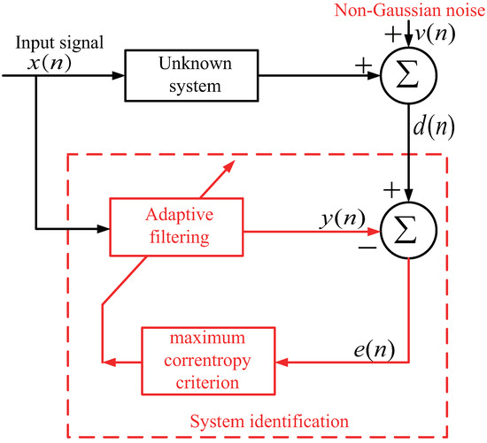
Figure 1.
A typical adaptive system identification scheme under the MCC method.
Herein, , represents norm, and we use .
To get the solution of Equation (3), the Lagrange multiplier (LM) method is used in this paper. Therefore, the MCC’s cost function is [27]:
where denotes Lagrange multiplier. Then, we have:
and
Thus, we can get the following formula:
Here, is obtained:
Compared to the basic LMS, an exponential weighting is considered and used in MCC, which is for eliminating the large errors. The MCC algorithm is robust for dealing with impulsive noises for system identifications.
2.2. Zero Attracting Technique
From the update equation in Equation (7), it is found that the MCC system identification method does not consider the sparse-structure information in the sparse system . Furthermore, the MCC-based system identification method can be written as [23,27]
In recent years, the zero attracting methods [10,27,28,29,30,31,32,33,34,35,36,37,38,39,40] have been widely studied to use the sparsity information in the FIR channels. These zero attracting algorithms are realized by integrating norm penalties, such as -norm and reweighted -norm [10], into the traditional AF algorithms. Thus, the zero attracting sparse MCC-based adaptive filters can be summarized as [10,27,28,29,30,31,32,33,34,35,36,37,38,39,40]
In Equation (9), the sparsity penalty term is usually given by introducing different norm penalties to utilize the prior sparse inform of these sparse systems [10,27,28,29,30,31,32,33,34,35,36,37,38,39,40]. Thus, the - and reweighted -norms are considered for exploiting the sparse MCCs to form ZA MCC (ZA-MCC) and reweighting ZA-MCC (RZA-MCC) algorithms [41]. Although the sparse MCCs achieve better estimation performance compared with the traditional MCC algorithm for identifying sparse systems, they are still needed to be improved for practical applications. Thus, we will develop a sparse NMCC algorithm by using the normalization method, proportionate-type method and the zero attracting techniques.
3. Proposed Proportionate NMCC Algorithms
3.1. Proportionate NMCC (PNMCC) Algorithm
In order to get the PNMCC, we reinvestigate the MCC in the AF framework again. Here, the NMCC is also rewritten in Equation (3). The differences between the MCC and NMCC algorithms are that we use in NMCC algorithm to replace the in the MCC. Similarly, the NMCC is to implement the following updating equation:
Then, we use a reweighting controlling matrix for reassigning different weights to the magnitudes of the filter coefficients, where the idea is obtained from the known Pt algorithms. Introducing into (10), we get
Here, represents a constant to get a stable solution. We know that a diagonal matrix is used to give a modification of NMCC’s step size under a rule given as follows. In general, is [2,3,4]
where the individual gain is
with
Here, and are constants, and they are usually set to be and [2]. is implemented to avoid the stalling. The parameter is used for preventing from stalling.
3.2. Proportionate NMCC with a CIM
Here, we first introduce the CIM theory [41,42,43,44,45,46,47,48,49,50]. As we know, the correntropy method is achieved from nonlinear measurement of random similar vectors and , which are in kernel space. Thus, we have
where represents the shift-invariant Mercer kernel, and represents the joint distribution of and , and is the expectation operation of . In general, the distribution of the data is usually unknown. Moreover, only a few samples of are available in practice. Thus, the correntropy can be obtained by [41,42,43,44,45,46,47,48,49,50]
According to the correntropy theory, the Gaussian kernel is a kind of typical kernel, which is given by [41,42,43,44,45,46,47,48,49,50]
where , and is the width of a kernel. The used correntropy has a boundary under various distributions and it can give robustness characteristics for non-Gaussian noise, which has been used for exploiting MCC algorithms.
Next, we give the CIM to better understand the correntropy theory. By considering and in a sampling space, we can define the CIM as [41,42,43,44,45,46,47,48,49,50]
where . Thus, we can get
It can be seen that, if , then, as , we found that the CIM is an -norm approximation, and is set to be a very small constant.
Finally, we propose a CIM penalized PNMCC (CIM-PNMCC) algorithm, which is realized by introducing CIM penalty into PNMCC’s cost function to construct a sparse PNMSS with a implementation of the CIM. We also take the gain controlling matrix into consideration to design the desired zero-attractor. According to the zero attracting sparse AF algorithms, the developed CIM-PNMCC is to calculate
where denotes the inverse operation of . is a regularization, which is a balance between the system identification errors and CIM penalty of . Our devised CIM-PNMCC is different from the general zero attracting since it provides a scaling by on the CIM penalty.
To get the minimization of (20), the LM method is employed. Therefore, the proposed CIM-PNMCC’s cost function is
Multiplying on both sides of Equation (23), we get
Considering Equation (22), we obtain
The Lagrange multiplier is obtained
From the updated Equation (27), we can see that the elements in are very small in comparison with 1. Thus, we can ignore this term, and the proposed CIM-PNMCC’s updating equation is
We introduce a step-size and . Then, the proposed CIM-PNMCC’s updating equation is changed to be
where , and is a regularization parameter used for controlling the zero attracting strength. Similar to the early reported zero attracting algorithms, there is an additional term in the CIM-PNMCC algorithm, which is called a CIM zero-attractor. In the devised CIM-PNMCC, the constructed CIM zero-attractor attracts small coefficients to zero with a high probability. Furthermore, our proposed CIM-PNMCC algorithm employs a gain controlling matrix to assign a large step-size for the dominant coefficients, while the zero attractor mainly gives a strong zero-attraction to the inactive coefficients. Therefore, our CIM-PNMCC algorithm has the advantages of the proportionate-type algorithms, normalized adaptive filtering algorithms and zero attraction adaptive filters.
From the derivation of the CIM-PNMCC, we can put the remarks as follows:
- A PNMCC algorithm is devised by using a generalized Gaussian distribution function to utilize the prior-sparse-structure information in the in-nature systems.
- A CIM constraint is adopted and incorporated into the proposed PNMCC’s cost function to create a modified cost function.
- The derivation of the devised CIM-PNMCC algorithm is presented by the use of the LM method to further take the advantages of the prior-sparse-structure information.
- The convergence of the CIM-PNMCC is analyzed and its performance is discussed for identifying sparse systems, which is compared with the previous MCC algorithms.
- Our developed CIM-PNMCC outperforms the previous MCC algorithms in terms of the convergence and MSD.
4. Convergence Analysis of the Devised CIM-PNMCC
The mean and convergence for the CIM-PNMCC is performed based on an approximation approach. For simple description, our proposed CIM-PNMCC is rewritten as
where and . For simple convergence analysis, we give some assumptions that are used frequently in [51,52,53,54].
We have the following assumptions (A): A1: with zero mean is i. i. d.
A2: is independent with , and it is zero mean, and its variance is .
A3: is independent with .
A4: and are independent with .
A5: The expectation of a ration of two random variables is equal to the ration of the expectation of each random variable. Moreover, the expectation is existing, and , and [55].
4.1. Mean Convergence
A misalignment vector is defined by
Taking the expectation on Equation (32) and using the A1, A2, A3 and A5, we get
where represents the auto-correlation matrix. Based on the symmetric and positive semidefinite property of the , we have
where is the eigenvalue matrix. Next, premultiplying on both sides of Equation (33), and considering unitarians, we get
where , and represents a diagonal. is bounded [41] and every element of is independent. Hence, converges to zero if and only if . As a result, our CIM-PNMCC algorithm converges only if it converges for the . Since , where is matrix trace operation, converges to zero when meets
Using A1 and A3, we have . Moreover, considering , and , we obtain
4.2. Mean Square Convergence (MSC)
As for the MSC of our CIM-PNMCC, we give the auto-covariance of
where
Under the assumptions 1–5, we can say that and are both zero means. In addition, we know that , and are independent with each other. Putting Equation (40) into Equation (38), we have
where . Since the Gaussian variable with fourth-order moment is three times the variable square [52], and we also know that is symmetric [52], we obtain
In Equation (45), , , and are all bounded. Thus, is converged. Then, the CIM-PNMCC is stable when
By solving the Equation (46), we can get the range of
5. Results and Discussions of the PNMCC and CIM-PNMCC Algorithms
We will discuss the behavior of our proposed PNMCC and CIM-PNMCC for identifying sparse systems. Furthermore, their system identification performance is analyzed by comparing with NMCC, MCC, RZA-MCC and ZA-MCC algorithms. Additionally, the PNLMS algorithm is also employed for estimation performance comparison since the MCC is an LMS-like algorithm and the PNLMS is a proportionate-typed NLMS, which is also a PNMCC-like algorithm. The MSD is employed for evaluating the behaviors of the devised PNMCC and CIM-PNMCC algorithms, defining by
Based on the derivation of the PNMCC and CIM-PNMCC algorithms, gives an important effect on the PNMCC algorithm, while and play important effects on the CIM-PNMCC algorithm. Thereby, we first investigate their effects on the estimation behaviors over sparse systems with impulsive noise. In this paper, is used for generating the desired noise, where are the Gaussian distributions with means of and variances of , where is a mixture parameter. Herein, a sparse system with a length of is adopted. One non-zero tap randomly distributes in the system. To investigate the effects of on the PNMCC algorithm, the simulation parameters are and with corresponding results presented in Figure 2. The developed PNMCC converges faster when increases from to , which has a similar function in the PNLMS algorithm to implement the step-size.
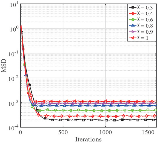
Figure 2.
Effects on the PNMCC algorithm with different .
Similarly, the parameter is also selected to understand the performance of the derived CIM-PNMCC, whose performance is described in Figure 3. The CIM-PNMCC’s convergence speed rate becomes faster when increases from 0.2 to 0.7. However, the estimation misalignment is getting worse with an increment of . Additionally, is a zero attraction controlling parameter, which is designed to trade off the sparsity development and estimation bias. The effects of on the CIM-PNMCC estimation behavior is illustrated in Figure 4. It is observed that the estimation bias of the CIM-PNMCC is reduced as ranges from to . If is reduced from to , the estimation bias rebounds towards the opposite direction. Therefore, we should choose proper parameter value to obtain good performance of the PNMCC and CIM-PNMCC algorithms.
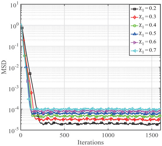
Figure 3.
Effects on the CIM-PNMCC algorithm with different .
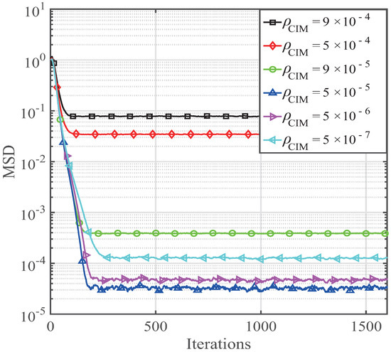
Figure 4.
Behaviors the CIM-PNMCC algorithm with different .
Then, these parameters are used to obtain the convergence speed investigation of the developed PNMCC and CIM-PNMCC algorithms. Here, , , , , , , , , , , where , , , , are step-sizes for NMCC, MCC, RZA-MCC, ZA-MCC and PNLMS algorithms. and are the regularization parameters for RZA-MCC and ZA-MCC, respectively. The convergence comparisons for PNMCC and CIM-PNMCC algorithms are given in Figure 5. From Figure 5, we observe that the PNMCC converges faster than the PNLMS and NMCC algorithms. It is worth noting that our developed CIM-PNMCC gets the fastest convergence speed for adaptive system identifications. The CIM-PNMCC algorithm only needs 200 iterations to reach a steady-state MSD, while the previously reported RZA-MCC algorithm requires more than 400 iterations to get its steady-state MSD. Thereby, the CIM-PNMCC algorithm converges much quicker than the RZA-MCC algorithm for achieving the same MSD.
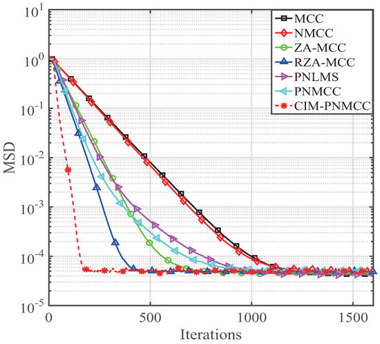
Figure 5.
Convergence of the PNMCC and CIM-PNMCC algorithms.
Next, the effects of the sparsity level are analyzed by using the non-zero coefficients K in the FIR system. Here, we still use a 16 length sparse system that has K dominant coefficients. The simulated parameters for the mentioned adaptive filtering algorithms are , , , , , , , , . The estimation behavior of our developed PNMCC and CIM-PNMCC algorithms is discussed for various K, and their estimation behaviors are given in Figure 6, Figure 7, Figure 8 and Figure 9, respectively. It is noted that our developed PNMCC achieves a little gain compared with the PNLMS because they have comparable complexity and similar updating equation except the exponential weighting. However, our PNMCC algorithm achieves lower steady-state bias for . As for the CIM-PNMCC, it provides the lowest steady-state misalignment because it has a zero attraction term that can quickly force inactive coefficients to zero. With an increase of K, the MSD floor is increased. However, our developed CIM-PNMCC still provides the lowest steady-state misalignment, indicating that the CIM-PNMCC is more useful. Even for , our CIM-PNMCC algorithm can still get an MSD level of , which is a very low estimation bias. As we know, the ZA-MCC is a regular zero attraction algorithm. However, with the increasing of K, we can see that the performance of the ZA-MCC has degraded because of its uniform zero attraction on all the channel coefficients.
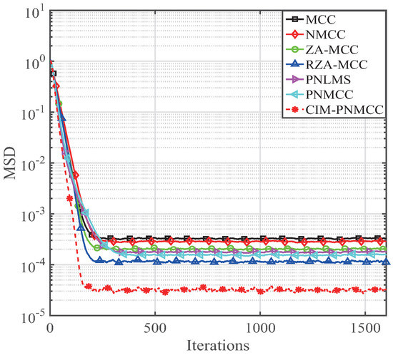
Figure 6.
Behaviors of the PNMCC and CIM-PNMCC algorithms for .
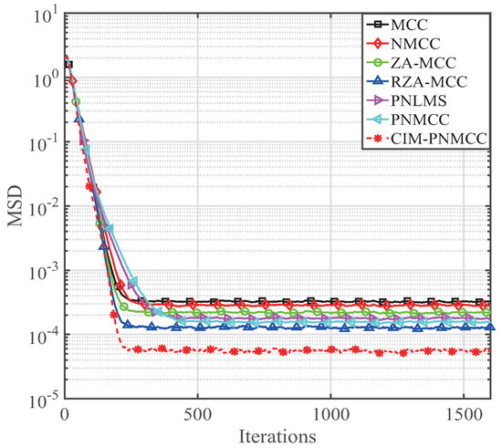
Figure 7.
Behaviors of the PNMCC and CIM-PNMCC algorithms for .
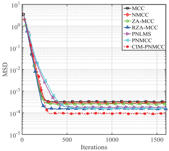
Figure 8.
Behaviors of the PNMCC and CIM-PNMCC algorithms for .
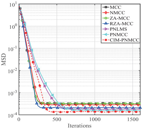
Figure 9.
Behaviors of the PNMCC and CIM-PNMCC algorithms for .
Then, we construct an example to discuss the tracking behavior of our devised PNMCC and CIM-PNMCC algorithms. Herein, we investigate their tracking performance over network echo channels with different sparsities, and the channel length is set to be 256. We use to measure the sparsity of the designated network echo channel [37]. A typical network echo channel is given in Figure 10. The simulation parameters used in this experiment are , , , , , , , , . The tracking behavior for and is illustrated in Figure 10. Our PNMCC algorithm outperforms the PNLMS, MCC and NMCC algorithms in terms of the estimation bias for . However, our PNMCC algorithm achieves the similar tracking behavior to the PNLMS algorithm because of the weighted step-size assignment scheme. For our developed CIM-PNMCC, it possesses the fastest convergence speed and lowest MSD for both and . Therefore, a conclusion is given that our developed PNMCC and CIM-PNMCC algorithms can be used to effectively handle the sparse system identification. Furthermore, the CIM-PNMCC algorithm has little effect on the sparsity of compared with the mentioned algorithms above.
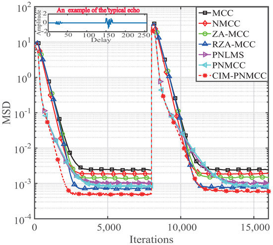
Figure 10.
Tracking behaviors of the PNMCC and CIM-PNMCC algorithms for estimating an echo channel (An example of typical echo channel is also included on the top of this figure.).
Finally, a practical speech is considered as the input signal to test the performance of the devised CIM-PNMCC. In this experiment, the used speech signal is a 2 s real speech, which has a sampling ratio of 8 kHz. The parameter used herein is the same as the last experiment. The speech signal, as well as the results, are shown in Figure 11 and Figure 12, respectively. The proposed CIM-PNMCC can still get the best convergence speed and lower estimation error for echo cancellation applications.
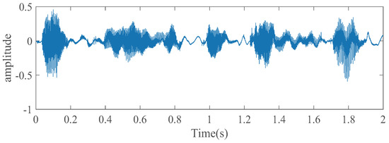
Figure 11.
Speech signal used in the experiment.
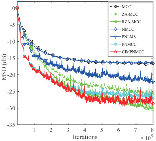
Figure 12.
Performance of the CIM-PNMCC for sparse echo response with speech input.
According to the aforementioned discussion of the proposed PNMCC and CIM-PNMCC algorithms, the CIM-PNMCC achieves the smallest estimation misalignment and quickest convergence compared with the mentioned adaptive system identification algorithms. For the proposed PNMCC algorithm, it has a similar complexity to the PNLMS, while it can provide a little better gain than the PNLMS in impulsive noise environments. Moreover, the CIM-PNMCC performs better than the PNMCC since it introduces a CIM zero-attractor to use the sparsity characteristics in the used systems. This is attributed to the CIM measurement which can account for the dominant non-zero coefficients. In addition, the CIM zero attractor forces the inactive coefficients to zero rapidly. Additionally, the developed CIM-PNMCC algorithm has an additional regularization parameter that is used for controlling the zero attraction ability.
6. Conclusions
PNMCC and CIM-PNMCC algorithms were developed, and their behaviors were presented and discussed for sparse system identification. The CIM-PNMCC algorithm can provide the fastest convergence, while the PNMCC also performs better than the PNLMS algorithm. Since the CIM-PNMCC algorithm integrates a CIM zero attraction in its iteration, its convergence is faster and its estimation bias is smaller than the presented PNMCC algorithm. The obtained results showed that the CIM-PNMCC is stable, and it can obtain more gains. Therefore, the proposed CIM-PNMCC is a good candidate to consider the practical applications for sparse system identifications. For the future work, we will develop the block sparse PNMCC algorithm based on the block method in [56,57] and reduce the complexity of the proposed CIM-PNMCC algorithm.
Author Contributions
Y.L. proposed the idea and coded for the algorithms, and wrote a draft. Y.W. did the analysis of the simulation and the convergence analysis. L.S. checked the code and simulations. All of the authors cooperatively finished this paper together.
Funding
This work was partially supported by the National Key Research and Development Program of China (2016YFE0111100), Key Research and Development Program of Heilongjiang (GX17A016), the Science and Technology innovative Talents Foundation of Harbin (2016RAXXJ044), the Natural Science Foundation of Beijing (4182077) and China Postdoctoral Science Foundation (2017M620918), and the PhD Student Research and Innovation Fund of the Fundamental Research Funds for the Central Universities (HEUGIP201707), and the Opening Fund of Acoustics Science and Technology Laboratory (Grant No. SSKF2016001).
Conflicts of Interest
The authors declare no conflict of interest.
References
- Naylor, P.A.; Cui, J.; Brookes, M. Adaptive algorithms for sparse echo cancellation. Signal Process. 2009, 86, 1182–1192. [Google Scholar] [CrossRef]
- Duttweiler, D.L. Proportionate normalized least-mean-squares adaptation in echo cancelers. IEEE Trans. Speech Audio Peocess. 2000, 8, 508–518. [Google Scholar] [CrossRef]
- Li, Y.; Hamamura, M. An improved proportionate normalized least-mean-square algorithm for broadband multipath channel estimation. Sci. World J. 2014, 2014, 572969. [Google Scholar] [CrossRef] [PubMed]
- Benesty, J.; Gay, S.L. An improved PNLMS algorithm. In Proceedings of the 2002 IEEE International Conference on Acoustics, Speech, and Signal Processing, ICASSP’02, Orlando, FL, USA, 13–17 May 2002; Volume II, pp. 1881–1884. [Google Scholar]
- Hunt, K.J.; Sbarbaro, D. Adaptive filtering and neural networks for realisation of internal model control. Intell. Syst. Eng. 1993, 2, 67–76. [Google Scholar] [CrossRef]
- Kumar, A.M.P.; Ramesha, K. Adaptive filter algorithms based noise cancellation using neural network in mobile applications. In Proceedings of the International Conference on Intelligent Computing and Applications, Canberra, Australia, 20–23 January 2017; pp. 67–68. [Google Scholar]
- Kakareka, J.W.; Faranesh, A.Z.; Pursley, R.H.; Campbell-Washburn, A.; Herzka, D.A.; Rogers, T.; Kanter, J.; Ratnayaka, K.; Lederman, R.J.; Pohida, T.J. Physiological recording in the MRI environment (PRiME): MRI-compatible hemodynamic recording system. IEEE J. Transl. Eng. Health Med. 2018, 2018, 4100112. [Google Scholar] [CrossRef] [PubMed]
- Gui, G.; Adachi, F. Improved least mean square algorithm with application to adaptive sparse channel estimation. EURASIP J. Wirel. Commun. Netw. 2013, 2013, 204. [Google Scholar] [CrossRef]
- Li, Y.; Zhang, C.; Wang, S. Low complexity non-uniform penalized affine projection algorithm for sparse system identification. Circuit Syst. Signal Process. 2016, 35, 1611–1624. [Google Scholar] [CrossRef]
- Chen, Y.; Gu, Y.; Hero, A.O. Sparse LMS for system identification. In Proceedings of the 2009 IEEE International Conference on Acoustics, Speech and Signal Processing, ICASSP’09, Taipei, Taiwan, 19–24 April 2009; pp. 3125–3128. [Google Scholar]
- Cotter, S.F.; Rao, B.D. Sparse channel estimation via matching pursuit with application to equalization. IEEE Trans. Commun. 2002, 50, 374–377. [Google Scholar] [CrossRef]
- Deng, H.; Doroslovacki, M. Improving convergence of the PNLMS algorithm for sparse impulse response identification. IEEE Signal Process. Lett. 2005, 12, 181–184. [Google Scholar] [CrossRef]
- Das, R.L.; Chakraborty, M. A zero attracting proportionate normalized least mean square algorithm. In Proceedings of the 2012 Asia Pacific Signal and Information Processing Association Annual Summit and Conference, APSIPA ASC’12, Hollywood, CA, USA, 3–6 December 2012; pp. 1–4. [Google Scholar]
- Deng, H.; Doroslovacki, M. Proportionate adaptive algorithms for network echo cancellation. IEEE Trans. Signal Process. 2006, 54, 1794–1803. [Google Scholar] [CrossRef]
- Paleolohu, C.; Ciochina, S.; Benesty, J. An efficient proportionate affine projection algorithm for echo cancellation. IEEE Signal Process. Lett. 2010, 17, 165–168. [Google Scholar] [CrossRef]
- Wu, Z.; Peng, S.; Chen, B.; Zhao, H.; Principe, J.C. Proportionate minimum error entropy algorithm for sparse system identification. Entropy 2015, 17, 5995–6006. [Google Scholar] [CrossRef]
- Chen, B.; Zhu, Y.; Hu, J.; Principe, J.C. System Parameter Identification: Information Criteria and Algorithms; Elsevier: Amsterdam, The Netherlands, 2013. [Google Scholar]
- Wolsztynski, E.; Thierry, E.; Pronzato, L. Minimum-entropy estimation in semi-parametric models. Signal Process. 2005, 85, 937–949. [Google Scholar] [CrossRef]
- Chen, B.; Principe, J.C. Some further results on the minimum error entropy estimation. Entropy 2012, 14, 966–977. [Google Scholar] [CrossRef]
- Chen, B.; Principe, J.C. On the smoothed minimum error entropy Criterion. Entropy 2012, 14, 2311–2323. [Google Scholar] [CrossRef]
- Xue, Y.; Zhu, X. The minimum error entropy based robust wireless channel tracking in impulsive noise. IEEE Commun. Lett. 2002, 6, 228–230. [Google Scholar]
- Liu, W.F.; Pokharel, P.P.; Principe, J.C. Correntropy: Properties and applications in nonGaussian signal processing. IEEE Trans. Signal Process. 2007, 55, 5286–5298. [Google Scholar] [CrossRef]
- Singh, A.; Principe, J.C. Using correntropy as a cost function in linear adaptive filters. In Proceedings of the 2009 International Joint Conference on Neural Networks, IJCNN’09, Atlanta, GA, USA, 14–19 June 2009; pp. 2950–2955. [Google Scholar]
- Palmieri, F.A.N.; Ciuonzo, D. Objective priors from maximum entropy in data classification. Inf. Fusion 2013, 14, 186–198. [Google Scholar] [CrossRef]
- Debbah, M.; Muller, R.R. MIMO channel modeling and the principle of maximum entropy. IEEE Trans. Inf. Theory 2005, 51, 1667–1690. [Google Scholar] [CrossRef]
- Palmieri, F.; Ciuonzo, D. Data fusion with entropic priors. In Proceedings of the 20th Italian Workshop on Neural Nets, Vietri sul Mare, Salerno, Italy, 27–29 May 2011; Volume 226, pp. 107–114. [Google Scholar]
- Li, Y.; Wang, Y.; Yang, R.; Albu, F. A soft parameter function penalized normalized maximum correntropy criterion algorithm for sparse system identification. Entropy 2017, 19, 45. [Google Scholar] [CrossRef]
- Gu, Y.; Jin, J.; Mei, S. L0 norm constraint LMS algorithms for sparse system identification. IEEE Signal Process. Lett. 2009, 16, 774–777. [Google Scholar]
- Taheri, O.; Vorobyov, S.A. Sparse channel estimation with Lp-norm and reweighted L1-norm penalized least mean squares. In Proceedings of the IEEE International Conference on Acoustics, Speech, and Signal Processing, ICASSP 2011, Prague, Czech Republic, 22–27 May 2011; pp. 2864–2867. [Google Scholar]
- Li, Y.; Wang, Y.; Jiang, T. Sparse channel estimation based on a p-norm-like constrained least mean fourth algorithm. In Proceedings of the 2015 International Conference on Wireless Communications & Signal Processing (WCSP) WCSP’15, Nanjing, China, 15–17 October 2015. [Google Scholar]
- Li, Y.; Hamamura, M. Zero-attracting variable-step-size least mean square algorithms for adaptive sparse channel estimation. Int. J. Adapt. Control Signal Process. 2015, 29, 1189–1206. [Google Scholar] [CrossRef]
- Li, Y.; Li, W.; Yu, W.; Wan, J.; Li, Z. Sparse adaptive channel estimation based on lp-norm-penalized affine projection algorithm. Int. J. Antennas Propag. 2014, 2014, 434659. [Google Scholar] [CrossRef]
- Li, Y.; Jin, Z.; Wang, Y.; Yang, R. A robust sparse adaptive filtering algorithm with a correntropy induced metric constraint for broadband multi-path channel estimation. Entropy 2016, 18, 380. [Google Scholar] [CrossRef]
- Gui, G.; Peng, W.; Adachi, F. Sparse least mean fourth algorithm for adaptive channel estimation in low signal-to-noise ratio region. Int. J. Commun. Syst. 2014, 27, 3147–3157. [Google Scholar] [CrossRef]
- Li, Y.; Wang, Y.; Jiang, T. Norm-adaption penalized least mean square/fourth algorithm for sparse channel estimation. Signal Process. 2016, 128, 243–251. [Google Scholar] [CrossRef]
- Gui, G.; Xu, L.; Matsushita, S. Improved adaptive sparse channel estimation using mixed square/fourth error criterion. J. Frankl. Inst. 2015, 352, 4579–4594. [Google Scholar] [CrossRef]
- Li, Y.; Wang, Y.; Jiang, T. Sparse-aware set-membership NLMS algorithms and their application for sparse channel estimation and echo cancelation. AEU-Int. J. Electron. Commun. 2016, 70, 895–902. [Google Scholar] [CrossRef]
- Gui, G.; Mehbodniya, A.; Adachi, F. Least mean square/fourth algorithm for adaptive sparse channel estimation. In Proceedings of the 2013 IEEE 24th Annual International Symposium on Personal, Indoor, and Mobile Radio Communications (PIMRC), London, UK, 8–11 September 2013; pp. 296–300. [Google Scholar]
- Albu, F.; Gully, A.; de Lamare, R.C. Sparsity-aware pseudo affine projection algorithm for active noise control. In Proceedings of the 2014 Asia-Pacific Signal and Information Processing Association Annual Summit and Conference (APSIPA), Siem Reap, Cambodia, 9–12 December 2014; pp. 1–5. [Google Scholar]
- Li, Y.; Wang, Y.; Jiang, T. Sparse least mean mixed-norm adaptive filtering algorithms for sparse channel estimation application. Int. J. Commun. Syst. 2016, 30. [Google Scholar] [CrossRef]
- Ma, W.; Qu, H.; Gui, G.; Xu, L.; Zhao, J.; Chen, B. Maximum correntropy criterion based sparse adaptive filtering algorithms for robust channel estimation under non-Gaussian environments. J. Frankl. Inst. 2015, 352, 2708–2727. [Google Scholar] [CrossRef]
- Chen, B.; Principe, J.C. Maximum correntropy estimation is a smoothed MAP estimation. IEEE Signal Process. Lett. 2012, 19, 491–494. [Google Scholar] [CrossRef]
- Chen, B.; Xing, L.; Liang, J.; Zheng, N.; Principe, J.C. Steady-state mean-square error analysis for adaptive filtering under the maximum correntropy criterion. IEEE Signal Process. Lett. 2014, 21, 880–884. [Google Scholar]
- Wu, Z.; Peng, S.; Chen, B.; Zhao, H. Robust Hammerstein adaptive filtering under maximum correntropy criterion. Entropy 2015, 17, 7149–7166. [Google Scholar] [CrossRef]
- Huijse, P.; Estevez, P.A.; Zegers, P.; Principe, J.C.; Protopapas, P. Period estimation in astronomical time series using slotted correntropy. IEEE Signal Process. Lett. 2011, 18, 371–374. [Google Scholar] [CrossRef]
- Li, Y.; Wang, Y. Sparse SM-NLMS algorithm based on correntropy criterion. IET Electron. Lett. 2016, 52, 1461–1463. [Google Scholar] [CrossRef]
- Zhao, S.; Chen, B.; Principe, J.C. Kernel adaptive filtering with maximum correntropy criterion. In Proceedings of the 2011 International Joint Conference on Neural Networks IJCNN, San Jose, CA, USA, 31 July–5 August 2011; pp. 2012–2017. [Google Scholar]
- Chen, B.; Xing, L.; Zhao, H.; Zheng, N.; Principe, J.C. Generalized correntropy for robust adaptive filtering. IEEE Trans. Signal Process. 2016, 64, 3376–3387. [Google Scholar] [CrossRef]
- Chen, B.; Wang, J.; Zhao, H.; Zheng, N.; Principe, J.C. Convergence of a fixed-point algorithm under maximum correntropy criterion. IEEE Signal Process. Lett. 2015, 22, 1723–1727. [Google Scholar] [CrossRef]
- Seth, S.; Principe, J.C. Compressed signal reconstruction using the correntropy induced metric. In Proceedings of the 2008 IEEE International Conference on Acoustics, Speech and Signal Processing ICASSP’08, Las Vegas, NV, USA, 31 March–4 April 2008; pp. 3845–3848. [Google Scholar]
- Aliyu, M.L.; Alkassim, M.A.; Salman, M.S. A lp-norm variable step-size LMS algorithm for sparse system identification. Signal Image Video Process. 2015, 9, 1559–1565. [Google Scholar] [CrossRef]
- Shi, K.; Shi, P. Convergence analysis of sparse LMS algorithms with l1-norm penalty based on white input signal. Signal Process. 2010, 90, 3289–3293. [Google Scholar] [CrossRef]
- Salman, M.S. Sparse leaky-LMS algorithm for system identification and its convergence analysis. Int. J. Adapt. Control Signal Process. 2015, 28, 1065–1072. [Google Scholar] [CrossRef]
- Ma, W.; Zheng, D.; Zhang, Z. Robust proportionate adaptive filter based on maximum correntropy criterion for sparse system identification in impulsive noise environments. Signal Image Video Process. 2018, 12, 117–124. [Google Scholar] [CrossRef]
- Petraglia, M.R.; Haddad, D.B. Transient and steady-state MSE analysis of the IMPNLMS algorithm. Digit. Signal Process. 2014, 33, 50–59. [Google Scholar]
- Li, Y.; Jiang, Z.; Osman, O.; Han, X.; Yin, J. Mixed norm constrained sparse APA algorithm for satellite and network channel estimation. IEEE Access 2018, 6, 65901–65908. [Google Scholar] [CrossRef]
- Li, Y.; Jiang, Z.; Jin, Z.; Han, X.; Yin, J. Cluster-sparse proportionate NLMS algorithm with the hybrid norm constraint. IEEE Access 2018, 6, 47794–47803. [Google Scholar] [CrossRef]
© 2018 by the authors. Licensee MDPI, Basel, Switzerland. This article is an open access article distributed under the terms and conditions of the Creative Commons Attribution (CC BY) license (http://creativecommons.org/licenses/by/4.0/).