1. Introduction
Symmetric graphs have many real-life applications as vehicle routing, warehouse logistics, planning circuit boards, virtual networking [
1,
2,
3,
4]. The goal of the base Symmetric Traveling Salesman Problem (sTSP) is to find the shortest Hamiltonian cycle in a graph. The Hamiltonian cycle visits each vertex exactly once. The length of the path is calculated with the sum of the corresponding edge weights. The weight values of the graph edges, in general case, are given with a squared matrix of non-negative values. In this paper, we are focusing on Euclidean TSP (eTSP) problems where the graph nodes correspond to points in the Euclidean metric space and the weights are equal to the Euclidean distances between these points. In this case we get a symmetric distance matrix. The generation of the shortest Hamiltonian cycle is an NP-hard problem [
5] usually formulated as an integer linear programming problem [
6].
Regarding the complexity of the sTSP, two different problems are usually investigated: the Decision problem (DTSP) and the Optimization problem (OTSP). DTSP aims to determine whether a Hamiltonian cycle of length not greater than a given value exists. The goal of OTSP is to find the Hamiltonian cycle of minimal length.
In the brute-force solution method, all possible permutations of the nodes are tested to select the optimal route. This approach requires
O(
N!) execution cost. Regarding the other alternative exact solution methods, we can emphasize the integer linear programming approach and the Held-Karp algorithm. In the case of integer linear programming formulation [
7], we have
O(
N2) variables and subtour elimination constraints. As a direct solution is unfeasible, the model is relaxed to find a solution. In the proposal [
8] a novel representation form was introduced to reduce the number of subtour elimination constraints. In Reference [
9], the related integer linear programming problem is based on the two-commodity network flow formulation of the TSP.
The Held-Karp method [
10] uses the dynamic programming approach. The algorithm follows the idea of successive approximation; the global problem is decomposed into a set of related subproblems and the optimal solutions of the subproblems are composed into an optimal global solution. Although, this method provides a better time cost efficiency than the brute-force algorithm, it belongs to exponential complexity class, having a worst-case cost
O(2
NN2). Another drawback of the method is that it raises a significant space requirement too.
In Reference [
11] the branch-and-bound approach was implemented to determine the exact optimal tour. The method builds up a state-tree that manages the paths already processed. Each node stores a path description together with its cost values involving a lower bound cost value too. The construction of the state tree requires
O(
N!) costs in the worst case. In the [
12] a genetic node is assigned to an assignment problem. The related subtours are broken by creating subproblems in which all edges of the subtour are prohibited.
Due to high computational costs of the exact solution methods, the heuristic optimization of sTSP is one of the most widely investigated combinatorial optimization problem. One group of the heuristic methods use algorithms for direct route construction. As the main goal is to minimize the sum of a fixed number of edge weights, a sound heuristic is to minimize the components in the sum. Thus, the constructional heuristic methods are in general aimed for selecting the edges of minimal length. In the case of Nearest Neighbour method [
13], the algorithm starts with a random selection of a vertex. In each iteration step, the nearest free vertex is selected and it will be connected to the current node. In the Greedy Edge Insertion heuristic method [
14], the edges are ordered by their weight values. The algorithm inserts the shortest available edge into the route in every iteration step. During the construction process there are two constraints to be met: (a) any node is connected to exactly two other nodes; (b) no cycle can exist with less than N edges. The Greedy Vertex Insertion algorithm [
15] extends the existing route with a vertex having the lowest cost increase. A similar approach was implemented in the Boruvka algorithm [
16] where the edges are processed in length order. An edge with minimal length is inserted into the tour if it does not affect the integrity of the current route.
The Fast Recursive Partitioning method [
17] performs a hierarchical clustering of the nodes corresponding to points in the Euclidean space. The points are structured into a hierarchical tree, similarly to the R-tree structure. The leaf nodes contain a smaller number of points, with a given capacity. In first phase, the algorithm performs a TSP route generation for each of the leaf buckets and in the second phase, the local routes are merged into a global tour. The Karp’s Partitioning Heuristic [
18] is based on a similar hierarchical decomposition technique but it uses a more sophisticated patch-based method. The Double Minimum Spanning Tree algorithm [
19] and its improved version, the Christofides Algorithm [
20], generates first a minimal spanning tree for the input graph and adjusts this tree with a minimum-weight matching.
Another family of heuristic methods aims at the improvement of existing solutions found so far. Having one or more initial suggestions, the algorithm tries to find a better solution. The improvement heuristics can achieve significantly better results than the direct construction methods [
6]. These algorithms use iterations and random search components; thus the execution time is here usually higher. The k-opt method [
21] belongs to the family of local search heuristics. Similarly to the string edit distance, a tour distance is defined between two edge sequences. The tour t’ is considered in the k-neighbourhood of t if the distance between t and t’ is not greater than
k. Having an initial tour, this method repeatedly replaces the current tour with a tour in its neighbourhood providing a smaller tour length. Due to the higher time cost of the neighbourhood construction process, the variants with lower k values (2-opt and 3-opt) are preferred in the practical implementations.
The Lin-Kernighan [
22] algorithm improves the efficiency of the standard k-opt approaches by using a flexible neighbourhood construction. The method first determines the optimal
k value for the k-opt method and performs the search operation in the dynamic k-neighbourhood environment, where each move is composed of special 2-opt and 3-opt moves. As the quality of the base Lin-Kernighan local optimization methods depends significantly on the quality of the initial route, a usual approach is to repeat the local search with different initial routes and return the best result. The approach presented by [
23] uses a different idea to work harder on the current tours using kicks on the tour found by Lin-Kernighan. The resulting algorithm is known as Chained Lin-Kernighan method.
There are also approaches using generic Evolutionary Optimization [
24] methods for the shortest tour problem. Such a method generates a set of initial tours and using the route length as a fitness function, the next generation is produced with the application of the reproduction, crossover and mutation operators. As the mutation and crossover has a random nature, the quality of the result is weak for large search space problems. In Reference [
25], the predictability of TSP optimization is investigated analysing different bacterial evolutionary algorithms with local search.
In the Multi-level Approach [
26], the tour is constructed with a hierarchy of increasingly coarse approximations. Having an initial problem on
N nodes, the algorithm first fixes an edge at every level, thus the next level optimizes a problem of smaller size having only (
N − 1) nodes. After generating an initial tour, a usual refinement phase is executed to improve the tour quality. The Tour-merging Method [
27] is based on the observation that the routes of good quality usually share a large set of common edges. The algorithm uses specific heuristics to generate near-optimal tours and dynamic programming to unify the partial solutions into a common solution.
There is a rich literature on detailed analysis and performance comparison of the main heuristic methods (Nearest Neighbour, Nearest Insertion, Tabu Search, Lin-Kernighan, Greedy, Boruvka, Savings and Genetic Algorithm). Based on the results presented in Reference [
16,
19,
28]: (a) the fastest algorithms are the Greedy and Savings method but they provide an average tour quality; (b) the Nearest Neighbour and Nearest Insertion algorithms are dominated by the Greedy and Savings methods both in time and tour quality factors; (c) the best route quality can be achieved by the application of 3-opt/5-opt methods (Lin-Kernighan and Helsgaun); (d) considering both the time and tour quality, the Chained Lin-Kernighan algorithm proves the best performance; (e) the Evolutionary and Swarm optimization methods are dominated by the k-opt methods both in time and tour quality factors; (f) the Tour-merging methods applied on the Chained Lin-Kernighan algorithm can improve the tour quality at some level but it requires a significantly higher time cost.
Most of the available heuristic methods work in a batch mode, where the full graph is presented as input. In this case the algorithm can get all information already at the start of the tour generation. An alternative approach is the incremental mode where the graph is initially empty and it is extended with new nodes incrementally. This can happen in some application areas as knowledge engineering or transportation problems where new concepts/locations can be added to the existing network. Having only a batch algorithm, after the insertion of a new node, we should rerun the full optimization process to get the new optimal tour. In these cases the incremental algorithms can provide a better solution than the standard batch methods.
Considering the main heuristic methods, only few can be adapted to the incremental construction approach. In the family of constructional heuristic methods, the methods usually process the edges in some selected order. For example, in Greedy Edge Insertion heuristic method [
14] or in Boruvka algorithm [
16], the edges are sorted by the length value. Greedy Vertex Insertion algorithm [
15] extends the existing route with a vertex having the lowest cost increase. In the case of Nearest Neighbour method [
13], the shortest free edge is selected related to the actual node. In all cases, if we extend the graph with a random new element and process this element with the mentioned methods, the resulted route will be usually suboptimal. In a batch mode, this element would be processed in an earlier step. The heuristics methods form the other groups use such operations (improvements, hierarchical decomposition) which are defined on the complete graph or on a complete subgraph.
In this paper, we propose a novel algorithm, called IntraClusTSP that can be used in Euclidean TSP for both incremental tour construction and tour refinement. The method first selects one or more clusters in the object graph and then it performs cluster-level route optimization for each cluster. In the final step, the optimized local routes are merged with the current global route yielding a new optimal route. This approach is based on the observation that adjacent nodes in the shortest Hamiltonian cycle in eTSP are usually nearest neighbour nodes. The IntraClusTSP refinement method provides a general framework for route optimization as it can use any current TSP methods to perform cluster level optimization. In our model, we use Chained Lin-Kernighan method for local optimization. The clusters selected for refinement may be overlapping clusters. Based on the performed tests, the proposed method provides superior efficiency for incremental route construction.
The rest of this paper is structured as follows. In the next section, a survey on TSP heuristics using incremental or cluster-based optimization is presented.
Section 3 presents the motivation for the development of the proposed IntraClusTSP method, the formal model and the constructed algorithms.
Section 4 focuses on its cost model and cost analysis. It presents the test results of the empirical efficiency comparison of the proposed method with the several TSP solution algorithms.
Section 5 demonstrates the application of IntraClusTSP algorithm in solving of a data analysis problem.
2. Incremental and Segmentation-Based Approaches in Solving eTSP
In the TSP terminology, the term incremental insertion heuristic refers to methods where the optimal tour is constructed by extension steps where in each step, the route is extended with a single node. The most widely known methods of this group are Nearest point insertion [
29], Furthest point insertion [
30] or Random point insertion [
31]. Based on the literature, the Furthest point insertion provides the best tour length. In this case, the point
x as the solution of
is selected to be inserted. In the formula,
T denotes the current route and
T″ is its complement. In our problem domain, this method is not suitable, as in every insertion cycle, the
T″ set contains only one node, the rest nodes are not known yet. Similarly, the Nearest point insertion method selects the nearest node from the points not linked into the tour yet. Thus, only the Random insertion heuristic can be used for our problem domain.
Considering the approximation efficiency of the insertion algorithms, Rosenkrantz et al. [
32] has been proven that every insertion algorithm provides an approximation threshold
O(
log(
N)). The Furthest insertion method that performs better than the other method has a constant lower bound [
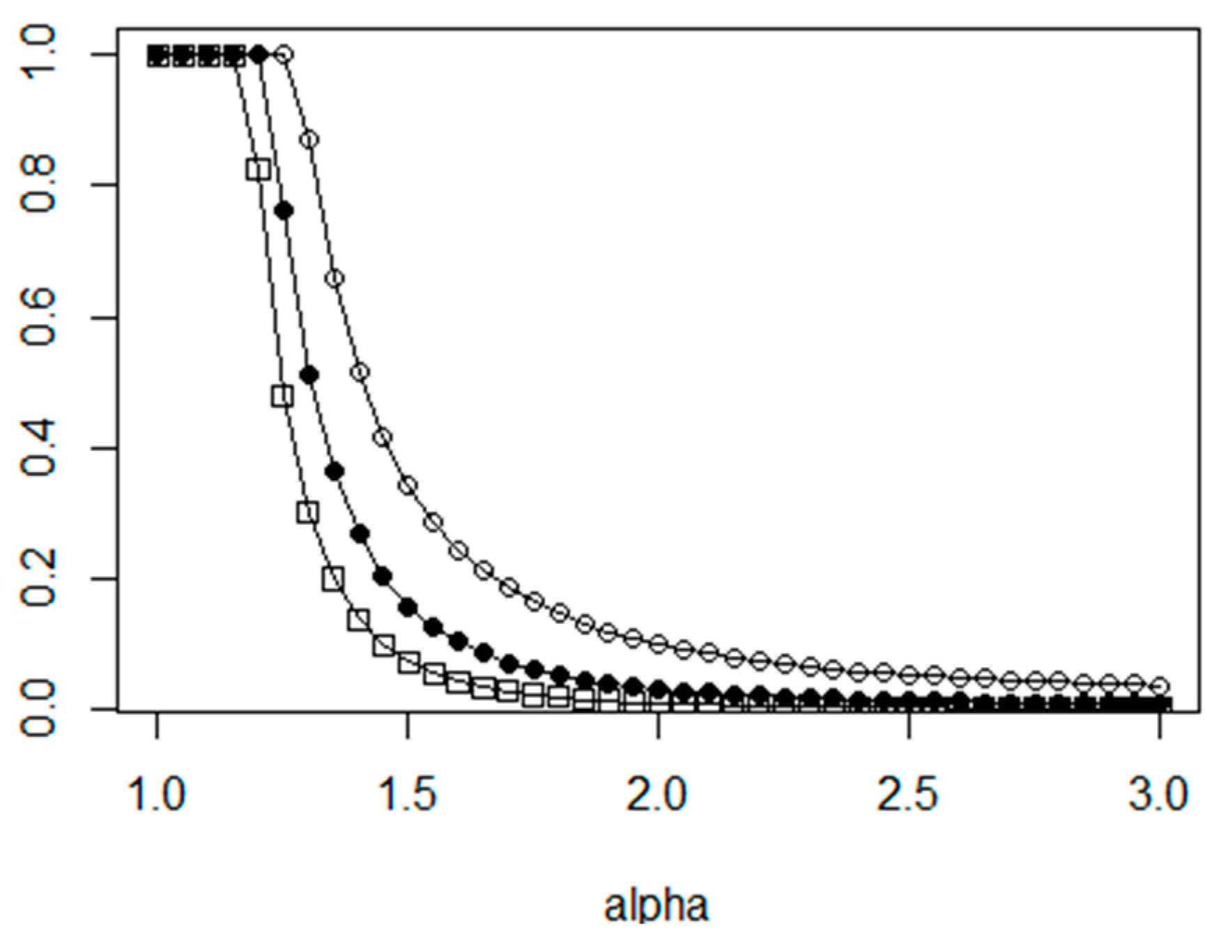
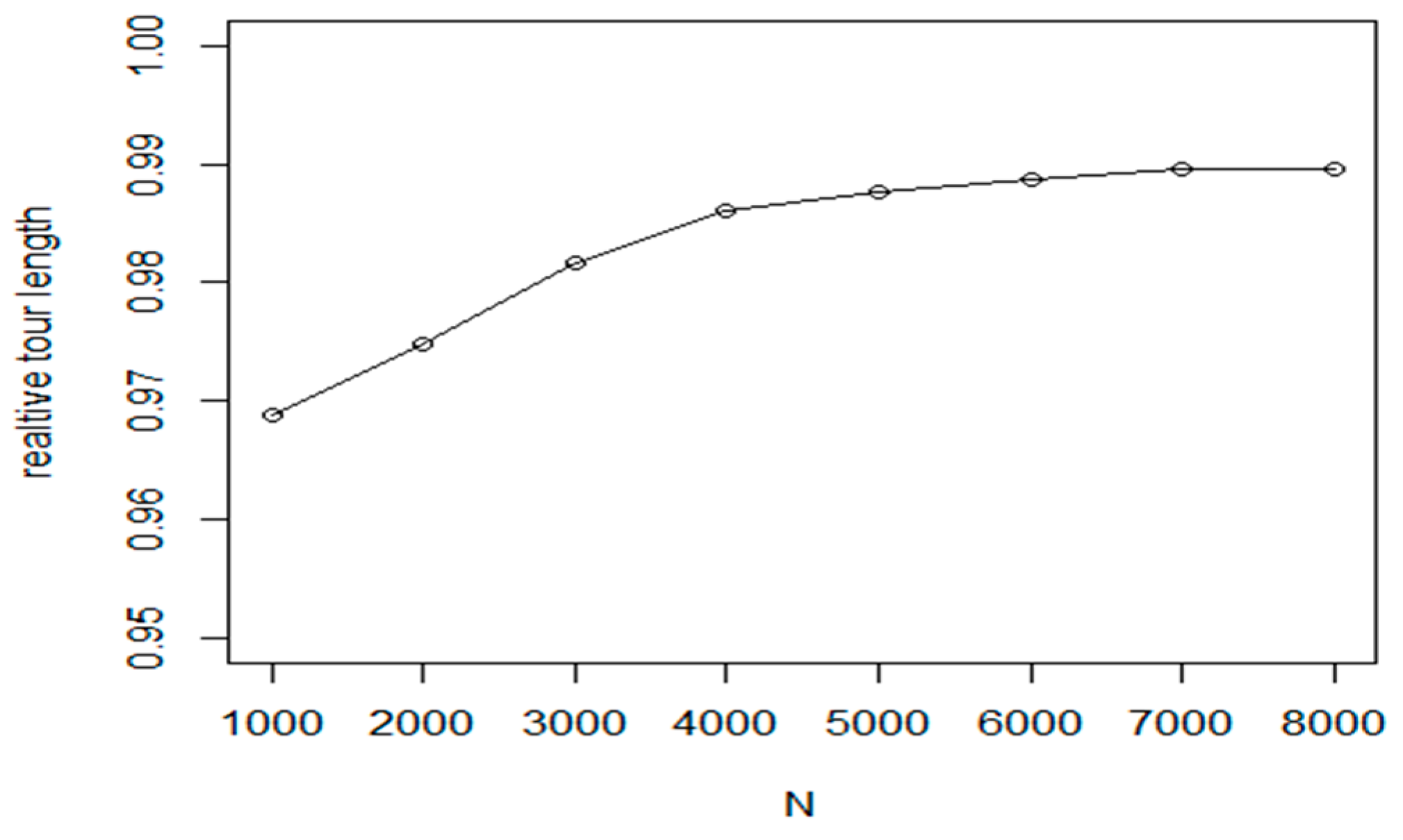
33] of 2.43 for eTSP problems. Regarding the efficiency of the Random insertion algorithm, Azar has proven in Reference [
31] that the worst case approximation factor can be given with
The shape of the worst case factor function is given in
Figure 1.
As this theorem proves the Random insertion method provides in general about 15% weaker result than the Furthest insertion method. In the Random insertion approach, the position of the new node within the route is calculated with a local optimization step. One option is to minimize the tour length increase:
Another option is to connect the new node to the closest tour element:
and take the neighbour node with shortest distance as the second adjusted node.
One of the first publications on incremental tour generation [
34] is made by T.M. Cronin in 1990. The algorithm ensures optimality as each city is inserted. The author has developed a dynamic programming algorithm which begins with a baseline tour consisting of the outer convex hull of cities and proceeds by adding a city at a time to the interior.
The proposed method is based on the following theoretical result: the shortest tour containing
k cities is a quartic and hyperbolic function of the shortest tour containing (
k − 1) cities. It can be proven that an optimal tour must preserve the order defined on the convex hull of nodes [
35,
36]. In this model, a perturbation is a sub-tour which leads into the interior of the hull through two adjacent hull vertices, to capture nodes which do not lie on the hull. Considering the insertion a new node into the tour, the tour is extended by inserting the new node between those two nodes for which the distance is smallest. The tests were executed on small examples containing only 127 nodes.
A generalization of the insertion method is presented in Reference [
37] where during the insertion procedure the two neighbouring nodes of the new item are not necessarily consecutive.
As the practical experiences show [
19] the most efficient methods use a mixed approach where a refinement phase is applied on the tour constructed initially. In our investigation, we focus on segment-level refinement optimization. The motivation on segmentation in eTSP is based on the experience that the optimal route usually connects near vertices in the plane. The segmentation generates a set of smaller optimization subproblems to be solved.
This TSP domain was introduced in 1975 by the research paper [
38]. In CTSP (Clustered Traveling Salesman Problem), the salesman must not only visit each city once and only once but a subset (cluster) of these cities must be visited contiguously. The presented method first reduces the weights of every intra-cluster edges. Then, a standard branch and bound optimization is applied to the whole graph. The performed weight reduction ensures that the optimization algorithm will generate the required intra-cluster routes. Later, several new methods were proposed to solve the CTSP problem, like the Langrangian method using spanning tree constructions for the graph optimization [
39].
The cluster-based segmentation can be considered as an integrity constraints but it can be used a tool for reduce the execution costs of the optimization algorithms. The segmentation as a divide and conquer approach was introduced among others in Reference [
40], where the algorithm starts with the segmentation of the nodes into disjoint clusters using a K-means clustering algorithm. In the next phase of the proposed method, the local clusters are optimized using the Lin-Kernighan method yielding a set of optimal local tours. The local tours are merged into a global tour in the final step. In the merge phase, the cluster centroids are calculated first, then
k-nearest elements in the global tour are determined. Next, each of the
k nodes will be tested to determine the cost of inserting the cluster tour in place of the following edge. The given local tour will be inserted before the node with best cost value.
The idea of combining local clustering (segmentation) in generation of initial route is used in many current proposals. In the literature, we can find many variants of this segmentation approach, as Geometric Partitioning [
41], Tour-Based Partitioning [
42] and Karp’s Partitioning Heuristic (Karp) [
43]. In more complex cases, like [
44], the method constructs a hierarchy of segmentations in order to provide a cluster leaves with small amount of graph nodes. In Reference [
17], the graph nodes are separated into four disjoint groups corresponding to the different sides of a rectangle. In Reference [
45], the route generated by merging the cluster level clusters is refined with a genetic algorithm heuristic. In Reference [
46], the genetic algorithm and the ant colony optimization are used to find the optimal local path for the clusters. In the final step, a simple method for choosing clusters and nodes is presented to connect all clusters in the TSP. The Tour-merging Method [
27,
35] is based on the observation that the routes of good quality usually share a large set of common edges. The algorithm uses specific heuristics to generate near optimal tours and specific dynamic programming techniques to unify the partial solutions into a common solution.
The extensive literature survey that we made shows that the targeted incremental graph and optimal route construction approach attracted little attention and no detailed analysis can be found. In contrary to the rich variety of optimization algorithms on general TSP, only the Random point insertion method can be used directly as an incremental TSP method. As the Random point insertion method is considered as a sub-optimal algorithm dominated by many other methods (like Furthest point insertion, Chained Lin-Kernighan), our motivation is to propose a novel incremental method having a better optimization efficiency than Random point insertion method has and having a better execution cost than the standard non-incremental TSP methods have.
4. Cost Analysis of the Cluster Level Refinement Method
In the cost analysis of the tour construction algorithm using cluster level refinement (intra-cluster_reordering), the cost factors depend on the following parameters:
N: number of vertices in V;
f: cost function of the local optimization algorithm;
N′: number of vertices in local cluster V′;
In the
partition_tour function, the tour
T is segmented into
V′ inner and
V′ outer sections. Having a list representation of the tour and using a status field in the vertex descriptor, the cost of this step can be approximated with
Regarding the generation of the distance matrix, there are two main approaches to be applied. In the first version, there is a global distance matrix generated in the preparation phase of the optimization algorithm. This step requires
cost, while the other approach does not use a global distance matrix but it calculates the local distance matrix in each iteration step. The cost of this step is equal to
The generation of the local optimum route is performed with a cost value
In the last phase, the local optimum tour is merged with the current global optimum tour. The cost of this operation is equal to
In the case of application of global distance matrix, the total cost can be given with
where
m denotes the total number of iterations. Considering a partitioning with
M clusters, the approximation for the cluster size is
The value of
M related to the optimum cost can be calculated with the following formula for the case of global distance matrix:
When using local distance matrix, the corresponding equation is
Using the approximation
where
The optimal cluster number for the global distance matrix approach is given by
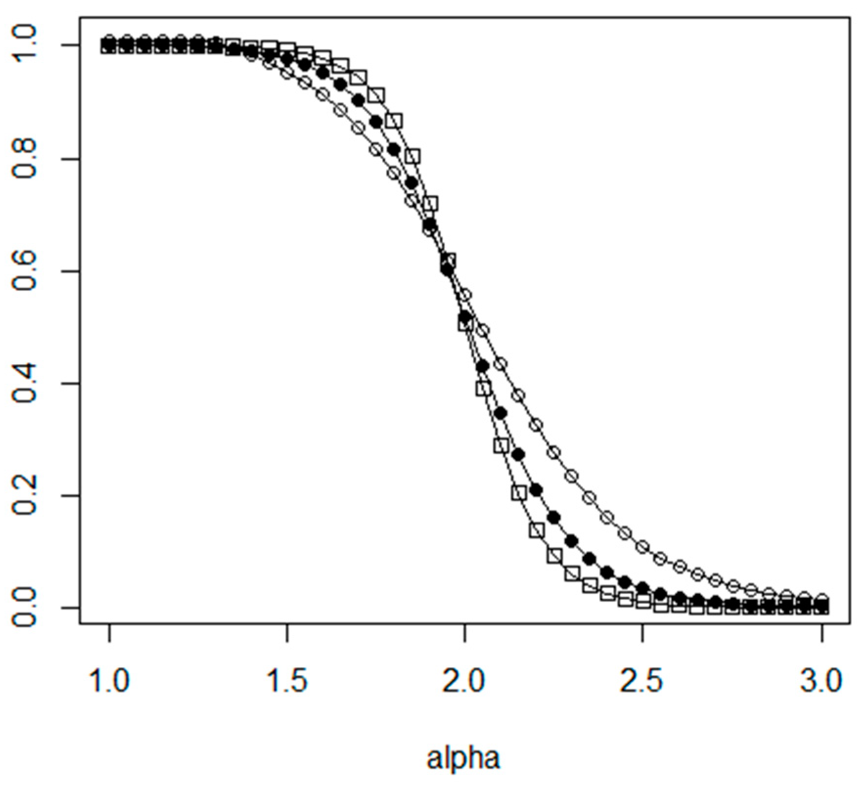
The optimal relative size of the clusters depends on both the α parameter and the N value. Taking the simplification assumption that all the cost coefficients are equal to 1 (
= 1,
= 1, …), we can calculate the optimal values. The dependency between α and the optimal cluster size is shown in
Figure 4, where the curve denoted with hollow circle is for
N = 100, filled circle for
N = 1000 and rectangle symbol is for
N = 10,000.
In the case of local distance matrices, the optimal
value is calculated as the solution of the following equation:
In
Figure 3, the optimal relative size of the clusters is shown for two
N values, the line with hollow circle notation belongs to
N = 100, the line with filled circles relates to
N = 1000. As the figures show, in the case of local distance matrix management, the optimal cluster sizes are smaller than the optimal sizes of global distance matrix management.
Considering the time cost of a global optimization and of the optimization for the partitioning with optimal cluster size, we get the ratio function presented in
Figure 5. The function shows the ratio value
for different α values. Based on the test calculations, we can say that the partitioning method provides benefits especially for larger problems using base optimization method with higher execution costs.
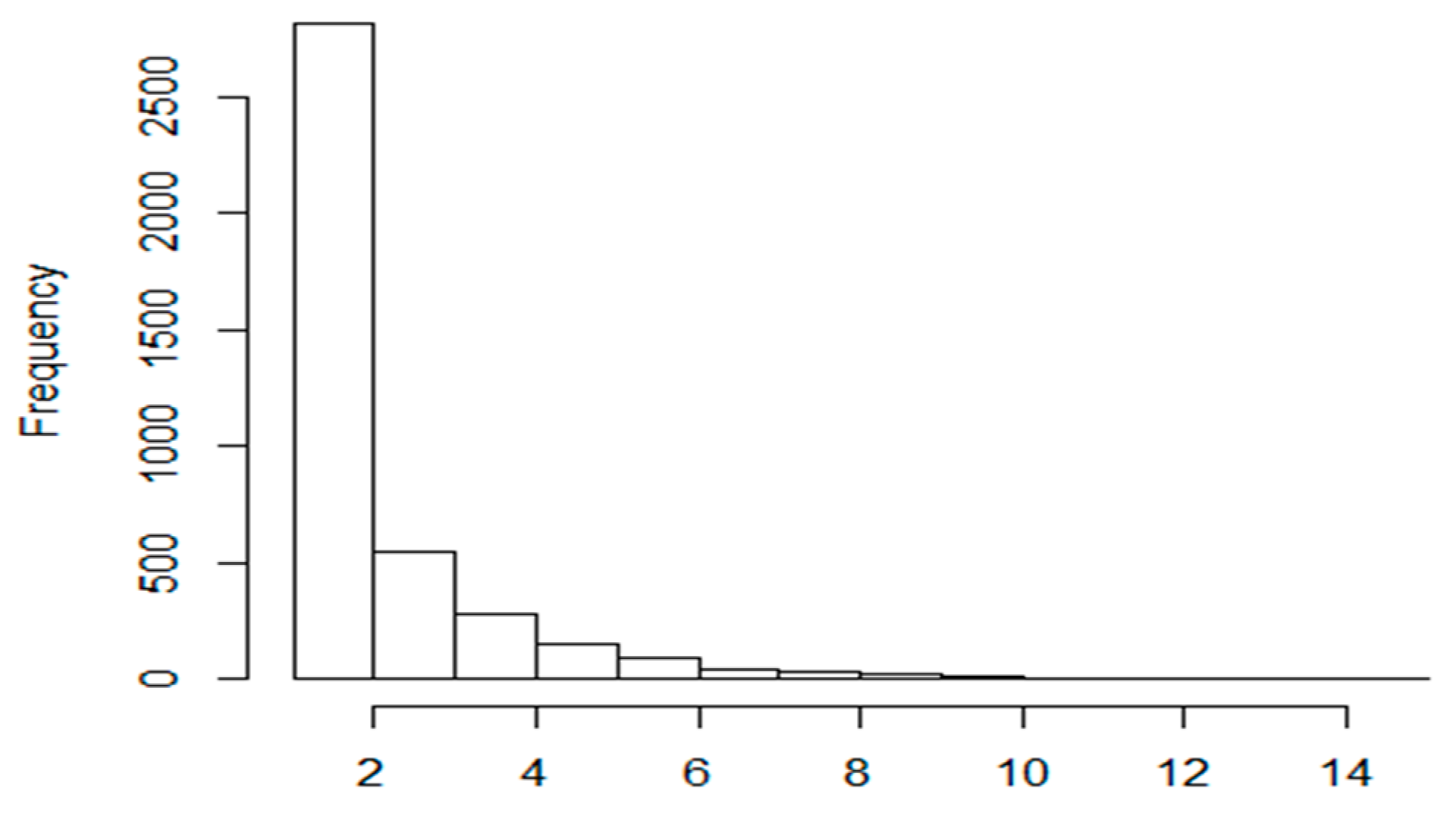
Considering the construction of clusters, there are many different clustering approaches in the literature. In our algorithm, the quality threshold clustering method was implemented as it has many benefits from the viewpoint of the sTSP problem. Based on the obtained experimental results, we can say that the adjacent elements in the route are usually the nearest neighbours in the object space, too. We have investigated optimal tours and tested whether adjacent elements of the route are nearest neighbours in the node space or not. In
Figure 6, the histogram of the adjacent element’s position in the corresponding neighbourhood is shown. The axis X denotes the position in the neighbourhood and axis Y denotes the corresponding frequency in the set of adjacent elements. In the test
N is set to 4000. According to our test results, about 75% of the adjacent elements are the nearest neighbour elements, too. Thus the clusters must contain elements which are in the near neighbourhood of each other. The cliques generated by the QTC algorithm can provide this property as it contains such elements that for every pair, the distance is always less than a given threshold:
5. Performance Evaluation Tests for Local Refinements
In the following, the efficiency of the proposed intra-cluster level route improvement approach is investigated. The main question is to what extend can the intra-cluster level reordering improve the shortest tour found so far. For the performance analysis, a series of tests were executed.
Our tests focused on the operations where the proposed cluster level refinement method may provide an improvement against the competitor methods. There are three main areas where IntraClusTSP can be applied to improve the optimization performance:
- (a)
General refinement of initial tour using arbitrary internal/local TSP optimization method;
- (b)
Application of refinement for a specific local area;
- (c)
Incremental route generation.
In the case of incremental route generation, an existing node graph with optimal route is extended with a new node. The task is to generate a new optimal Hamiltonian cycle involving the new node. One solution is to consider the new graph as an independent new task and we use some existing batch TSP optimization method. This solution requires a lot of redundant calculations as most part of the tour remains unchanged. The incremental approach will perform only the required modifications on the initial route, thus its time cost is significantly lower. Among the known TSP optimization method, the NN algorithm is based on this incremental approach but it tests only a limited set of neighbours to find best position of the new node. From this point of view, the IntraClusTSP method can be considered as an improved version of the standard NN optimization method.
Based on the detailed analysis and performance comparison in Reference [
21,
28,
51], the following methods were implemented for route generation in the performance tests: (a) Nearest Neighbour direct construction algorithm (NN); (b) GA-based refinement algorithm (GA); (c) Hierarchical GA-based refinement algorithm (HGA); (d) Nearest insertion algorithm with refinement (N2); and (e) Chained Lin-Kernighan refinement algorithm (LK).
5.1. Evaluation Methodology
We have selected two different node distributions to generate the input data set for the investigated eTSP problem. The first version is the usual uniform data set distribution in the two dimensional Euclidean space. Most of the benchmark data sets in the well-known TSPLIB library (
https://www.iwr.uni-heidelberg.de/groups/comopt/software/TSPLIB95) have similar distribution characteristics. In this case, the point locations are distributed within a two-dimensional square uniformly. The only input parameter of the input set is the number of points (N). The second distribution model uses two level distribution, that is, there is cluster level containing the cluster centres and there is node level distribution for the point positions within the clusters. The elements of both levels are generated with uniform random distribution. Here, the generation algorithm involves the following parameters: number of the clusters (
M), number of the points (
N), radius of the clusters (
).
In the tests, one execution step corresponds to a series of local refinement runs on all elements of a partitioning. For example, if the domain is partitioned into M clusters, the execution step contains M runs on all of the clusters. In the experiments, we have tested clustering with both non-overlapping and overlapping clusters. The cluster shapes considered were circular with a given centroid and radius. In the tests, a clustering is given with the following parameters. N: number of objects, positions; M: number of clusters; : relative radius of the cluster; L: number of iterations.
Regarding the cluster construction for the refinement runs, we have used a QTC algorithm to select a compact set of neighbouring positions. The mean value for the radius of the refinement clusters was set to 15% of the diameter of the base region.
All performance tests were performed in R environment. The Concorde TSP Solver package (
http://www.math.uwaterloo.ca/tsp/concorde.html) was used to execute the Chained Lin-Kernighan algorithm. Using this optimization method, we The Nearest insertion algorithm with two_opt refinement was included from the TSP package. For execution of the GA optimization, the implementation of the GA package was invoked into our test program. In the tests, we have selected the method “linkern” for Chained Lin-Kernighan. Based on our experiments which are summarized in
Table 1, this method provides the best optimization quality. In the table, TL denotes the tour length value, while T is the symbol for the execution time. Three Lin-Kerninghan variants were compared, beside linkern-variant, also the nearest insertion and the arbitrary insertion variants were tested. The Nearest Neighbour and the Hierarchical GA-based refinement algorithm were implemented directly.
5.2. Nearest Neighbour Direct Construction Algorithm
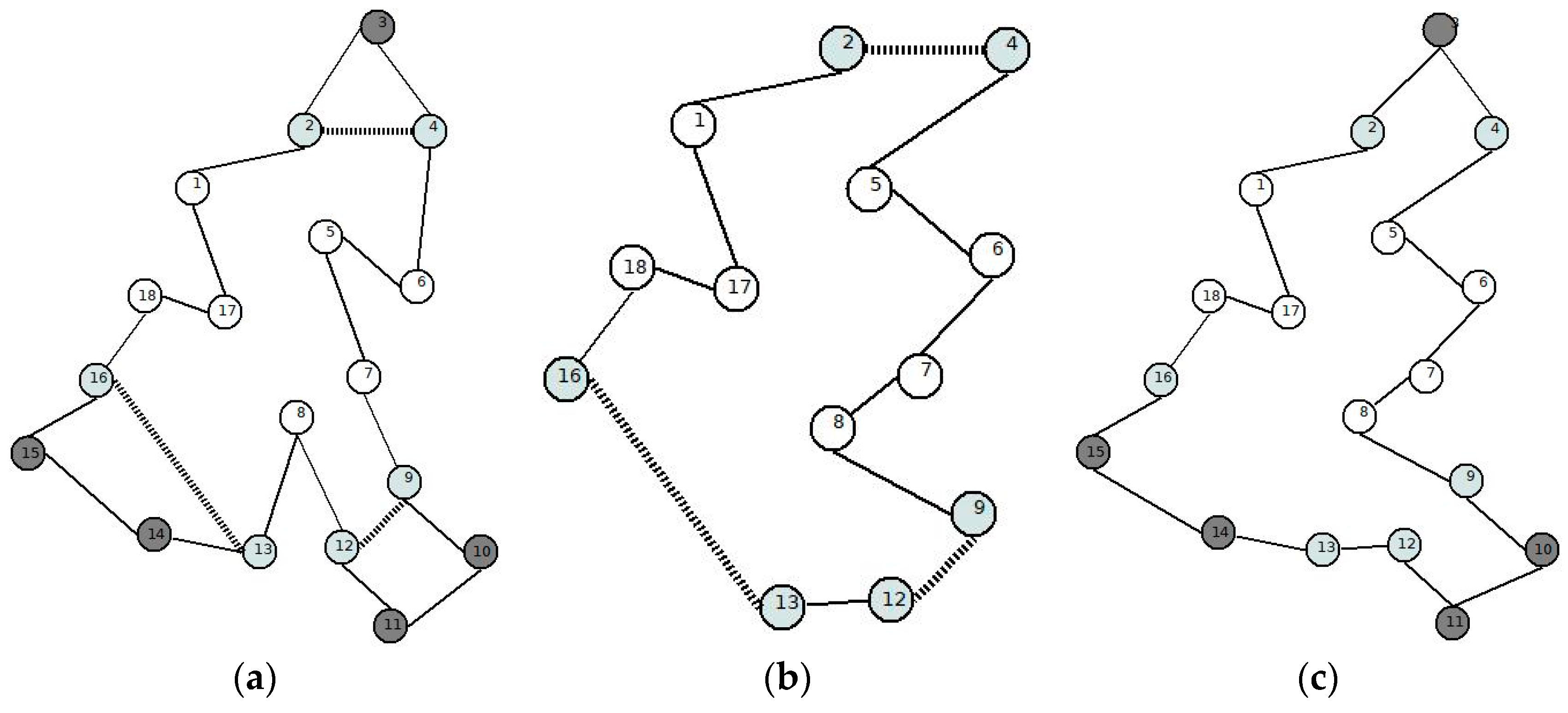
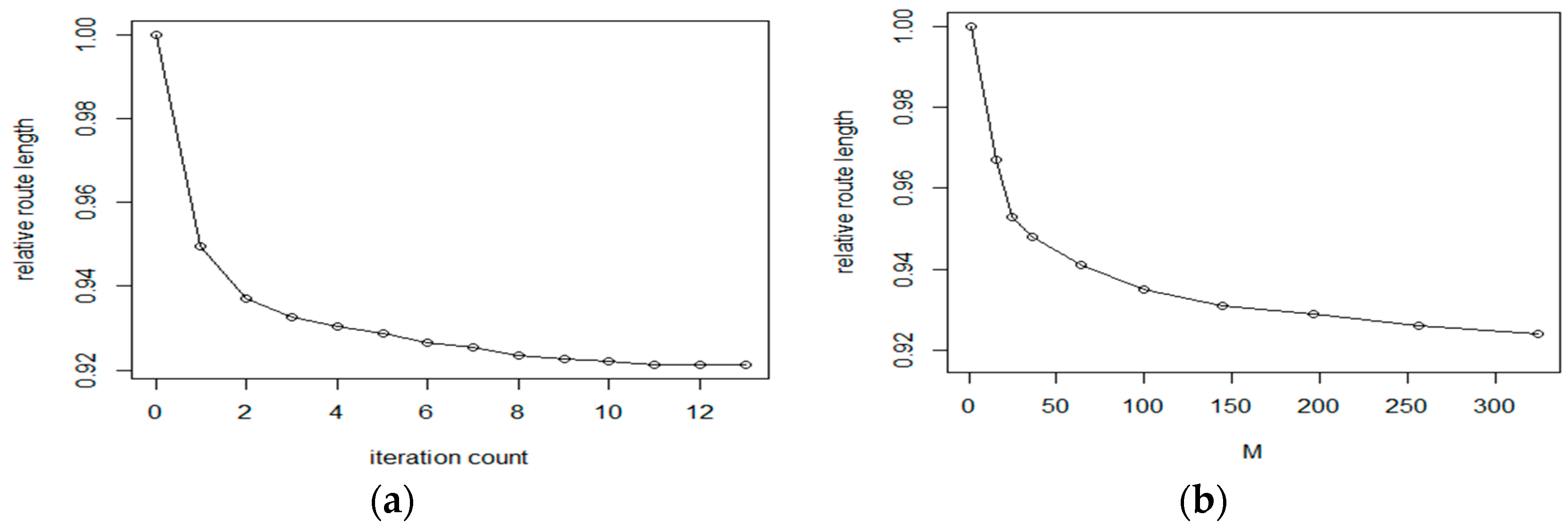
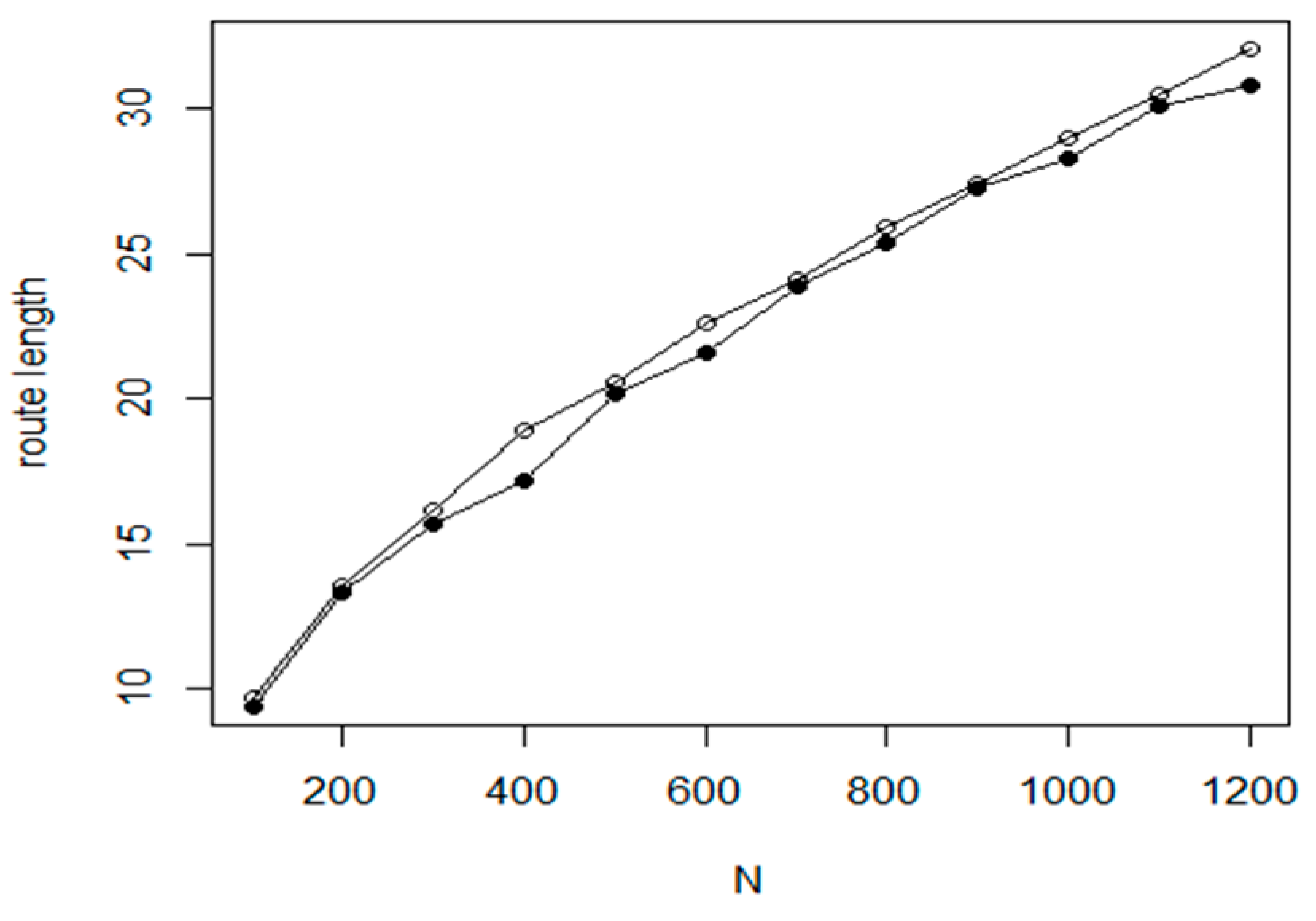
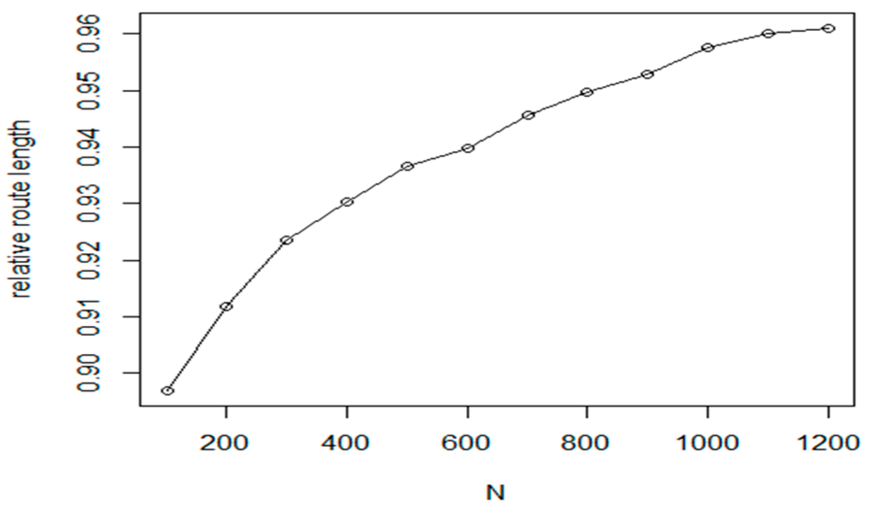
The goal of the first experiments was to evaluate the efficiency of IntraClusTSP refinement algorithm for routes generated by the Nearest Neighbour method. The Nearest Neighbour direct construction method has only one main algorithmic parameter, the distance matrix of the graph. In our case, we have constructed the distance matrix from a point distribution using the Euclidean distance. In the test, we have generated the initial route with the NN method, then we have applied a sequence of IntraClusTSP refinement steps. The results for the data set parameters
M = 324,
= 0.15 on a sample with
N = 6000 are shown in
Figure 7a,b. According to the test results, the proposed cluster route refinement algorithm improved the route length by 8%. As it is shown in the figure, the first refinement cycle provides the largest improvement (about 5%). Based on the literature, the tour length generated by the NN algorithm is about 25% above the theoretical optimum value, the result of the proposed refinement is about 14% above the theoretical optimum. Considering the comparisons performed in Reference [
29], this result is a significant improvement of the original method. The optimal route length as a function of the iteration count is shown in
Figure 4. Considering the number of generated clusters,
M, we can see that the IntraClusTSP method provides a better improvement for partitioning with higher number of clusters.
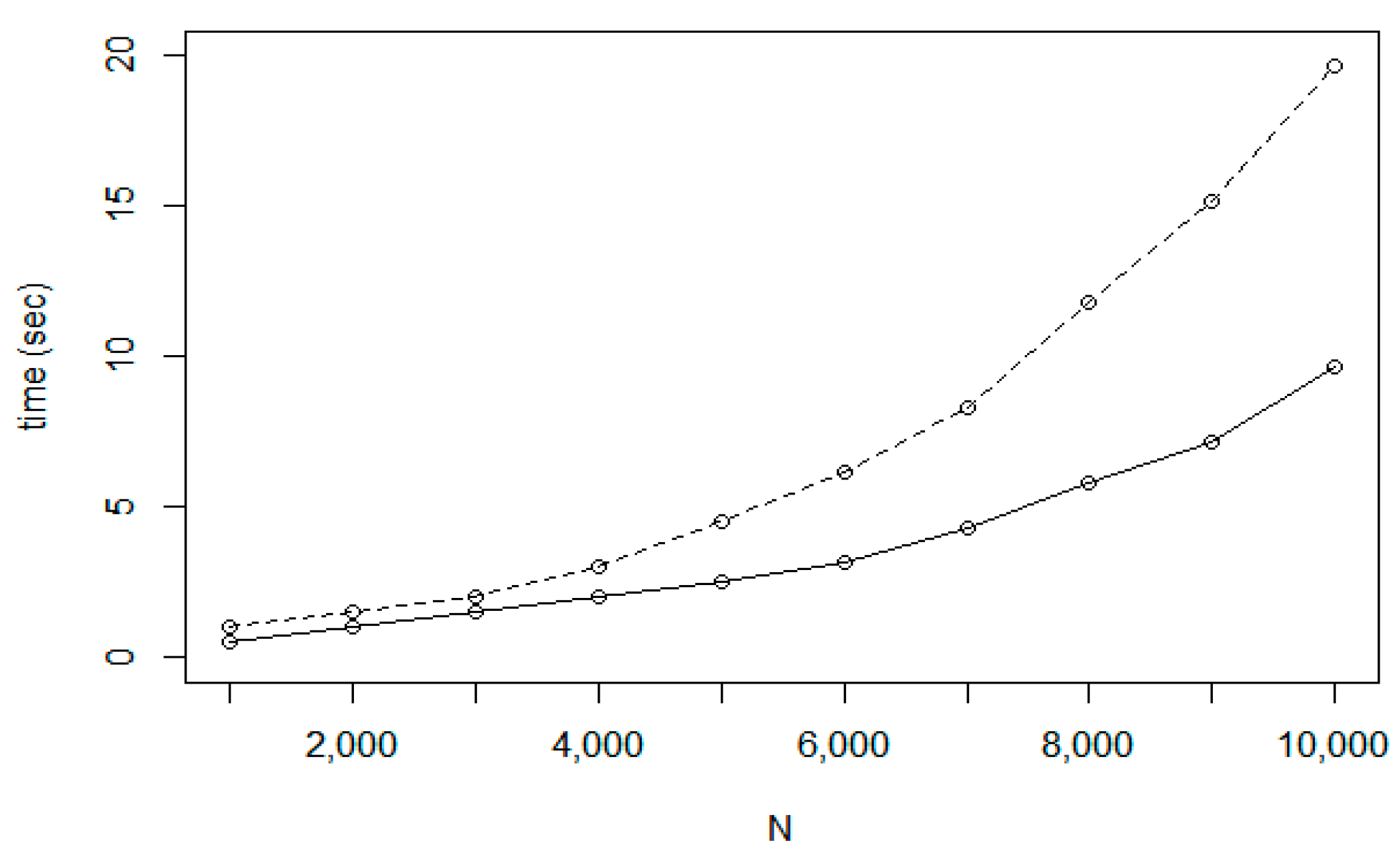
In
Figure 8, two time cost functions are presented. The first function corresponds to the base NN method (denoted by hollow circles) while the second shows the execution cost of IntraClusTSP (filled circle). The second function corresponds to the case when M is equal to the calculated optimum value. As it is expected, the total cost of optimizing the whole node set is higher than the cost to perform a set of local optimizations for the covering cluster set.
5.3. GA and Hierarchical GA Refinement Algorithms
In the GA based refinement algorithm, an individual route corresponds to a permutation of the positions. The fitness of an individual is given with the corresponding tour length. The GA algorithm uses the crossover, mutation and selection operators on the population of selected individuals. Based on our experiences, if the number of population iterations is limited, the GA can provide only weaker results, especially for GA with random initialization. In order to improve the search space, the route of the NN direct optimization algorithm is taken as an element of the initial population. In the case of hierarchical GA, the algorithm first performs a partitioning of the original position set into disjoint clusters. In the next step, every cluster is considered as position represented by the centre point and the optimal route on the cluster level is calculated. Then, for every cluster, a local tour optimization is performed and finally the local optimal routes are merged into a global optimal route.
Based on the experiences, as it is shown in
Figure 9, the random GA is significantly dominated by the NN-initialized GA method. In the figure, the values related to the random GA are given with hollow circles, while NN-initialized GA is denoted by filled circles. The GA algorithm is based on the following main parameters: population size, probability of crossover, probability of mutation, maximum number of iterations to run before the GA search is halted and number of consecutive generations without any improvement in the best fitness value before the GA is stopped. Based on our preparation test, the population size has the largest effect on optimization efficiency. For a wide range of N in our input, the optimal population size is near 40, we have used this parameter in our comparison tests. Regarding the other parameters, the following settings was used: probability of mutation: 0.2, probability of crossover: 0.7; maximal number of iterations: 500 and number of runs: 200.
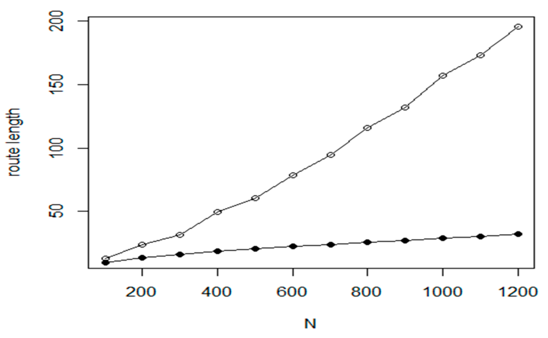
The results of the NN_GA can be improved by some percent using the hierarchical GA approach. The corresponding results are given in
Figure 10, where the filled circles denote the HGA method. The proposed refinement method can reduce the tour length by 5–10%, similar to the base NN approach (see
Figure 11).
5.4. Nearest Insertion Algorithm with Two_Opt Refinement
The Nearest insertion algorithm with two_opt refinement is the default solver in the TSP package of R and it can provide a very good approximation of the optimal route. The Nearest insertion (NI) algorithm chooses city in each step as the city which is nearest to a city on the tour. The NI and two-opt algorithms does not require any special parameter to be set in our tests.
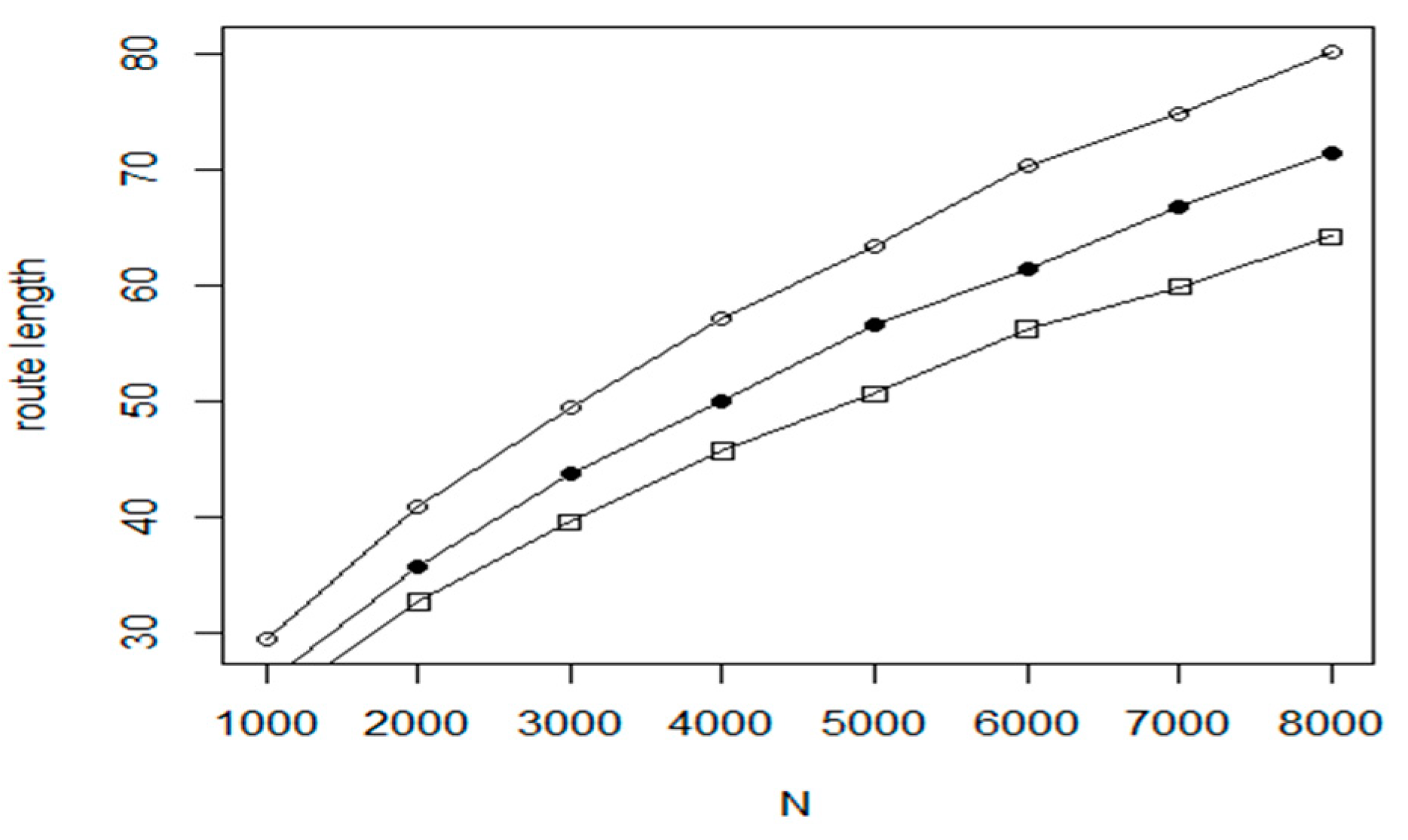
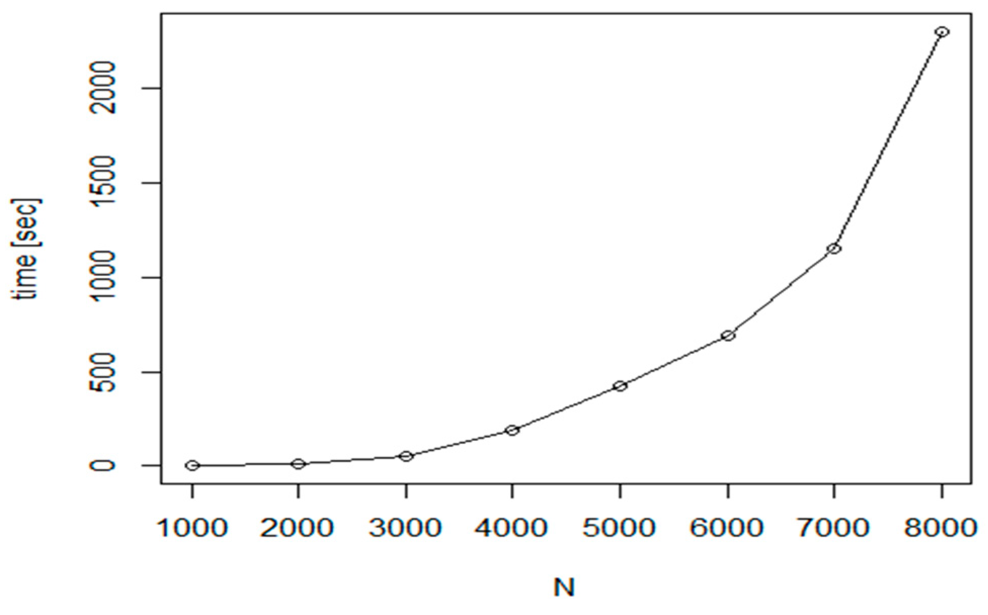
Figure 12 shows the measured efficiency comparison of the Nearest Neighbour method and the Nearest insertion with two_opt refinement algorithm. In the figure, the following notations are used.
The hollow circle denotes the Nearest Neighbour method, filled circle is for Nearest insertion algorithm with two_opt refinement and hollow rectangle is the symbol for the theoretical optimum. Although the efficiency is very good, we experienced a weakness of this algorithm too, the high execution time. As it is shown in
Figure 13, the execution time for the problem with
N = 8000, the required time is more than 200 times larger with
= 10 s and
= 2300 s.
Based on this experiment, the method is not suitable for larger problems. In order to reduce the execution costs, a hybrid approach was introduced in our tests. The proposed method first uses the fast NN algorithm to create an initial route. Then, in the refinement phase, the Nearest insertion algorithm with two_opt refinement is used for tour optimization at cluster level. Taking an iteration of cluster level execution steps, we have created a fast and efficient algorithm.
The experiments prove that the proposed method can improve the efficiency of base method by 2–3% (see
Figure 14) while the required execution time is only a small fraction of the base execution time (
Figure 15). In the experiments, the following parameter values were used:
M is between 25 and 64;
L: between 6 and 10 and
is equal to 0.15.
5.5. Chained Lin-Kernighan Refinement Algorithm
According to the analyses [
19,
28], the Chained Lin-Kernighan refinement algorithm provides the best solution for the TSP optimization problems. Its tour length efficiency is very near to the theoretical optimum (the difference is only 1–2%). This superior efficiency is confirmed by our test experiments too. In our tests, the LINKERN package was used to run the Chained Lin-Kernighan refinement algorithm. The Chained Lin-Kernighan refinement method is an algorithm with many parameters. In our tests, we have used the standard settings [
52] with the following values: Kick value: random walk; number of kicks: number of nodes; method to generate staring cycle: QBoruvka.
The cluster level refinement method can provide here only a tiny improvement. Based on our test experiments, the average improvement ratio is 0.2%, the best result is a one percent improvement for an input distribution with N = 60,000. Considering the fact that the result of the Chained Lin-Kernighan refinement method is very near (1–2%) to the theoretical optimum, the case with 1% improvement is an important achievement.
5.6. Convergence of the IntraClusTSP Refinement Method
In the tests to analyse the convergence of the proposed IntraClusTSP method, we have selected the GA method with random initialization to generate the initial route. Regarding the convergence efficiency of IntraClusTSP, the main determining factor is the applied algorithm for the cluster-level optimization. The Chained Lin-Kernighan method applied in our proposal, provides a very fast convergence. In Reference [
53], the investigation of the route length—iteration step function has shown that in the first 20% of the total running time, the optimization process provides 80% improvement and the rest 80% of the time yields 20% improvement. In our cluster-level refinement approach, the convergence rate is influenced by the following factors:
- -
size of the cluster (large clusters can provide larger improvements but they require larger execution time)
- -
quality of the cluster-level route (the quality shows how far is the length of the current route from the optimal length)
As the average quality of the graph increases during the refinement process, the convergence rate will decrease as it is shown also in the referenced paper.
In our convergence tests, we have used random cluster selection. In every iteration step, only one cluster was processed. In the tests, the following parameter settings were used:
N (number of nodes): 400, 800, 1200
r (relative radius of the clusters): 0.1, 0.2, 0.3
m (number of iteration steps): 25
Our test results can be summarized in the following points:
- -
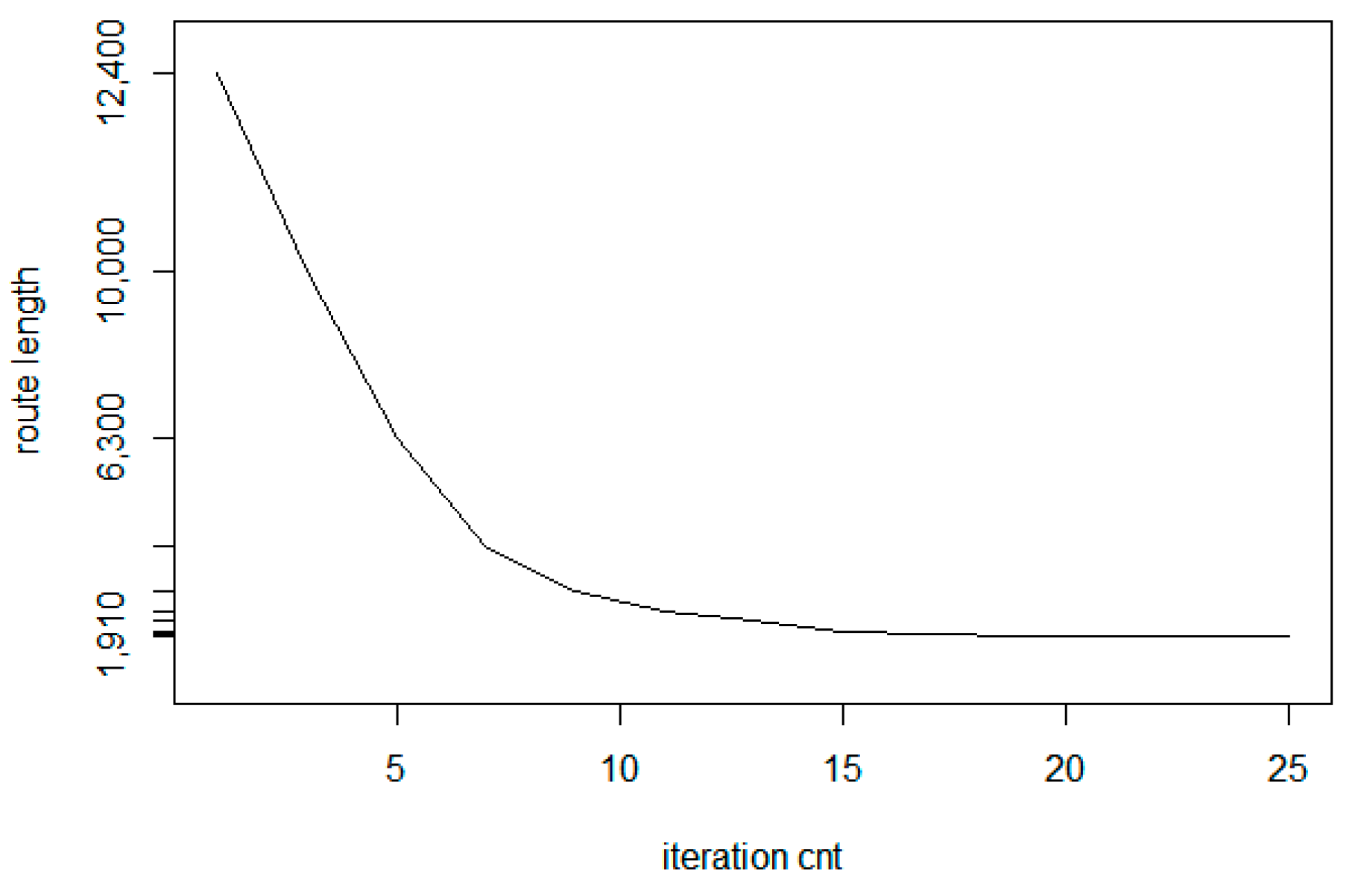
Similar to the convergence of the base LK method, the convergence ratio is significantly larger in the first few iteration steps. In
Figure 16, a sample convergence example is presented as a route length—iteration count function for the input parameters (
N = 400,
r = 0.2)
- -
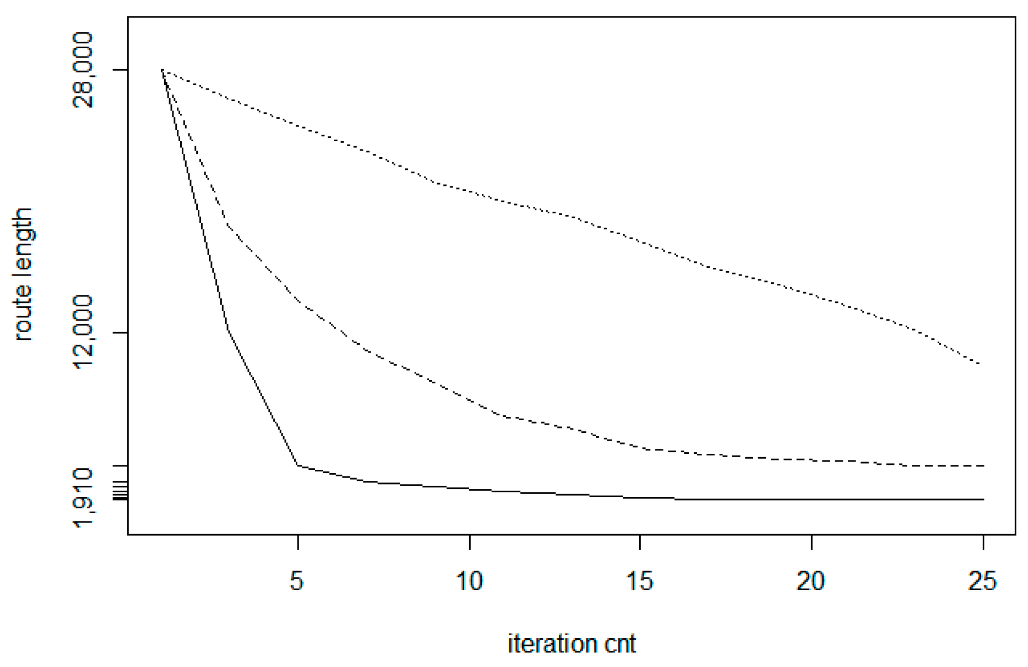
The convergence ratio is larger for larger cluster sizes.
Figure 17 shows the comparison run for three different cluster size values. The bottom (solid) line belongs to
r = 0.3 (large clusters); the middle (dashed) line relates to
r = 0.2 and the top (dotted) line belongs to
r = 0.1. The reason of the fact that the curves may have local plateau is that the clusters are selected here randomly, thus there is a chance to select areas already processed before. In this case, only little improvement can be achieved.
- -
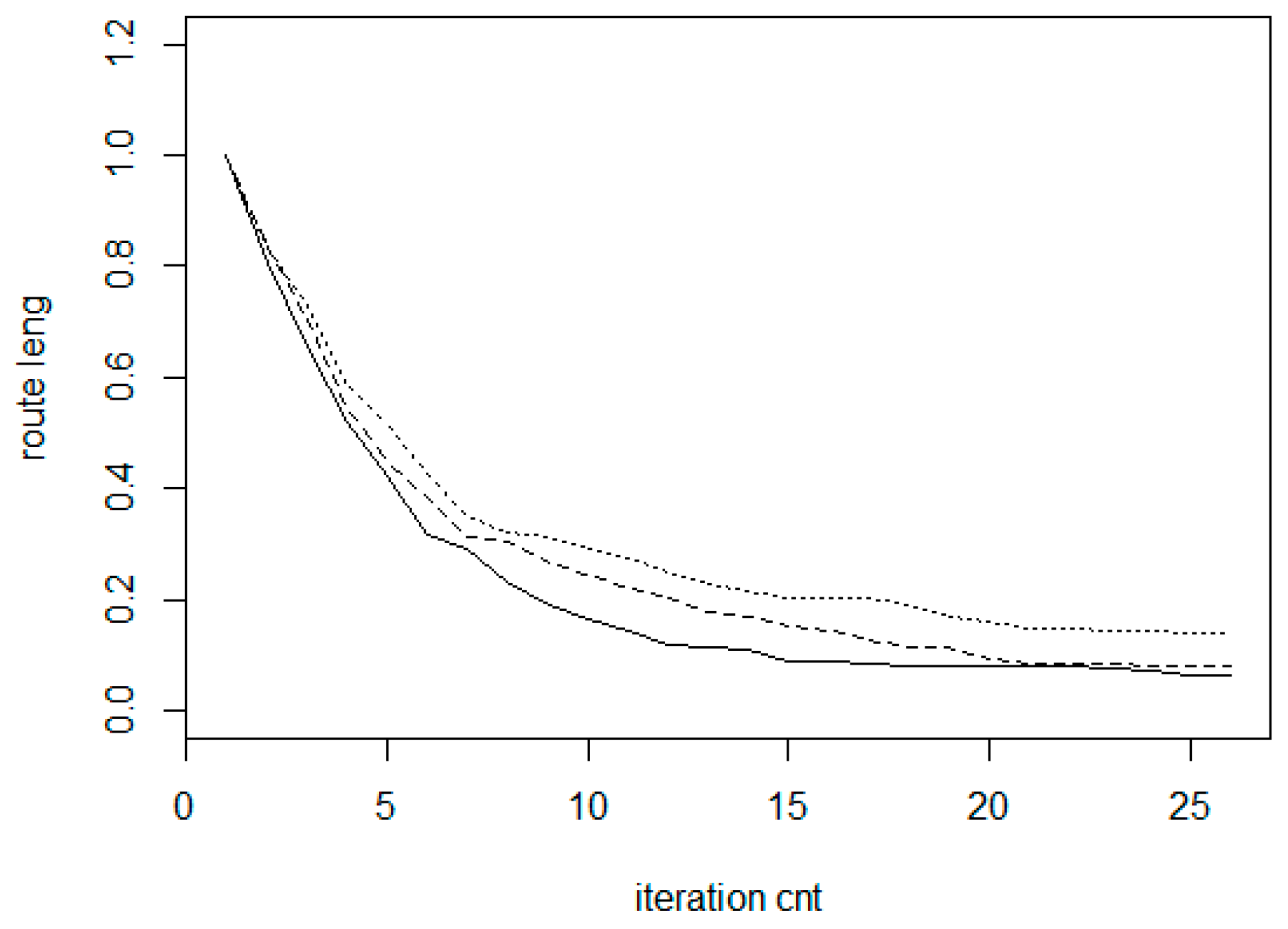
The convergence as relative length reduction is not very sensitive to the graph size but as the experiments show, in larger graphs we can achieve larger length reduction and a better convergence. In
Figure 18, the results for three different sizes are summarized. The bottom (solid) line belongs to
N = 1200 (large graph); the middle (dashed) line relates to
N = 800 and the top (dotted) line belongs to
N = 400.
6. Performance Evaluation Tests for Incremental TSP
In the following, we compare IntraClusTSP with Chained Lin-Kernighan method and with the Random insertion methods from the viewpoint of both time cost and route length optimization efficiency. We have involved the following algorithms into the tests:
- -
Random insertion with random position (RR);
- -
Random insertion with smallest single distance (RS);
- -
Random insertion with smallest route length increase (RI);
- -
Random insertion with smallest single distance with IntraClusTSP refinement (RCI);
- -
Chained Lin-Kernighan method on the whole graph (LK).
In the case of RR, the position of the new node in the route is selected randomly.
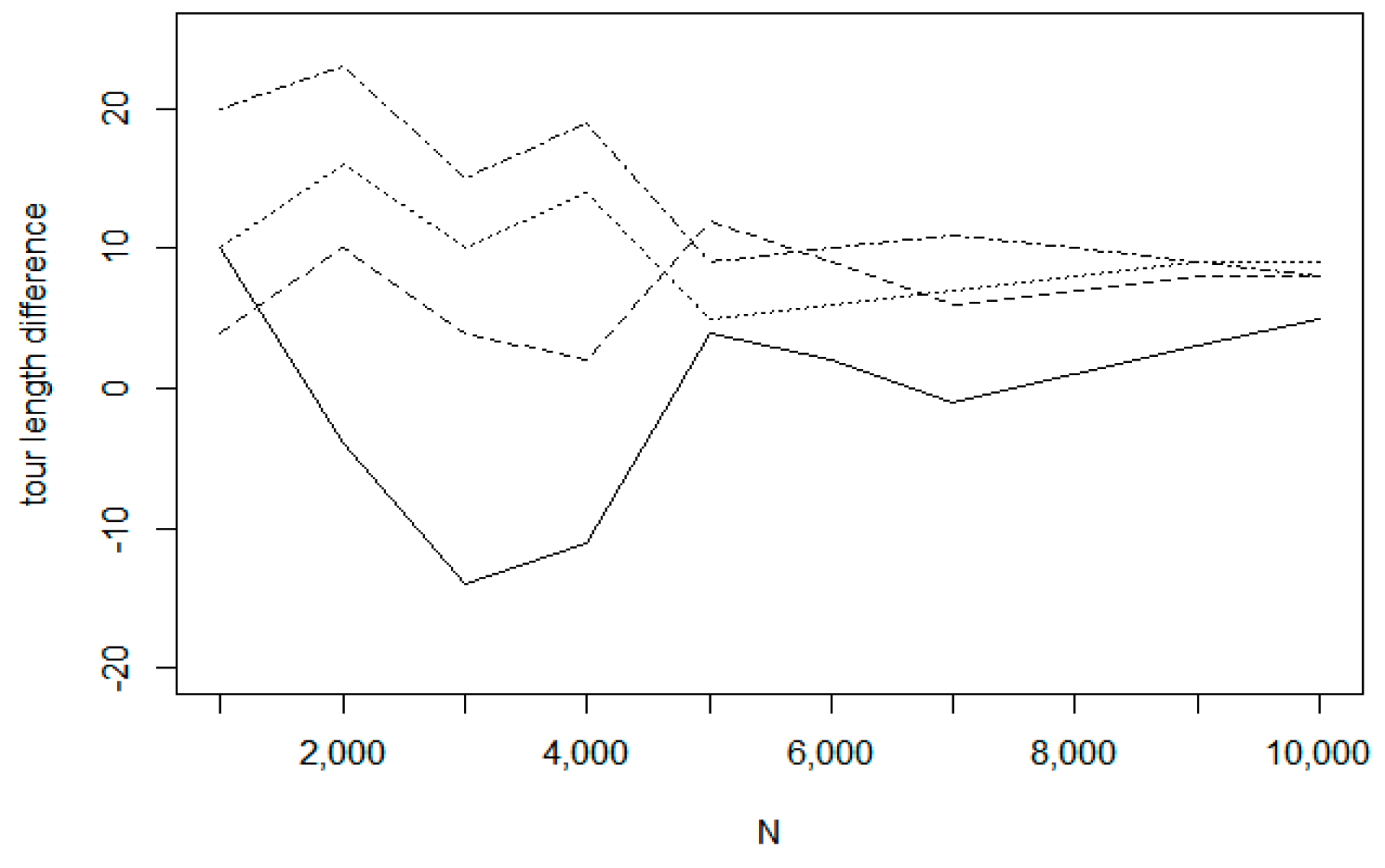
First, we investigate the insertion of a single new node into the current optimal route. Considering the route length optimization, we have experienced that in this simple case, all methods provided about the same result. Thus, there were no significant differences between the investigated methods, only the RR method had a worst time optimization value. In the tests, the method RR provided a very low efficiency as it is shown in
Table 2 and
Figure 19. The input node distribution was generated with uniform distribution within a rectangle area. The size of the graph was running from 1000 to 10,000. The proposed IntraClusTSP algorithm provided a better result than known insertion methods. In
Figure 19 we present the cost difference between the new and old tour versions for the insertion algorithms and for the Chained Lin-Kernighan method. The presented values are the average values related to samples of size 10.
In the next experiments, we investigated the efficiency for insertion sequences, when 200 new elements are inserted into the graph. For the case of single insertion, is proven that our algorithm provides a better result in general but the difference tends to decrease as the size of the initial tour increases. In the case of insertion sequences we may get a different result, as standard insertion methods (RS, RI) can modify only one edge in the original tour, while RCT can perform a larger scale modifications during the same amount of time.
In the tests on insertion sequences, we have selected three kinds of training set. The first is the uniform random distribution (UDT) while the two others (TSPLIB_fin10639 and TSPLIB_xql662) belong to the TSPLIB data repository. For the TSPLIB_fin10369 data set (
http://www.math.uwaterloo.ca/tsp/world/countries.html) we performed two experiments with different initial tour sizes. The test results are shown in
Figure 20,
Figure 21,
Figure 22 and
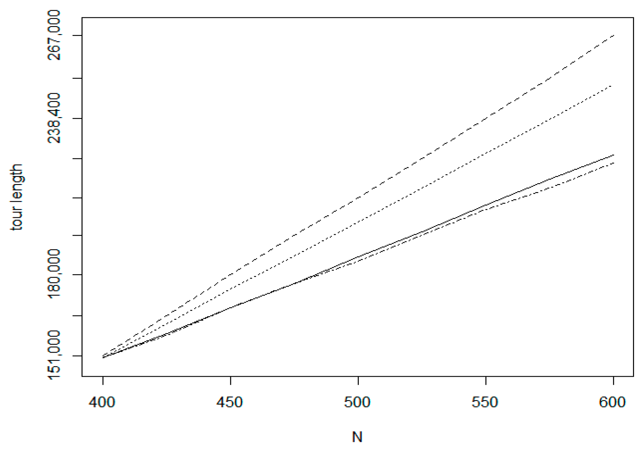
Figure 23. In
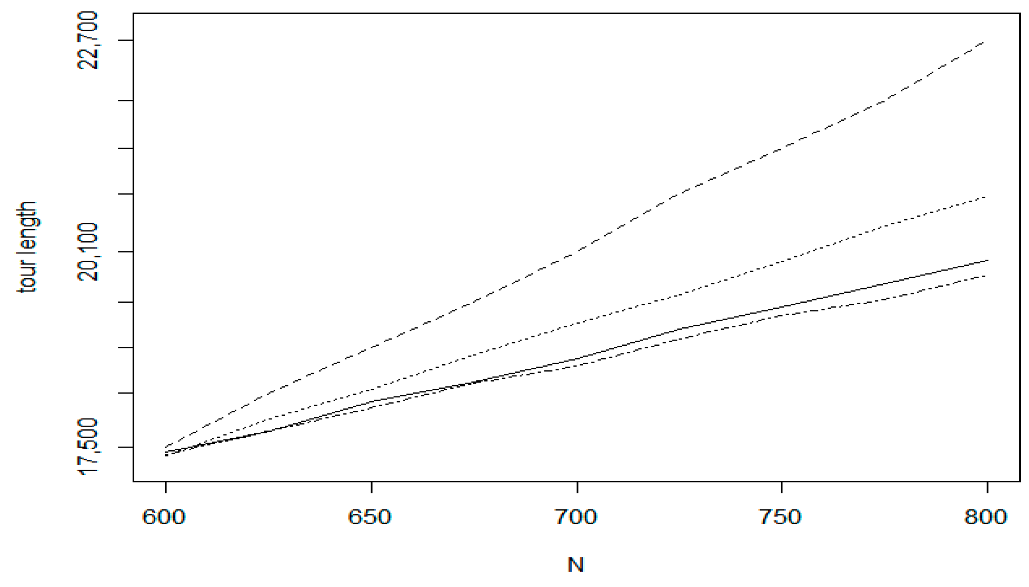
Figure 20 which relates to the uniform random distribution, the bottom dot-dashed line belongs to the Chained Lin-Kernighan method which is a batch method. For this method, the line is a linear approximation, only the values at the start and end positions are measured. For the incremental methods, all values are measurement results. The second solid line denotes the proposed IntraClusTSP method. The next line relates to the RI (Random insertion with smallest route length increase) algorithm and the weakest result is given by the RS (Random insertion with smallest single distance) method. Similar efficiency order can be observed by the other experiments too.
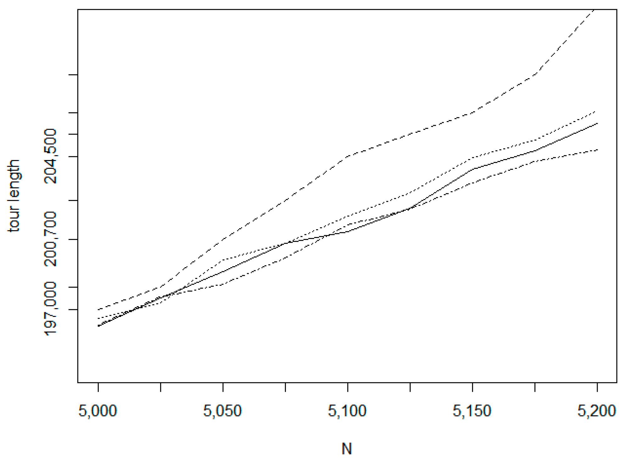
Figure 21 relates to dataset fin10639 on the size interval 5000–5200.
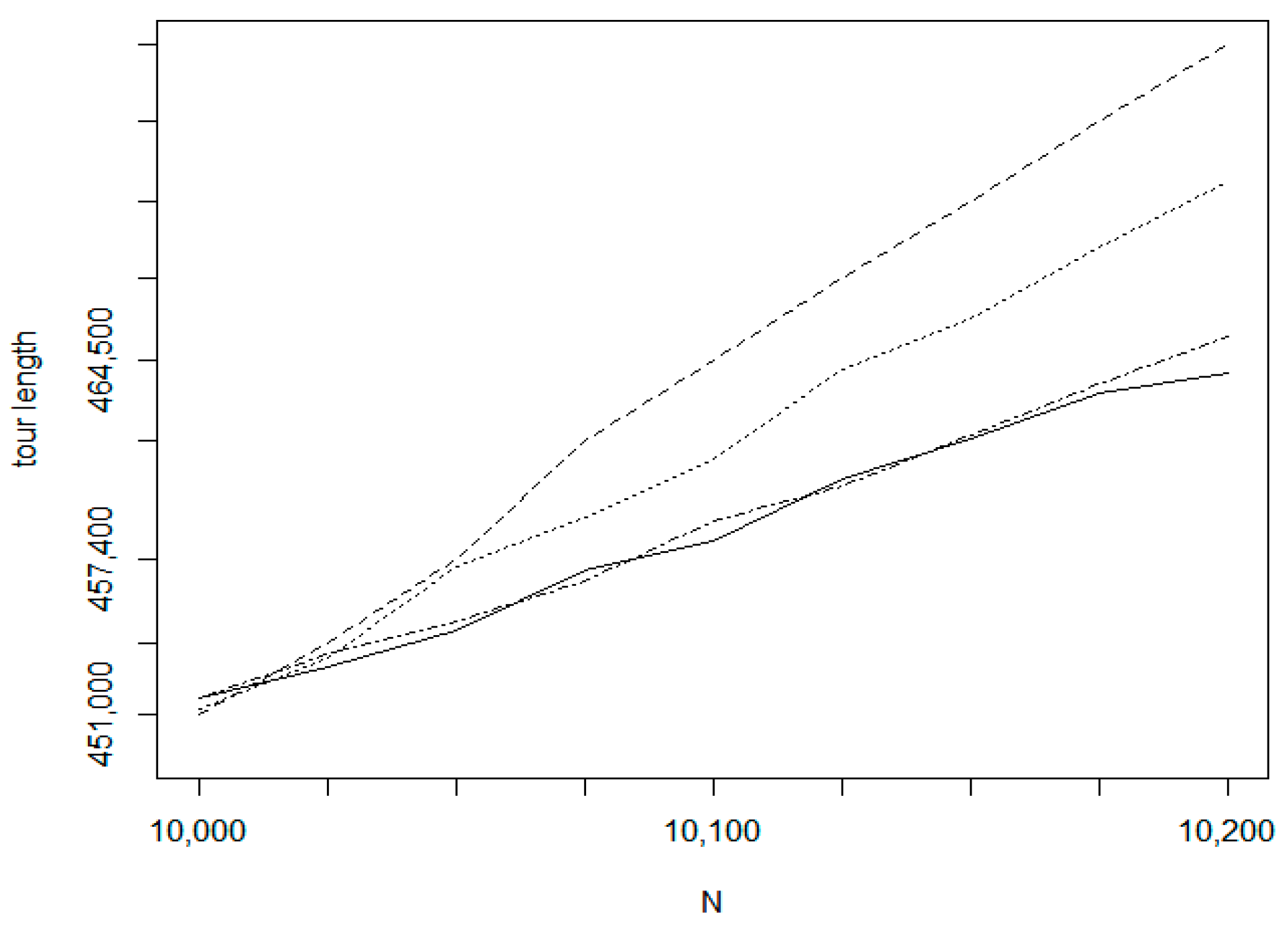
Figure 22 shows the tour length values for the size interval 10,000–10,200 of the same data set. In
Figure 23, the measured tour length values are presented for the TSPLIB xql662 dataset (
http://www.math.uwaterloo.ca/tsp/vlsi/).
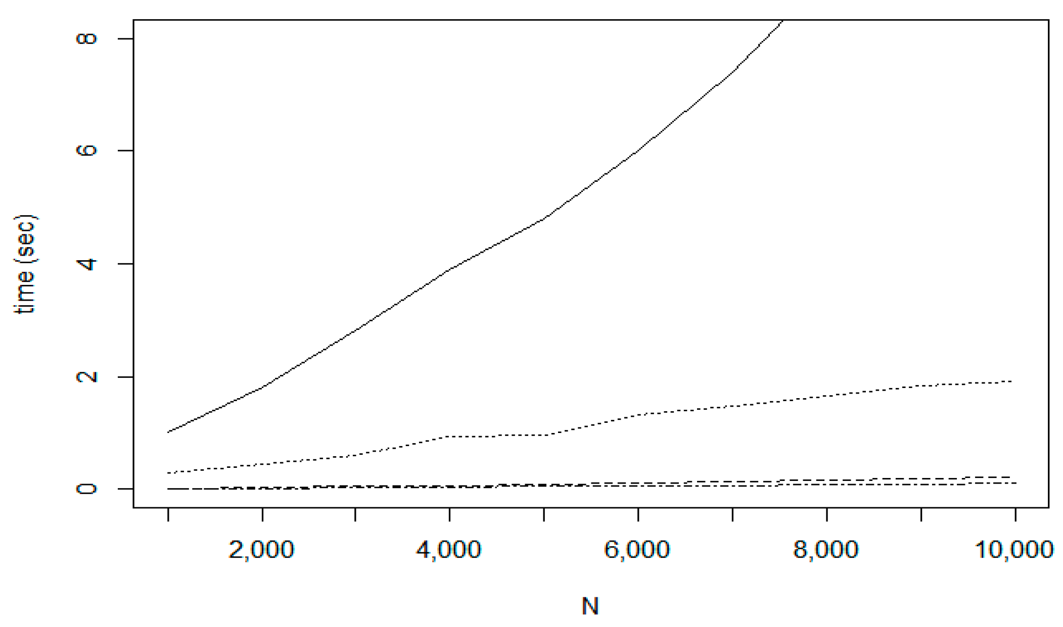
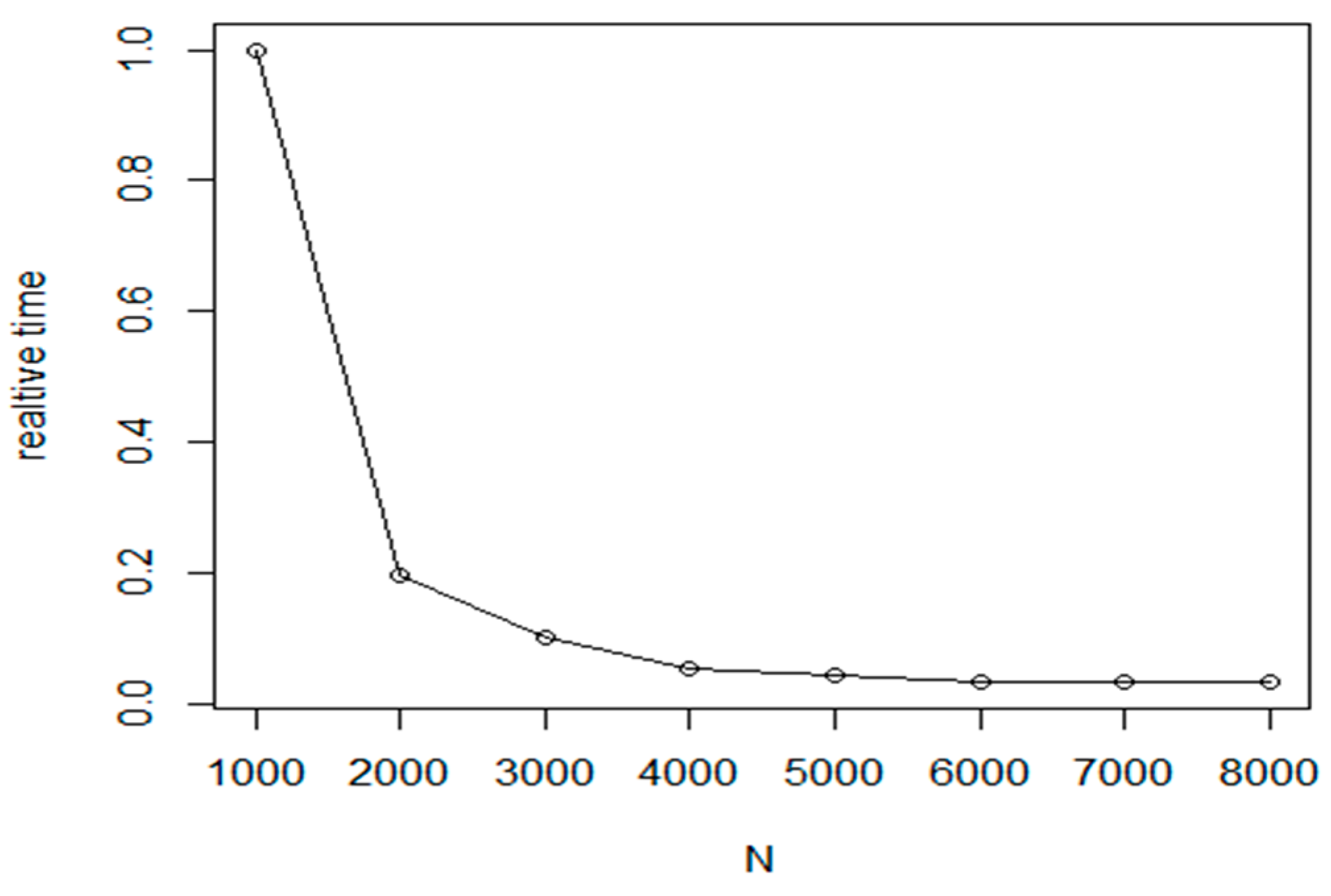
In
Figure 24, the time costs are compared. The largest cost belongs to the Lin-Kernighan method, the cost function of NN shows a very similar characteristics. The incremental route update using the IntraClusTSP algorithm requires only 0.5 s for the graph with
N = 10,000. In case of Random insertion with smallest route length increase algorithm on the fin10369 dataset, required 10 s, which is a significant difference.
The test results proved that the proposed IntraClusTSP significantly dominates the random insertion algorithms on the field of incremental TSP construction, regarding both optimization efficiency and execution costs.
7. Application in Data Mining
The proposed IntraClusTSP algorithm can be used also in the context of data analysis to support clustering A cluster group consists of elements similar to each other. A key factor in clustering is the quality of the clustering (how similar are the objects within a cluster to each other) [
54] and the number of the clusters. Usually, the users should set this number either directly or indirectly in advance as an input parameter of the clustering process. For example, in the case of k-means clustering, the number of required clusters is fixed in advance. The determination of the appropriate number of clusters, is considered as a fundamental and largely unsolved problem [
50]. In the literature, we can find numerus approaches like Silhouette statistics [
55], gap-statistics [
56] or Gaussian-model based approach [
57].
In this section, we present an algorithm based on TSP optimization to support the determination of the optimal number of clusters. The proposed method is based on the following considerations. As it was shown in
Section 3, the shortest path usually connects the elements located in the neighbourhood. Thus, the distances between adjacent elements belonging to the same cluster, should be small. On the other hand, if the adjacent element belongs to different cluster, the distance should have a large value. Thus, a relatively large distance in the optimal route should mean a gap, a connection from a cluster to another cluster. Based on these considerations, we evaluate the distance function between two adjacent elements of the optimal route to determine the clustering structure.
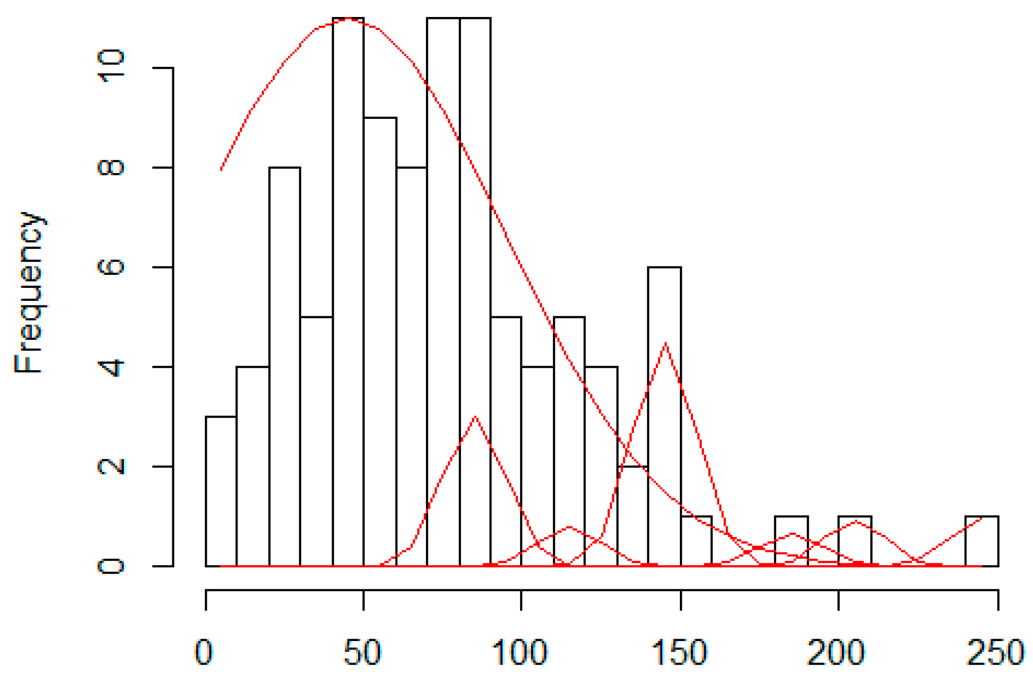
The proposed method is based on the analysis of the corresponding edge length histogram. Having this histogram, we consider it as a mixture of normal distributions and we can perform a Gaussian Mixture Density Decomposition (GMDD) [
58]. In GMDD, having the current density function, we first determine the location of the maximum density and we fit a Gaussian distribution with maximum overlap. This Gaussian is added to the components’ list and this component is removed from the current input distribution. If this reduced density is a not a zero function then it will be analysed in the same way.
Figure 25 shows the result of a sample GMDD process.
Having the GMDD spectrum, we have to determine those components which belong to different clustering levels. In our model, we consider an edge as cluster level connection if its length is significantly larger than the average length of the intra-cluster connections:
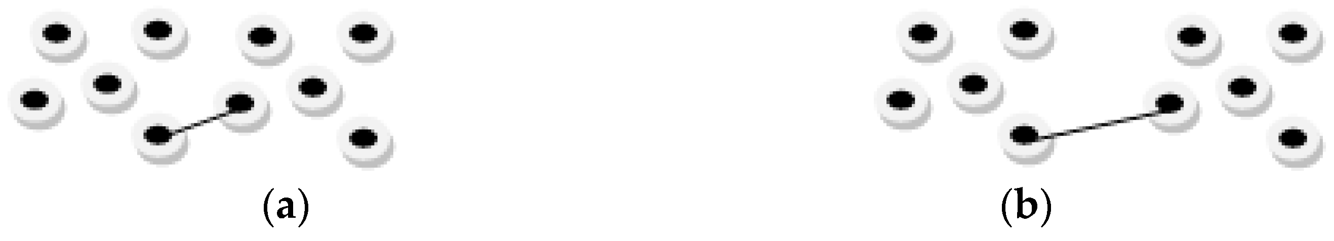
The parameter ∝ is considered as an input parameter of the algorithm. Based on our experiments with human observers, we take value 2 as default value of alpha. Our tests show that the point distribution in
Figure 26a (
) is usually considered as single cluster while the points in
Figure 26b (
) are considered to belong to two clusters.
Thus, if the length difference between two elements in the corresponding edge length histogram is significantly larger than the average length of the previous level, then the larger element will belong to a new clustering level. The algorithm to calculate the cluster counts for different levels can be summarized in the following steps.
| Algorithm 3: Histogram of edge length containing M bins |
| 1: CL := cluster level descriptors; |
| 2: g : = 0; // cluster level index |
| 3: for each i in (1 to M) do |
| 4: b := H[i]; // current bin |
| 5: b.count := count of edges in the bin |
| 6: b.length := average edge length in the bin |
| 7: bp := the previous not empty bin |
| 8: if b.count > 0 then |
| 9: L_g := the average edge length in the current cluster level CL[g]; |
| 10: L_a : = b.length – bp.length; |
| 11: if L_a > alpha * L_l then |
| 12: g = g + 1; //create a new cluster level |
| 13: add b to CL[g]; |
| 14: else |
| 15: add b to CL[g]; |
| 16: end if |
| 17: bp : = b; |
| 18: end if |
| 19: end for |
| 20: Calculate the GMDD distributions for the cluster levels |
In the following, we present the application of the algorithm on an example distribution.
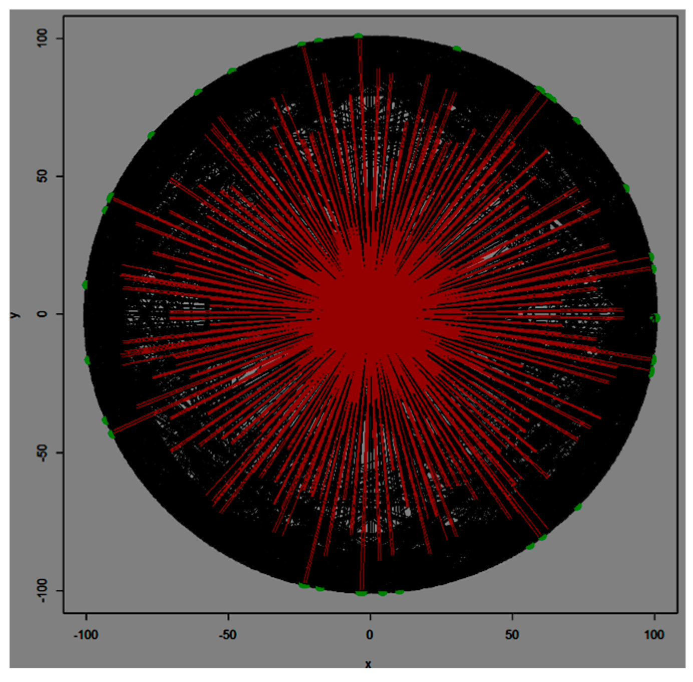
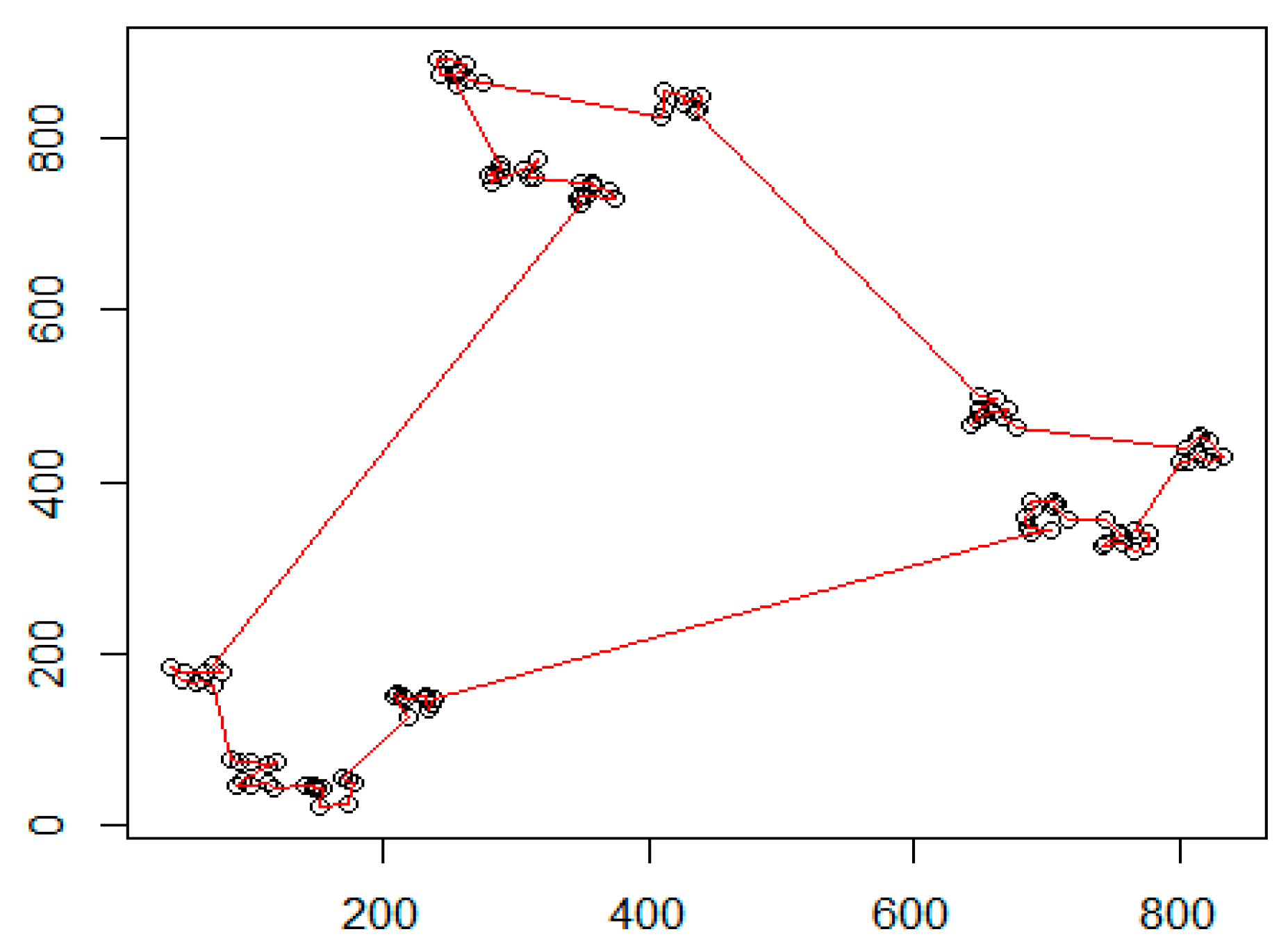
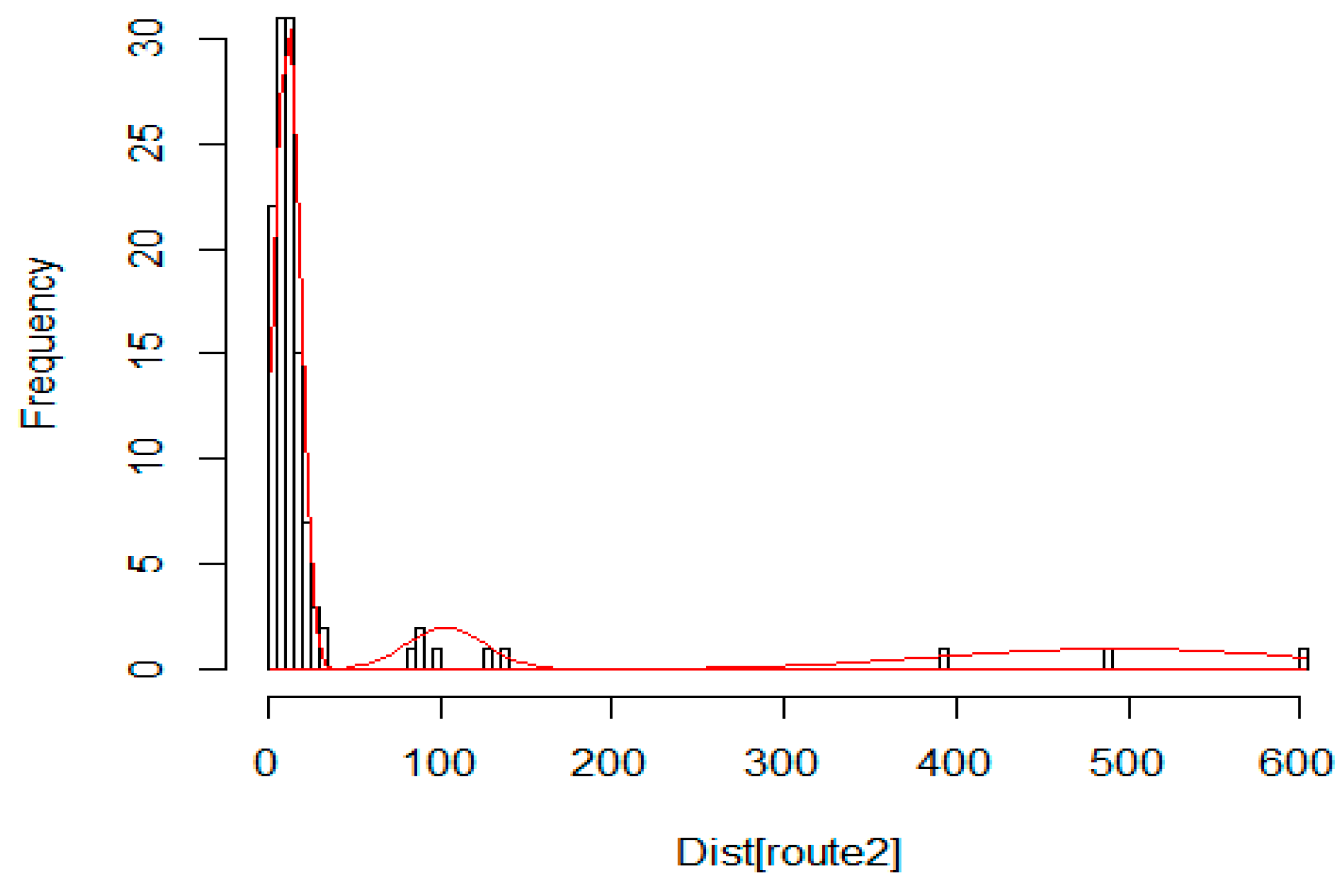
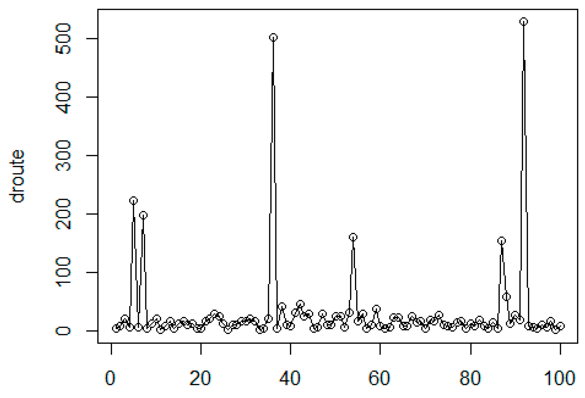
Figure 27 denotes the initial distribution of the graph nodes. Can be detected two clustering levels. At the first level, there are 12 small clusters, while the second level contains three large clusters. The calculated shortest path is denoted by red line. The generated edge length histogram with the GMDD spectrum is presented in
Figure 28, where the corresponding edge-length function is given in
Figure 29. The first large peak belongs to the base level, here we have 120 elements in the distribution. The second peak denotes the first cluster level with the small clusters and the last component relates to the level of the large clusters.
Table 3 summarizes the main parameters of the discovered clusters.
As the results show the method discovered the multi-level clustering structure in the input distribution.
We have compared our algorithm with two widely used methods for determining cluster count. The first investigated method uses the Silhouette index [
59] approach. This index prefers small intra-cluster distances and it is defined in the following way for a partitioning with clusters (
):
The cluster count is the
k value, where the value
is maximum optimum:
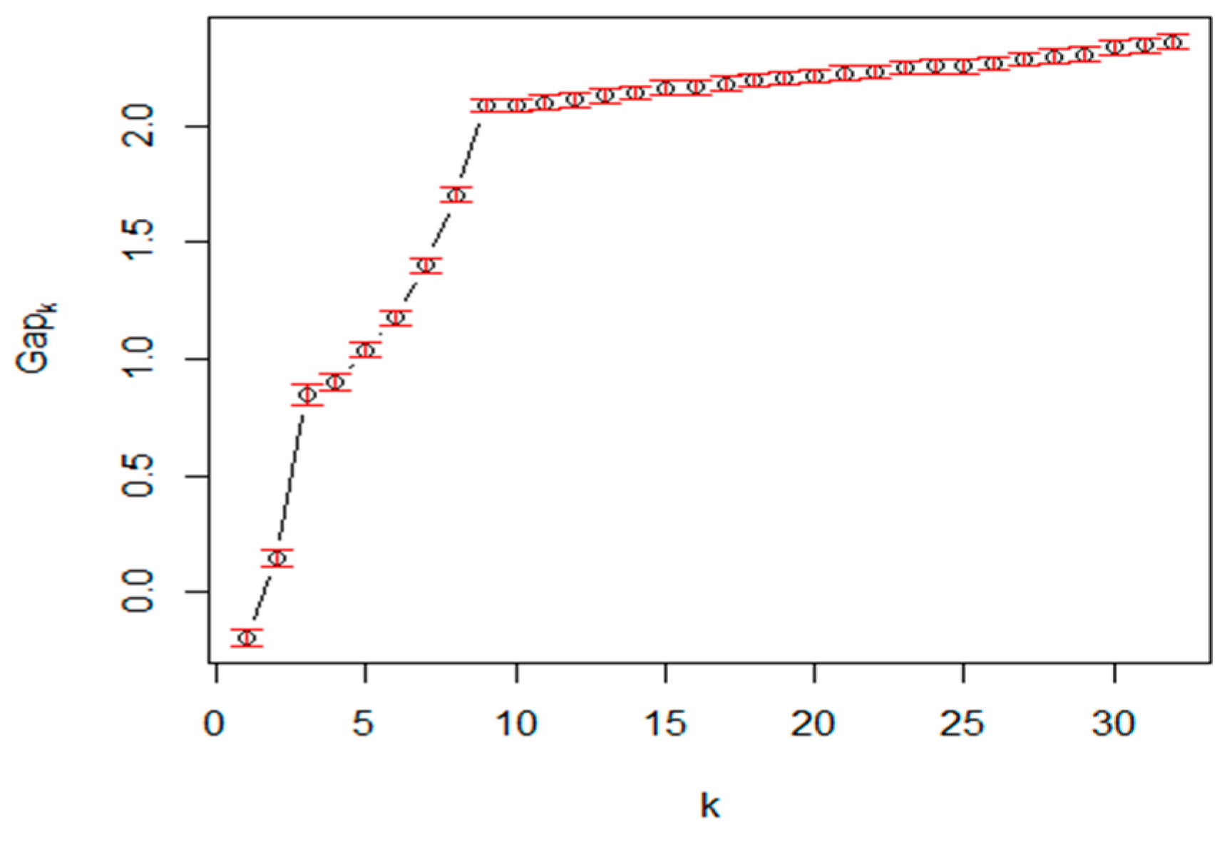
The second investigated method is the gap statistic method [
55] Estimating the number of clusters in a data set via the gap statistics. The method calculates the goodness of clustering measure by the “gap” statistic.
The
value is calculated via bootstrapping, that is, simulating from a reference distribution. A sample calculated gap statistic value in dependency of cluster count
k is shown in
Figure 30. There are different approaches to determine the cluster count
K from the gap function, like the first maximum or the global maximum.
In the comparison tests, the factoextra and cluster packages of R were included to perform the silhouette and gap statistic calculations. In the generated data distributions for the evaluation test, the objects are arranged into either a single-level or a two-level clustering structure. For the comparisons, we have generated
Table 4 describing the typical test results has the following structure:
column (observed): the real clustering structure observed by humans. The column contains one or two numbers. The first number denotes the number of clusters at the first clustering level, while the second value is the cluster counter of the second level.
column (gap-A): cluster count proposed by gap analysis using the first maximum optimum criteria;
column (gap-B): cluster count proposed by gap analysis using the Tibs2001Semax optimum criteria;
column (silhouette): cluster count given by the Silhouette method;
column (multi-level GMDD): cluster count calculated by our proposed multi-level GMDD-based method;
column (time [silhouette]): the execution time of the Silhouette method in milliseconds;
column (time [gap]): the execution time of the gap statistics method in milliseconds;
column (time [ml GMDD]): the execution time of our proposed multi-level GMDD method in milliseconds.
The test results in the comparison of the alternative methods can be summarized in the following experiences:
- -
Only our proposed method can discover the multi-level clustering structure, while the current standard methods are aimed at determining the cluster count of the first clustering level.
- -
In most cases, the proposed method could discover the hidden clustering structure.
- -
Our proposed method could provide the best accuracy in all test cases.
- -
The proposed method requires significantly less execution time.


