Solution of Fractional Differential Equation Systems and Computation of Matrix Mittag–Leffler Functions

Abstract

In this paper, solutions for systems of linear fractional differential equations are considered. For the commensurate order case, solutions in terms of matrix Mittag–Leffler functions were derived by the Picard iterative process. For the incommensurate order case, the system was converted to a commensurate order case by newly introducing unknown functions. Computation of matrix Mittag–Leffler functions was considered using the methods of the Jordan canonical matrix and minimal polynomial or eigenpolynomial, respectively. Finally, numerical examples were solved using the proposed methods.

1. Introduction

In fractional calculus, different possibilities of defining integral and derivative of non-integral order, which generalize the classical integration operator $Jf\left(t\right)={\int }_0^{t}f\left(s\right)ds$ and differentiation operator $Df\left(t\right)=\frac{d}{dt}f\left(t\right)$, are investigated. In this respect, the Grünwald–Letnikov fractional integral and derivative, the Riemann–Liouville fractional integral and derivative and the Liouville–Caputo fractional derivative are commonly used [1,2,3,4,5,6,7].

Fractional calculus has been made use of to model memory phenomena and hereditary properties [2,3,4,5,6,8]. Its application areas have been widely exploited, such as non-Newtonian flow, damping material [4,8,9,10], viscoelasticity theory, anomalous diffusion [11,12,13,14], and control theory [15].

For a function $f\left(t\right)$ defined on $(0,+\infty )$, the Riemann–Liouville integral of order $\beta$ is given as

$$\begin{array}{c}\hfill J_t^{\beta }f\left(t\right)=\frac{1}{\Gamma \left(\beta \right)}{\int }_0^t{(t-\tau )}^{\beta -1}f\left(\tau \right)d\tau \mathrm{for}\beta >0\end{array}$$

(1)

and $J_t^{\beta }f\left(t\right)=f\left(t\right)$ for $\beta =0$, where $\Gamma (·)$ is the Euler’s gamma function. Equation (1) can be expressed as a convolution as

$$\begin{array}{c}\hfill J_t^{\beta }f\left(t\right)=\frac{t^{\beta -1}}{\Gamma \left(\beta \right)}\ast f\left(t\right).\end{array}$$

(2)

The Riemann–Liouville derivative of order $\alpha$ is defined in the form

$$\begin{array}{c}\hfill {}^R{D}_t^{\alpha }f\left(t\right)=\frac{d^n}{d{t}^n}\left(J_t^{n-\alpha }f\left(t\right)\right),0<n-1<\alpha \le n,\end{array}$$

(3)

while the Liouville–Caputo fractional derivative has the definition

$$\begin{array}{c}\hfill D_t^{\alpha }f\left(t\right)=J_t^{n-\alpha }{f}^{\left(n\right)}\left(t\right),0<n-1<\alpha \le n.\end{array}$$

(4)

The existence, uniqueness, and stability of solutions for fractional differential equations were studied [3,5,6,7,15,16,17]. Analytical and numerical methods are presented in [4,5,11,13,18,19,20,21]. Solutions of some linear fractional differential equations may be expressed in terms of the Mittag–Leffler functions, which are defined as [5,22]

$$E_{\alpha ,\beta }\left(z\right)=\sum _{k=0}^{\infty }\frac{z^k}{\Gamma (\alpha k+\beta )},\alpha >0,\beta >0,z\in \mathbf{C}.$$

(5)

If both of the parameters are 1, the exponential function is reduced: $E_{1,1}\left(z\right)=e^z$. In [23,24], the Mittag–Leffler functions were applied to generalize fractional calculus. In [25], multi-parameter Mittag–Leffler functions were studied and applied to investigate different models of fractional calculus. In [26,27], a family of generalized fractional derivative operators and the relationships with the Mittag–Leffler type functions were considered.

Since the convergence radius of the power series on the right-hand side of Equation (5) is infinity, the matrix Mittag–Leffler function

$$E_{\alpha ,\beta }\left(A\right)=\sum _{k=0}^{\infty }\frac{A^k}{\Gamma (\alpha k+\beta )},\alpha >0,\beta >0$$

(6)

is well-defined for any $n\times n$ matrix A, where $A^0=I$, the $n\times n$ unit matrix.

In [28], the system of fractional differential equations was applied to analyze lateral motion of an elastic column. In [29], finite difference scheme for time-fractional advection-diffusion-reaction equation leads to a semilinear system of fractional differential equations. Existence, uniqueness, and stability of solutions for system of linear fractional differential equations are discussed in [30,31]. Proposed analytical methods for the solutions include the Laplace transform [32,33], the Adomian decomposition method [34], the exponential integrators [29], and the multi-variable Mittag–Leffler functions [35].

The solution of linear fractional system can be expressed in terms of the matrix Mittag–Leffler function. For the computation of matrix Mittag–Leffler functions, the Krylov subspace methods were employed in [36], and convergence results are presented in [37]. The method based on the Jordan canonical form representation is described in [38], and the Bagley–Torvik equation was solved with the help of MATLAB.

Evaluation of the matrix Mittag–Leffler function requires evaluation of the original scalar Mittag–Leffler function and its derivatives, and the latter was investigated in [39], where a straightforward method is the series expansion of the derivatives of the Mittag–Leffler functions, i.e., the three-parameter Mittag–Leffler functions [40]. We remark that Garrappa [40] presented the optimal parabolic contour algorithm of the inversion of the Laplace transform for the computation of the two-/three-parameter Mittag–Leffler functions.

We note that the generalized exponential time differencing methods for fractional differential equations [41] and the solutions of multi-term fractional differential equations [42] also made use of the matrix Mittag–Leffler functions.

In this paper, we consider the system of linear fractional differential equations in the Liouville–Caputo sense. In the next section, we derive solutions for a system of commensurate orders using the Picard iterative process in terms of matrix Mittag–Leffler functions. In Section 3, we consider the system of incommensurate orders and convert it to a commensurate order case by introducing new unknown functions. In Section 4, we discuss two computational methods of matrix Mittag–Leffler functions, i.e., the Jordan canonical matrix and the minimal polynomial or eigenpolynomial. In Section 5, we solve numerical examples using the proposed methods. Section 6 concludes.

2. Solutions of System of Fractional Differential Equations of Commensurate Orders

Consider the initial value problem for system of fractional differential equations in the Liouville–Caputo sense

$$\begin{array}{c}\hfill D_t^{\alpha }\mathbf{x}\left(t\right)=A\mathbf{x}\left(t\right)+\mathbf{f}\left(t\right),t>0\end{array}$$

(7)

where $0<\alpha \le 1$, $A\in {\mathbf{R}}^{n\times n},$ $\mathbf{f}\left(t\right)={(f_1\left(t\right),f_2\left(t\right),\cdots ,f_n\left(t\right))}^T$ is piecewise continuous and integrable on the considered interval, the initial condition $\mathbf{x}\left(0\right)={(x_1\left(0\right),x_2\left(0\right),\cdots ,x_n\left(0\right))}^T$ is specified, and the Liouville–Caputo fractional derivative $D_t^{\alpha }\mathbf{x}\left(t\right)$ operates componentwise, i.e., $D_t^{\alpha }\mathbf{x}\left(t\right)=(D_t^{\alpha }{x}_1\left(t\right),D_t^{\alpha }{x}_2\left(t\right),$$\cdots ,$$D_t^{\alpha }{x}_n{\left(t\right))}^T.$

We use the Picard iterative process to derive the series solution for the initial value problem. Operating Equation (7) with the integral operator $J_t^{\alpha }$ and using the formula $J_t^{\alpha }{D}_t^{\alpha }\mathit{x}\left(t\right)=\mathit{x}\left(t\right)-\mathit{x}\left(0\right)$, we have

$$\mathbf{x}\left(t\right)=\mathbf{x}\left(0\right)+A{J}_t^{\alpha }\mathbf{x}\left(t\right)+J_t^{\alpha }\mathbf{f}\left(t\right).$$

We denote by ${\mathit{\phi }}_k\left(t\right)$ the kth approximate solution, where the zeroth approximate solution is taken as

$${\mathit{\phi }}_0\left(t\right)=\mathbf{x}\left(0\right).$$

For $k\ge 1$, the recurrent formula holds

$$\begin{array}{c}\hfill {\mathit{\phi }}_k\left(t\right)=\mathbf{x}\left(0\right)+A{J}_t^{\alpha }{\mathit{\phi }}_{k-1}\left(t\right)+J_t^{\alpha }\mathbf{f}\left(t\right),k\ge 1.\end{array}$$

(8)

From the recurrent formula, we calculate successively

$$\begin{array}{ccc}\hfill {\mathit{\phi }}_1\left(t\right)& =& \mathbf{x}\left(0\right)+\frac{A{t}^{\alpha }}{\Gamma (\alpha +1)}\mathbf{x}\left(0\right)+J_t^{\alpha }\mathbf{f}\left(t\right),\hfill \\ \hfill {\mathit{\phi }}_2\left(t\right)& =& \mathbf{x}\left(0\right)+\frac{A{t}^{\alpha }}{\Gamma (\alpha +1)}\mathbf{x}\left(0\right)+\frac{A^2{t}^{2\alpha }}{\Gamma (2\alpha +1)}\mathbf{x}\left(0\right)+J_t^{\alpha }\mathbf{f}\left(t\right)+A{J}_t^{2\alpha }\mathbf{f}\left(t\right),\hfill \\ & & \cdots ,\hfill \\ \hfill {\mathit{\phi }}_k\left(t\right)& =& \sum _{j=0}^k\frac{A^j{t}^{j\alpha }}{\Gamma (j\alpha +1)}\mathbf{x}\left(0\right)+\sum _{j=0}^{k-1}{A}^j{J}_t^{(j+1)\alpha }\mathbf{f}\left(t\right).\hfill \end{array}$$

(9)

Taking notice of the formula for the fractional integral

$$\begin{array}{c}\hfill J_t^{(j+1)\alpha }\mathbf{f}\left(t\right)=\frac{t^{j\alpha +\alpha -1}}{\Gamma (j\alpha +\alpha )}\ast \mathbf{f}\left(t\right),\end{array}$$

we derive the series expression for the solution by taking the limit $k\to \infty$ for ${\mathit{\phi }}_k\left(t\right)$,

$$\begin{array}{ccc}\hfill \mathbf{x}\left(t\right)& =& \sum _{j=0}^{\infty }\frac{A^j{t}^{j\alpha }}{\Gamma (j\alpha +1)}\mathbf{x}\left(0\right)+\sum _{j=0}^{\infty }\frac{A^j{t}^{j\alpha +\alpha -1}}{\Gamma (j\alpha +\alpha )}\ast \mathbf{f}\left(t\right).\hfill \end{array}$$

(10)

In terms of matrix Mittag–Leffler functions, the solution has the form

$$\mathbf{x}\left(t\right)={\mathbf{x}}_{\mathrm{t}}\left(t\right)+{\mathbf{x}}_{\mathrm{s}}\left(t\right)=E_{\alpha ,1}\left(A{t}^{\alpha }\right)\mathbf{x}\left(0\right)+t^{\alpha -1}{E}_{\alpha ,\alpha }\left(A{t}^{\alpha }\right)\ast \mathbf{f}\left(t\right)$$

(11)

where

$${\mathbf{x}}_{\mathrm{t}}\left(t\right)=E_{\alpha ,1}\left(A{t}^{\alpha }\right)\mathbf{x}\left(0\right)$$

(12)

and

$$\begin{array}{ccc}\hfill {\mathbf{x}}_{\mathrm{s}}\left(t\right)& =& t^{\alpha -1}{E}_{\alpha ,\alpha }\left(A{t}^{\alpha }\right)\ast \mathbf{f}\left(t\right)\hfill \\ & =& {\int }_0^t{\tau }^{\alpha -1}{E}_{\alpha ,\alpha }\left(A{\tau }^{\alpha }\right)\mathbf{f}(t-\tau )d\tau \hfill \end{array}$$

(13)

are the transient solution and the steady-state solution, respectively.

We remark that ${\mathbf{x}}_{\mathrm{t}}\left(t\right)$ in Equation (12) is consistent with Daftardar-Gejji and Babakhani’s result [30]. In [29], an analogy of Equation (11) was given for a semilinear fractional system. What follows will be developed based on the result (11).

If $\alpha =1$ in Equation (11), we obtain the results for the integer-order case

$$\mathbf{x}\left(t\right)=exp\left(At\right)\mathbf{x}\left(0\right)+exp\left(At\right)\ast \mathbf{f}\left(t\right).$$

(14)

By operating term-by-term, we can check that the two matrix Mittag–Leffler functions in Equation (11) satisfy the relations

$$\begin{array}{c}{}^R{D}_t^{1-\alpha }{E}_{\alpha ,1}\left(A{t}^{\alpha }\right)=t^{\alpha -1}{E}_{\alpha ,\alpha }\left(A{t}^{\alpha }\right),\hfill \end{array}$$

(15)

$$\begin{array}{c}{J}_t^{1-\alpha }\left(t^{\alpha -1}{E}_{\alpha ,\alpha }\left(A{t}^{\alpha }\right)\right)=E_{\alpha ,1}\left(A{t}^{\alpha }\right).\hfill \end{array}$$

(16)

If the Liouville–Caputo fractional derivative is applied in Equation (15), the relation becomes

$$\begin{array}{ccc}\hfill D_t^{1-\alpha }{E}_{\alpha ,1}\left(A{t}^{\alpha }\right)& =& t^{\alpha -1}{E}_{\alpha ,\alpha }\left(A{t}^{\alpha }\right)-\frac{I{t}^{\alpha -1}}{\Gamma \left(\alpha \right)}\hfill \end{array}$$

(17)

where I is the $n\times n$ unit matrix. Note that the Mittag–Leffler function satisfies the equation

$$\frac{d}{dt}\left(t^{\alpha }{E}_{\alpha ,\alpha +1}\left(b{t}^{\alpha }\right)\right)=t^{\alpha -1}{E}_{\alpha ,\alpha }\left(b{t}^{\alpha }\right).$$

(18)

Therefore, we can express the convergent improper integral in Equation (13) to a normal definite integral if the derivative ${\mathbf{f}}^{\prime }\left(t\right)$ is continuous on the interval $[0,+\infty )$,

$$\begin{array}{ccc}\hfill {\mathbf{x}}_{\mathrm{s}}\left(t\right)& =& {\int }_0^t\frac{d}{d\tau }\left({\tau }^{\alpha }{E}_{\alpha ,\alpha +1}\left(A{\tau }^{\alpha }\right)\right)\mathbf{f}(t-\tau )d\tau \hfill \\ & =& t^{\alpha }{E}_{\alpha ,\alpha +1}\left(A{t}^{\alpha }\right)\mathbf{f}\left(0\right)+{\int }_0^t{\tau }^{\alpha }{E}_{\alpha ,\alpha +1}\left(A{\tau }^{\alpha }\right){\mathbf{f}}^{\prime }(t-\tau )d\tau \hfill \\ & =& t^{\alpha }{E}_{\alpha ,\alpha +1}\left(A{t}^{\alpha }\right)\mathbf{f}\left(0\right)+t^{\alpha }{E}_{\alpha ,\alpha +1}\left(A{t}^{\alpha }\right)\ast {\mathbf{f}}^{\prime }\left(t\right).\hfill \end{array}$$

(19)

For numerical computation, Equation (20) is more practical than Equation (13) and will be used in Example 3.

3. The System of Fractional Differential Equations of Incommensurate Orders

The system of fractional differential equations of incommensurate orders has the form

$$D_t^{{\alpha }_i}{x}_i\left(t\right)=\sum _{k=1}^n{a}_{ik}{x}_k\left(t\right)+f_i\left(t\right),t>0,i=1,2,\cdots ,n$$

(20)

where $a_{ik}$ are constants, not all zeroes, $f_i\left(t\right)$ are prescribed functions, $D_t^{{\alpha }_i}$ are the Liouville–Caputo fractional derivative operators, the orders ${\alpha }_i$ are rational numbers satisfying $0<{\alpha }_i\le 1$, and $x_i\left(t\right)$ are functions to be solved with the specified initial values $x_i\left(0\right)$, $i=1,2,\cdots ,n$.

In order to derive a system with the same order for each equation, i.e., commensurate orders, we first give the composition rule for the Liouville–Caputo fractional derivative: If $0<\alpha ,\beta <1$ and $\alpha +\beta \le 1$, then

$$D_t^{\alpha }{x\left(t\right)|}_{t=0}=0\mathrm{iff}{D}_t^{\beta }{D}_t^{\alpha }x\left(t\right)=D_t^{\beta +\alpha }x\left(t\right).$$

(21)

In fact, this rule can be verified using the Laplace transform as

$$\begin{array}{ccc}\hfill \mathcal{L}\left[D_t^{\beta }{D}_t^{\alpha }x\left(t\right)\right]& =& s^{\beta }\mathcal{L}\left[D_t^{\alpha }x\left(t\right)\right]-s^{\beta -1}{D}_t^{\alpha }{x\left(t\right)|}_{t=0}\hfill \\ & =& s^{\beta +\alpha }\mathcal{L}\left[x\left(t\right)\right]-s^{\beta +\alpha -1}x\left(0\right)-s^{\beta -1}{D}_t^{\alpha }{x\left(t\right)|}_{t=0}\hfill \\ & =& \mathcal{L}\left[D_t^{\beta +\alpha }x\left(t\right)\right]-s^{\beta -1}{D}_t^{\alpha }{x\left(t\right)|}_{t=0}.\hfill \end{array}$$

We express the orders as ${\alpha }_i=\frac{k_i}{m_i}$, where $k_i$ and $m_i$ are irreducible positive integers for $i=1,2,\cdots ,n.$ Denote by m the least common multiple of the denominators of ${\alpha }_i$’s, i.e.,

$$m=\mathrm{l}.\mathrm{c}.\mathrm{m}.\{m_1,m_2,\cdots ,m_n\}.$$

Then, for each $m_i$, there exists an integer $l_i$ such that $m_i=m/l_i$. Denote by d the greatest common divisor of the numerators of ${\alpha }_i$’s, i.e.,

$$d=\mathrm{g}.\mathrm{c}.\mathrm{d}.\{k_1,k_2,\cdots ,k_n\}.$$

Then, for each $k_i$, there exists an integer $g_i$ such that $k_i=g_{i}d.$

Now let $\beta =d/m.$ Then we have ${\alpha }_i=\frac{g_{i}d}{m/l_i}=p_i\beta$, where $p_i=l_i{g}_i$ for $i=1,2,\cdots ,n$. In order to derive a system of commensurate orders in Section 2, we decompose each derivative operators $D_t^{{\alpha }_i}$ into a composition of $p_i$ fractional derivative operators $D_t^{\beta }$. For this aim, we introduce $p_1+p_2+\cdots +p_n$ new variables $y_1,y_2,\cdots ,y_{p_1+p_2+\cdots +p_n}$ such that

$$x_1=y_1,x_2=y_{p_1+1},x_3=y_{p_1+p_2+1},\cdots ,x_n=y_{p_1+p_2+\cdots +p_{n-1}+1},$$

(22)

and the new variables satisfy the following equation system:

$$\begin{array}{ccc}\hfill D_t^{\beta }{y}_1& =& y_2\hfill \\ \hfill D_t^{\beta }{y}_2& =& y_3\hfill \\ \hfill \cdots \\ \hfill D_t^{\beta }{y}_{p_1-1}& =& y_{p_1}\hfill \\ \hfill D_t^{\beta }{y}_{p_1}& =& \sum _{k=1}^n{a}_{1k}{y}_{p_1+p_2+\cdots +p_{k-1}+1}+f_1\left(t\right)\hfill \\ \hfill D_t^{\beta }{y}_{p_1+1}& =& y_{p_1+2}\hfill \\ \hfill \cdots \\ \hfill D_t^{\beta }{y}_{p_1+p_2-1}& =& y_{p_1+p_2}\hfill \\ \hfill D_t^{\beta }{y}_{p_1+p_2}& =& \sum _{k=1}^n{a}_{2k}{y}_{p_1+p_2+\cdots +p_{k-1}+1}+f_2\left(t\right)\hfill \\ \hfill \cdots \end{array}$$

$$\begin{array}{ccc}\hfill D_t^{\beta }{y}_{p_1+p_2+\cdots +p_{n-1}+1}& =& y_{p_1+p_2+\cdots +p_{n-1}+2}\hfill \\ \hfill \cdots \\ \hfill D_t^{\beta }{y}_{p_1+p_2+\cdots +p_n-1}& =& y_{p_1+p_2+\cdots +p_n}\hfill \\ \hfill D_t^{\beta }{y}_{p_1+p_2+\cdots +p_n}& =& \sum _{k=1}^n{a}_{nk}{y}_{p_1+p_2+\cdots +p_{k-1}+1}+f_n\left(t\right).\hfill \end{array}$$

This is a system of fractional differential equations of commensurate orders, subject to the initial value conditions

$$y_1\left(0\right)=x_1\left(0\right),y_{p_1+p_2+\cdots +p_{k-1}+1}\left(0\right)=x_k\left(0\right),\mathrm{for}k=2,3,\cdots ,n$$

$$\begin{array}{c}\hfill y_j\left(0\right)=0,\mathrm{for}j\ne 1\mathrm{and}j\ne p_1+p_2+\cdots +p_{k-1}+1\end{array}$$

where the accessorial zero initial values are required from the composition rule (21).

4. Computation of Matrix Mittag–Leffler Functions

With the foregoing discussion, the solution of system of fractional differential equations involves the matrix Mittag–Leffler functions $E_{\alpha ,1}\left(A{t}^{\alpha }\right)$ and $E_{\alpha ,\alpha }\left(A{t}^{\alpha }\right)$. We consider the computation of the matrix Mittag–Leffler functions $E_{\alpha ,\rho }\left(A{t}^{\alpha }\right)$ in the following two methods, where the matrix Mittag–Leffler functions are represented by matrix polynomials with the coefficients in terms of scalar Mittag–Leffler functions $E_{\alpha ,\rho }\left(\lambda t^{\alpha }\right)$.

4.1. Method by the Jordan Canonical Matrix

Let the Jordan canonical form of $n\times n$ matrix A be J, $J=\mathrm{diag}(J_1,J_2,\cdots ,J_s)$, and $A=PJ{P}^{-1}$, where the Jordan blocks have the form

$$J_i={\left[\begin{array}{ccccc}{\lambda }_i& 1& & & \\ & {\lambda }_i& 1& & \\ & & \ddots & \ddots & \\ & & & \ddots & 1\\ & & & & {\lambda }_i\end{array}\right]}_{n_i\times n_i},i=1,2,\cdots ,s,\sum _{i=1}^s{n}_i=n.$$

Thus, from the matrix theory, we have

$$E_{\alpha ,\rho }\left(A{t}^{\alpha }\right)=P{E}_{\alpha ,\rho }\left(J{t}^{\alpha }\right)P^{-1}=P\mathrm{diag}(E_{\alpha ,\rho }\left(J_1{t}^{\alpha }\right),\cdots ,E_{\alpha ,\rho }\left(J_s{t}^{\alpha }\right))P^{-1}.$$

(23)

Further using the formula

$$\begin{array}{c}\hfill f\left(J_i\right)=\left[\begin{array}{ccccc}f\left({\lambda }_i\right)& f^{\prime }\left({\lambda }_i\right)& \frac{1}{2!}{f}^{″}\left({\lambda }_i\right)& \cdots & \frac{1}{(n_i-1)!}{f}^{(n_i-1)}\left({\lambda }_i\right)\\ & f\left({\lambda }_i\right)& f^{\prime }\left({\lambda }_i\right)& \cdots & \frac{1}{(n_i-2)!}{f}^{(n_i-2)}\left({\lambda }_i\right)\\ & & f\left({\lambda }_i\right)& \ddots & ⋮\\ & & & \ddots & f^{\prime }\left({\lambda }_i\right)\\ & & & & f\left({\lambda }_i\right)\end{array}\right],\end{array}$$

(24)

we set $f\left(z\right)=E_{\alpha ,\rho }\left(z{t}^{\alpha }\right)$ to obtain

$$\begin{array}{c}\hfill E_{\alpha ,\rho }\left(J_i{t}^{\alpha }\right)=\left[\begin{array}{ccccc}{E}_{\alpha ,\rho }\left({\lambda }_i{t}^{\alpha }\right)& t^{\alpha }{E}_{\alpha ,\rho }^{\prime }\left({\lambda }_i{t}^{\alpha }\right)& \frac{t^{2\alpha }{E}_{\alpha ,\rho }^{″}\left({\lambda }_i{t}^{\alpha }\right)}{2!}& \cdots & \frac{t^{(n_i-1)\alpha }{E}_{\alpha ,\rho }^{(n_i-1)}\left({\lambda }_i{t}^{\alpha }\right)}{(n_i-1)!}\\ & E_{\alpha ,\rho }\left({\lambda }_i{t}^{\alpha }\right)& t^{\alpha }{E}_{\alpha ,\rho }^{\prime }\left({\lambda }_i{t}^{\alpha }\right)& \cdots & \frac{t^{(n_i-2)\alpha }{E}_{\alpha ,\rho }^{(n_i-2)}\left({\lambda }_i{t}^{\alpha }\right)}{(n_i-2)!}\\ & & E_{\alpha ,\rho }\left({\lambda }_i{t}^{\alpha }\right)& \ddots & ⋮\\ & & & \ddots & t^{\alpha }{E}_{\alpha ,\rho }^{\prime }\left({\lambda }_i{t}^{\alpha }\right)\\ & & & & E_{\alpha ,\rho }\left({\lambda }_i{t}^{\alpha }\right)\end{array}\right]\end{array}$$

where $E_{\alpha ,\rho }^{\left(k\right)}\left({\lambda }_i{t}^{\alpha }\right)={\left.\frac{d^k{E}_{\alpha ,\rho }\left(z\right)}{d{z}^k}\right|}_{z={\lambda }_i{t}^{\alpha }}$.

4.2. Method by the Minimal Polynomial or Eigenpolynomial

The minimal polynomial of an $n\times n$ matrix A over a field F is a single-variable polynomial $m_A\left(\lambda \right)$, in which the coefficient of the highest-degree term is required to be 1, of the least degree such that $m_A\left(A\right)=O$. That is, it is an annihilation polynomial of matrix A with the least degree and leading coefficient 1.

From the matrix theory, for any $n\times n$ matrix A, the minimal polynomial $m_A\left(\lambda \right)$ exists uniquely. The minimal polynomial and the eigenpolynomial of a matrix A have the same roots. The degree of the minimal polynomial of the matrix A is no more than n by the Cayley–Hamilton theorem.

Let the minimal polynomial of nth-order matrix A be

$$m_A\left(\lambda \right)={(\lambda -{\lambda }_1)}^{e_1}{(\lambda -{\lambda }_2)}^{e_2}\cdots {(\lambda -{\lambda }_s)}^{e_s},\sum _{i=1}^s{e}_i=m\le n$$

(25)

where ${\lambda }_1,{\lambda }_2,\cdots ,{\lambda }_s$ are all of the different eigenvalues of A. By the theory of matrix analysis [43], $E_{\alpha ,\rho }\left(A{t}^{\alpha }\right)$ can be expressed uniquely as a matrix polynomial of degree $m-1$, the well-known Lagrange–Sylvester interpolation polynomial.

For the present case, we let the polynomial

$$\phi (\lambda ;t)=a_0\left(t\right)+a_1\left(t\right)\lambda +\cdots +a_{m-1}\left(t\right){\lambda }^{m-1}.$$

(26)

Then $\phi (A;t)=E_{\alpha ,\rho }\left(A{t}^{\alpha }\right)$ holds if and only if the polynomial $\phi (\lambda ;t)$ and the Mittag–Leffler function $E_{\alpha ,\rho }\left(\lambda t^{\alpha }\right)$ are consistent in the spectrum of matrix A, that is

$${\left.\frac{d^k\phi (\lambda ;t)}{d{\lambda }^k}\right|}_{\lambda ={\lambda }_i}=t^{k\alpha }{E}_{\alpha ,\rho }^{\left(k\right)}\left({\lambda }_i{t}^{\alpha }\right),i=1,\cdots ,s,k=0,1,\cdots ,e_i-1.$$

(27)

The coefficients $a_i\left(t\right),i=0,1,\cdots ,m-1,$ in Equation (26) are determined from Equation (27). Thus we obtain the matrix Mittag–Leffler function $E_{\alpha ,\rho }\left(A{t}^{\alpha }\right)$ by a finite sum as

$$a_0\left(t\right)I+a_1\left(t\right)A+\cdots +a_{m-1}\left(t\right)A^{m-1}=E_{\alpha ,\rho }\left(A{t}^{\alpha }\right).$$

(28)

If it is difficult to determine the minimal polynomial $m_A\left(\lambda \right)$, we can instead use the eigenpolynomial,

$$det(\lambda I-A)={(\lambda -{\lambda }_1)}^{m_1}{(\lambda -{\lambda }_2)}^{m_2}\cdots {(\lambda -{\lambda }_s)}^{m_s},\sum _{i=1}^s{m}_i=n.$$

(29)

We determine the polynomial of degree $n-1$,

$$\psi (\lambda ;t)=a_0\left(t\right)+a_1\left(t\right)\lambda +\cdots +a_{n-1}\left(t\right){\lambda }^{n-1}$$

(30)

such that $\psi (A;t)=E_{\alpha ,\rho }\left(A{t}^{\alpha }\right)$. This comes true from the system of equations

$${\left.\frac{d^k\psi (\lambda ;t)}{d{\lambda }^k}\right|}_{\lambda ={\lambda }_i}=t^{k\alpha }{E}_{\alpha ,\rho }^{\left(k\right)}\left({\lambda }_i{t}^{\alpha }\right),i=1,\cdots ,s,k=0,1,\cdots ,m_i-1.$$

(31)

5. Numerical Examples

In the following four examples, we express matrix Mittag–Leffler functions $E_{\alpha ,\rho }\left(A{t}^{\alpha }\right)$ as matrix polynomials of A, where the coefficients are given in terms of scalar Mittag–Leffler functions $E_{\alpha ,\rho }\left(\lambda t^{\alpha }\right)$, which may be calculated using Podlubny’s MATLAB code [44] or Garrappa’s MATLAB code [45]. For Figure 1, Figure 2 and Figure 3 in Examples 2–4, we checked that the curves plotted by the two MATLAB codes are almost consistent.

We note that Garrappa’s code can calculate the three-parameter Mittag–Leffler functions, hence the derivatives of the two-parameter Mittag–Leffler functions [39]. Moreover, due to implementing the optimal parabolic contour algorithm [40], this routine is more efficient in some cases.

Example 1.

Consider the matrix Mittag–Leffler function $E_{\alpha ,\rho }\left(A{t}^{\alpha }\right)$, where

$$A=\left[\begin{array}{ccc}3& 1& -1\\ 2& 2& -1\\ 2& 2& 0\end{array}\right].$$

By using the Jordan canonical form $A=PJ{P}^{-1},$ where

$$P=\left[\begin{array}{ccc}1& 1& 1/2\\ 0& 1& 1/2\\ 2& 2& 0\end{array}\right]\mathrm{and}J=\left[\begin{array}{ccc}1& 0& 0\\ 0& 2& 1\\ 0& 0& 2\end{array}\right],$$

we obtain

$$\begin{array}{c}\hfill E_{\alpha ,\rho }\left(A{t}^{\alpha }\right)=P\left[\begin{array}{ccc}{E}_{\alpha ,\rho }\left(t^{\alpha }\right)& 0& 0\\ 0& E_{\alpha ,\rho }\left(2t^{\alpha }\right)& t^{\alpha }{E}_{\alpha ,\rho }^{\prime }\left(2t^{\alpha }\right)\\ 0& 0& E_{\alpha ,\rho }\left(2t^{\alpha }\right)\end{array}\right]P^{-1}.\end{array}$$

(32)

Alternatively, by using the eigenpolynomial of matrix A, $det(\lambda I-A)=(\lambda -1){(\lambda -2)}^2,$ we let the polynomial $a_0\left(t\right)+a_1\left(t\right)\lambda +a_2\left(t\right){\lambda }^2$ and the function $E_{\alpha ,\rho }\left(\lambda t^{\alpha }\right)$ be identical in the spectrum of matrix A, i.e.,

$$\begin{array}{cc}\hfill a_0\left(t\right)+a_1\left(t\right)+a_2\left(t\right)=& E_{\alpha ,\rho }\left(t^{\alpha }\right),\hfill \\ \hfill a_0\left(t\right)+2a_1\left(t\right)+4a_2\left(t\right)=& E_{\alpha ,\rho }\left(2t^{\alpha }\right),\hfill \\ \hfill a_1\left(t\right)+4a_2\left(t\right)=& t^{\alpha }{E}_{\alpha ,\rho }^{\prime }\left(2t^{\alpha }\right).\hfill \end{array}$$

Solving the system leads to

$$\begin{array}{cc}\hfill a_0\left(t\right)=& 4E_{\alpha ,\rho }\left(t^{\alpha }\right)-3E_{\alpha ,\rho }\left(2t^{\alpha }\right)+2t^{\alpha }{E}_{\alpha ,\rho }^{\prime }\left(2t^{\alpha }\right)\hfill \\ \hfill a_1\left(t\right)=& -4E_{\alpha ,\rho }\left(t^{\alpha }\right)+4E_{\alpha ,\rho }\left(2t^{\alpha }\right)-3t^{\alpha }{E}_{\alpha ,\rho }^{\prime }\left(2t^{\alpha }\right)\hfill \\ \hfill a_2\left(t\right)=& E_{\alpha ,\rho }\left(t^{\alpha }\right)-E_{\alpha ,\rho }\left(2t^{\alpha }\right)+t^{\alpha }{E}_{\alpha ,\rho }^{\prime }\left(2t^{\alpha }\right).\hfill \end{array}$$

Thus, the matrix Mittag–Leffler function also has the form

$$\begin{array}{ccc}\hfill E_{\alpha ,\rho }\left(A{t}^{\alpha }\right)& =& [4E_{\alpha ,\rho }\left(t^{\alpha }\right)-3E_{\alpha ,\rho }\left(2t^{\alpha }\right)+2t^{\alpha }{E}_{\alpha ,\rho }^{\prime }\left(2t^{\alpha }\right)]I\hfill \\ & & +[-4E_{\alpha ,\rho }\left(t^{\alpha }\right)+4E_{\alpha ,\rho }\left(2t^{\alpha }\right)-3t^{\alpha }{E}_{\alpha ,\rho }^{\prime }\left(2t^{\alpha }\right)]A\hfill \\ & & +[E_{\alpha ,\rho }\left(t^{\alpha }\right)-E_{\alpha ,\rho }\left(2t^{\alpha }\right)+t^{\alpha }{E}_{\alpha ,\rho }^{\prime }\left(2t^{\alpha }\right)]A^2.\hfill \end{array}$$

(33)

We checked that the results of Equations (32) and (33) are consistent. We note that the minimal polynomial and the eigenpolynomial are identical for this example.

Example 2.

Consider the matrix Mittag–Leffler function $E_{\alpha ,\rho }\left(A{t}^{\alpha }\right)$, where

$$A=\left[\begin{array}{cc}-1& 1\\ -1& -1\end{array}\right],$$

and the solution of the initial value problem is determined as follows:

$$\begin{array}{c}\hfill D_t^{\alpha }\mathbf{x}\left(t\right)=A\mathbf{x}\left(t\right),\mathbf{x}\left(0\right)={(1,2)}^T.\end{array}$$

(34)

The eigenvalues of the matrix A are ${\lambda }_1=-1-\mathrm{i}$ and ${\lambda }_2=-1+\mathrm{i}.$ By using the Jordan canonical form $A=PJ{P}^{-1},$ where

$$P=\left[\begin{array}{cc}\mathrm{i}& -\mathrm{i}\\ 1& 1\end{array}\right]\mathrm{and}J=\left[\begin{array}{cc}{\lambda }_1& 0\\ 0& {\lambda }_2\end{array}\right],$$

we obtain

$$\begin{array}{c}\hfill E_{\alpha ,\rho }\left(A{t}^{\alpha }\right)=P\left[\begin{array}{cc}{E}_{\alpha ,\rho }\left({\lambda }_1{t}^{\alpha }\right)& 0\\ 0& E_{\alpha ,\rho }\left({\lambda }_2{t}^{\alpha }\right)\end{array}\right]P^{-1}.\end{array}$$

(35)

Alternatively, letting the polynomial $a_0\left(t\right)+a_1\left(t\right)\lambda$ and the function $E_{\alpha ,\rho }\left(\lambda t^{\alpha }\right)$ be identical in the spectrum of matrix A, we obtain

$$\begin{array}{cc}\hfill a_0\left(t\right)+a_1\left(t\right){\lambda }_1=& E_{\alpha ,\rho }\left({\lambda }_1{t}^{\alpha }\right)\hfill \\ \hfill a_0\left(t\right)+a_1\left(t\right){\lambda }_2=& E_{\alpha ,\rho }\left({\lambda }_2{t}^{\alpha }\right).\hfill \end{array}$$

Solving the system leads to

$$\begin{array}{cc}\hfill a_0\left(t\right)=& \frac{1+\mathrm{i}}{2}{E}_{\alpha ,\rho }\left({\lambda }_1{t}^{\alpha }\right)+\frac{1-\mathrm{i}}{2}{E}_{\alpha ,\rho }\left({\lambda }_2{t}^{\alpha }\right)\hfill \\ \hfill a_1\left(t\right)=& \frac{\mathrm{i}}{2}{E}_{\alpha ,\rho }\left({\lambda }_1{t}^{\alpha }\right)-\frac{\mathrm{i}}{2}{E}_{\alpha ,\rho }\left({\lambda }_2{t}^{\alpha }\right).\hfill \end{array}$$

Thus, the matrix Mittag–Leffler function also has the form

$$\begin{array}{ccc}\hfill E_{\alpha ,\rho }\left(A{t}^{\alpha }\right)& =& [\frac{1+\mathrm{i}}{2}{E}_{\alpha ,\rho }\left({\lambda }_1{t}^{\alpha }\right)+\frac{1-\mathrm{i}}{2}{E}_{\alpha ,\rho }\left({\lambda }_2{t}^{\alpha }\right)]I\hfill \\ & & +[\frac{\mathrm{i}}{2}{E}_{\alpha ,\rho }\left({\lambda }_1{t}^{\alpha }\right)-\frac{\mathrm{i}}{2}{E}_{\alpha ,\rho }\left({\lambda }_2{t}^{\alpha }\right)]A.\hfill \end{array}$$

(36)

We checked that the results of Equations (35) and (36) are consistent.

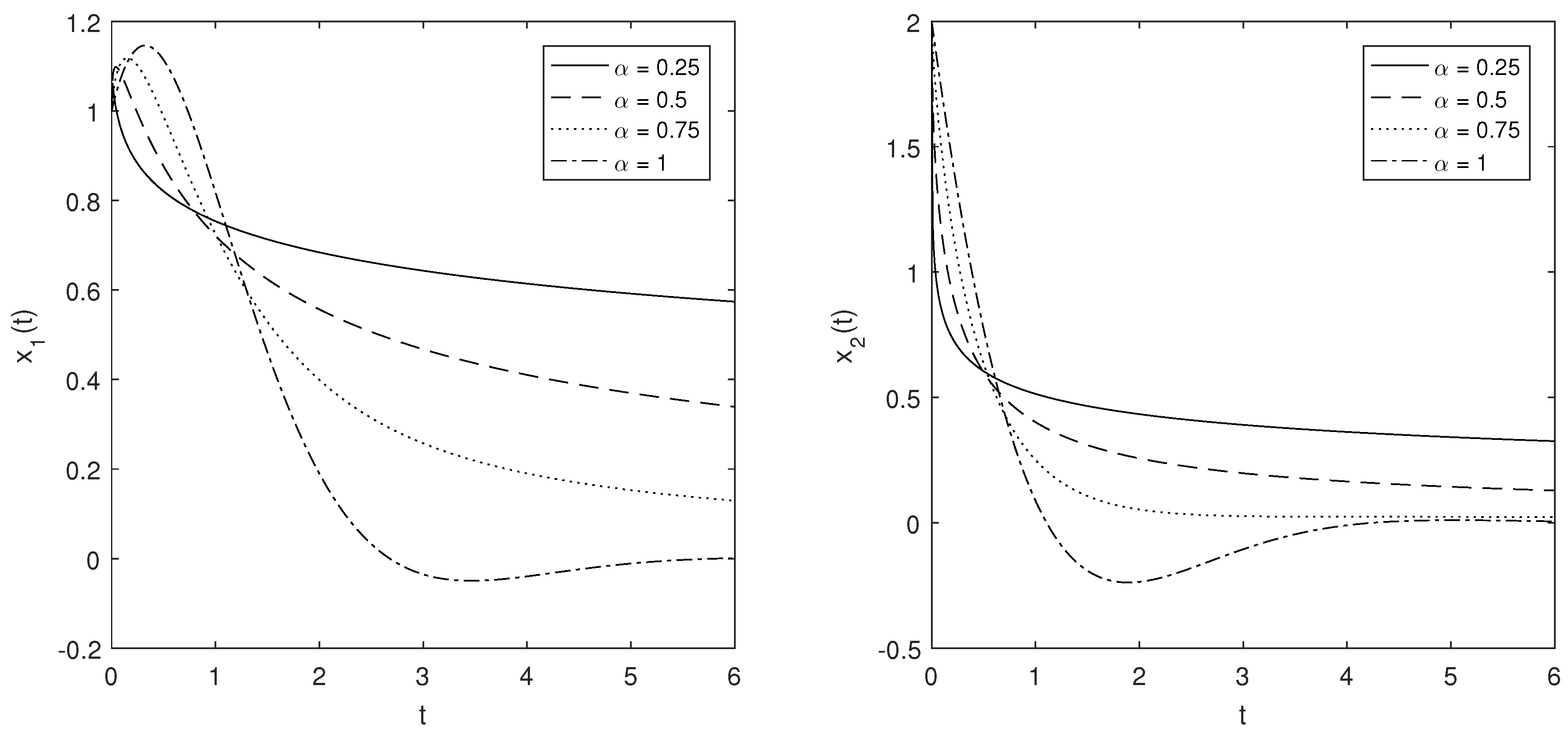
The solution of the initial value problem of Equation (34) parameterized by the order $\alpha$ is

$$\begin{array}{ccc}\hfill \mathbf{x}\left(t\right)& =& E_{\alpha ,1}\left(A{t}^{\alpha }\right)\mathbf{x}\left(0\right)\hfill \\ & =& \frac{1}{2}\left[\begin{array}{c}1+2\mathrm{i}\\ 2-\mathrm{i}\end{array}\right]E_{\alpha ,1}\left({\lambda }_1{t}^{\alpha }\right)+\frac{1}{2}\left[\begin{array}{c}1-2\mathrm{i}\\ 2+\mathrm{i}\end{array}\right]E_{\alpha ,1}\left({\lambda }_2{t}^{\alpha }\right).\hfill \end{array}$$

(37)

If $\alpha =1$, the solution becomes the classical result

$$\begin{array}{ccc}\hfill \mathbf{x}\left(t\right)& =& e^{-t}\left[\begin{array}{c}cost+2sint\\ 2cost-sint\end{array}\right].\hfill \end{array}$$

(38)

In Figure 1, we show the curves of the solutions $x_1\left(t\right)$ and $x_2\left(t\right)$ versus t for different values of $\alpha$.

Example 3.

Consider the solution of the nonhomogeneous initial value problem

$$\begin{array}{c}\hfill D_t^{\alpha }\mathbf{x}\left(t\right)=A\mathbf{x}\left(t\right)+\mathbf{f}\left(t\right),\mathbf{x}\left(0\right)={(0,0)}^T\end{array}$$

(39)

where $\mathbf{f}\left(t\right)={[e^{-t},sint]}^T$ and A is the same second-order matrix as in Example 2.

If $\alpha =1$, the exact solution is

$$\begin{array}{ccc}\hfill \mathbf{x}\left(t\right)& =& exp\left(At\right)\ast \mathbf{f}\left(t\right)\hfill \\ & =& \left(\begin{array}{cc}{e}^{-t}cost& e^{-t}sint\\ -e^{-t}sint& e^{-t}cost\end{array}\right)\ast \left(\begin{array}{c}{e}^{-t}\\ sint\end{array}\right)\hfill \\ & =& \left(\begin{array}{c}\frac{1}{5}(6e^{-t}+1)sint+\frac{2}{5}(e^{-t}-1)cost\\ \frac{1}{5}(-2e^{-t}+3)sint+\frac{1}{5}(6e^{-t}-1)cost-e^{-t}\end{array}\right).\hfill \end{array}$$

(40)

From Equation (20), we have the solution of the nonhomogeneous initial value problem of Equation (39):

$$\begin{array}{ccc}\hfill \mathbf{x}\left(t\right)& =& t^{\alpha }{E}_{\alpha ,\alpha +1}\left(A{t}^{\alpha }\right)\mathbf{f}\left(0\right)+t^{\alpha }{E}_{\alpha ,\alpha +1}\left(A{t}^{\alpha }\right)\ast {\mathbf{f}}^{\prime }\left(t\right)\hfill \end{array}$$

(43)

where $\mathbf{f}\left(0\right)={[1,0]}^T$ and ${\mathbf{f}}^{\prime }\left(t\right)={[-e^{-t},cost]}^T$. Here, we use Equation (20) instead of Equation (13) for the sake of numerical computation of the convolution. From Equation (36), the matrix Mittag–Leffler function has the expression

$$\begin{array}{ccc}\hfill E_{\alpha ,\alpha +1}\left(A{t}^{\alpha }\right)& =& [\frac{1+\mathrm{i}}{2}{E}_{\alpha ,\alpha +1}\left({\lambda }_1{t}^{\alpha }\right)+\frac{1-\mathrm{i}}{2}{E}_{\alpha ,\alpha +1}\left({\lambda }_2{t}^{\alpha }\right)]I\hfill \\ & & +[\frac{\mathrm{i}}{2}{E}_{\alpha ,\alpha +1}\left({\lambda }_1{t}^{\alpha }\right)-\frac{\mathrm{i}}{2}{E}_{\alpha ,\alpha +1}\left({\lambda }_2{t}^{\alpha }\right)]A.\hfill \end{array}$$

In order to numerically calculate the convolution in Equation (41), we denote $t_n=nh,$$n=0,1,\cdots ,N$. Thus, we have $\mathbf{x}\left(t_0\right)=\mathbf{x}\left(0\right)={[0,0]}^T.$ For $1\le n\le N$, we apply the composite trapezoidal rule to the convolution integral in Equation (41):

$$\begin{array}{ccc}\hfill \mathbf{x}\left(t_n\right)& =& t_n^{\alpha }{E}_{\alpha ,\alpha +1}\left(A{t}_n^{\alpha }\right)\mathbf{f}\left(0\right)+{\int }_0^{t_n}{\tau }^{\alpha }{E}_{\alpha ,\alpha +1}\left(A{\tau }^{\alpha }\right){\mathbf{f}}^{\prime }(t_n-\tau )d\tau \hfill \\ & =& t_n^{\alpha }{E}_{\alpha ,\alpha +1}\left(A{t}_n^{\alpha }\right)\mathbf{f}\left(0\right)+\sum _{j=0}^n{\omega }_{n,j}{t}_j^{\alpha }{E}_{\alpha ,\alpha +1}\left(A{t}_j^{\alpha }\right){\mathbf{f}}^{\prime }(t_n-t_j)\hfill \\ & =& t_n^{\alpha }{E}_{\alpha ,\alpha +1}\left(A{t}_n^{\alpha }\right)\mathbf{f}\left(0\right)+\sum _{j=0}^n{\omega }_{n,j}{\left(jh\right)}^{\alpha }{E}_{\alpha ,\alpha +1}\left(A{\left(jh\right)}^{\alpha }\right)\left[\begin{array}{c}-e^{-(n-j)h}\\ cos(n-j)h\end{array}\right]\hfill \end{array}$$

where

$${\omega }_{n,0}={\omega }_{n,n}=h/2,{\omega }_{n,j}=h,j=1,2,\cdots ,n-1.$$

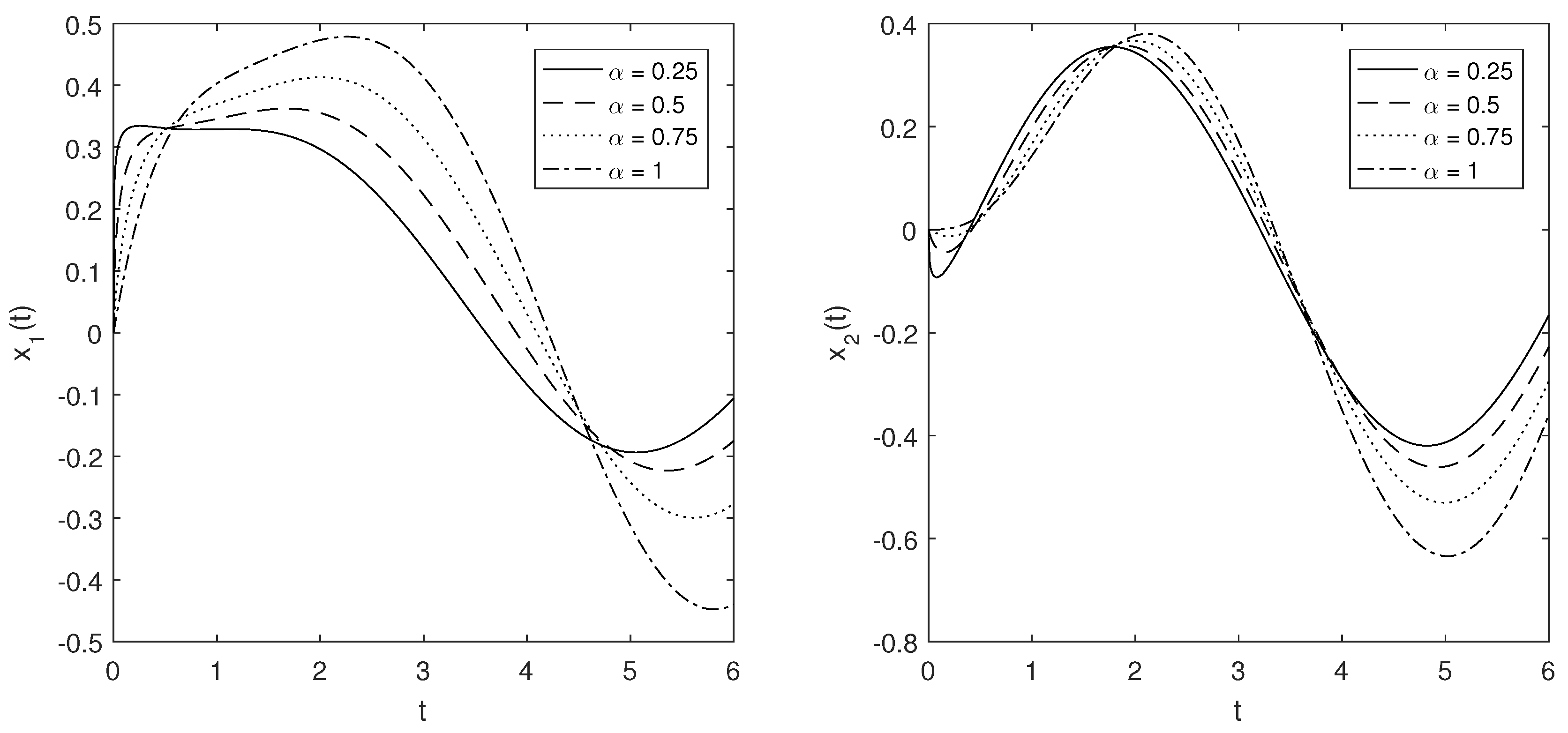
In Figure 2, we plot the curves of the solutions $x_1\left(t\right)$ and $x_2\left(t\right)$ versus t on the interval $0\le t\le 6$ for different values of $\alpha$, where we take $h=0.01$.

Example 4.

Consider the system of fractional differential equations

$$\begin{array}{c}\hfill \left\{\begin{array}{ccc}{D}_t^{2/3}{x}_1\left(t\right)& =& -2x_1-x_2\hfill \\ D_t^{4/15}{x}_2\left(t\right)& =& x_1-x_2\hfill \end{array}\right.\end{array}$$

(44)

subject to the initial condition

$$x_1\left(0\right)=2,x_2\left(0\right)=3.$$

From Section 3, we know that $\beta =\frac{2}{15},$ $p_1=5,p_2=2$. We need to introduce seven variables $y_1,y_2,\cdots ,y_7$, where $x_1=y_1,x_2=y_6,$ and where they satisfy the system

$$\begin{array}{c}\hfill \left\{\begin{array}{c}{D}_t^{\beta }{y}_1\left(t\right)=y_2\hfill \\ D_t^{\beta }{y}_2\left(t\right)=y_3\hfill \\ D_t^{\beta }{y}_3\left(t\right)=y_4\hfill \\ D_t^{\beta }{y}_4\left(t\right)=y_5\hfill \\ D_t^{\beta }{y}_5\left(t\right)=-2y_1-y_6\hfill \\ D_t^{\beta }{y}_6\left(t\right)=y_7\hfill \\ D_t^{\beta }{y}_7\left(t\right)=y_1-y_6\hfill \end{array}\right.\end{array}$$

(45)

subject to the initial value condition

$$\mathbf{y}\left(0\right)={(y_1\left(0\right),y_2\left(0\right),\cdots ,y_7\left(0\right))}^T={(2,0,0,0,0,3,0)}^T.$$

In the system of commensurate orders of Equation (43), the coefficient matrix is

$$A=\left[\begin{array}{ccccccc}0& 1& 0& 0& 0& 0& 0\\ 0& 0& 1& 0& 0& 0& 0\\ 0& 0& 0& 1& 0& 0& 0\\ 0& 0& 0& 0& 1& 0& 0\\ -2& 0& 0& 0& 0& -1& 0\\ 0& 0& 0& 0& 0& 0& 1\\ 1& 0& 0& 0& 0& -1& 0\end{array}\right],$$

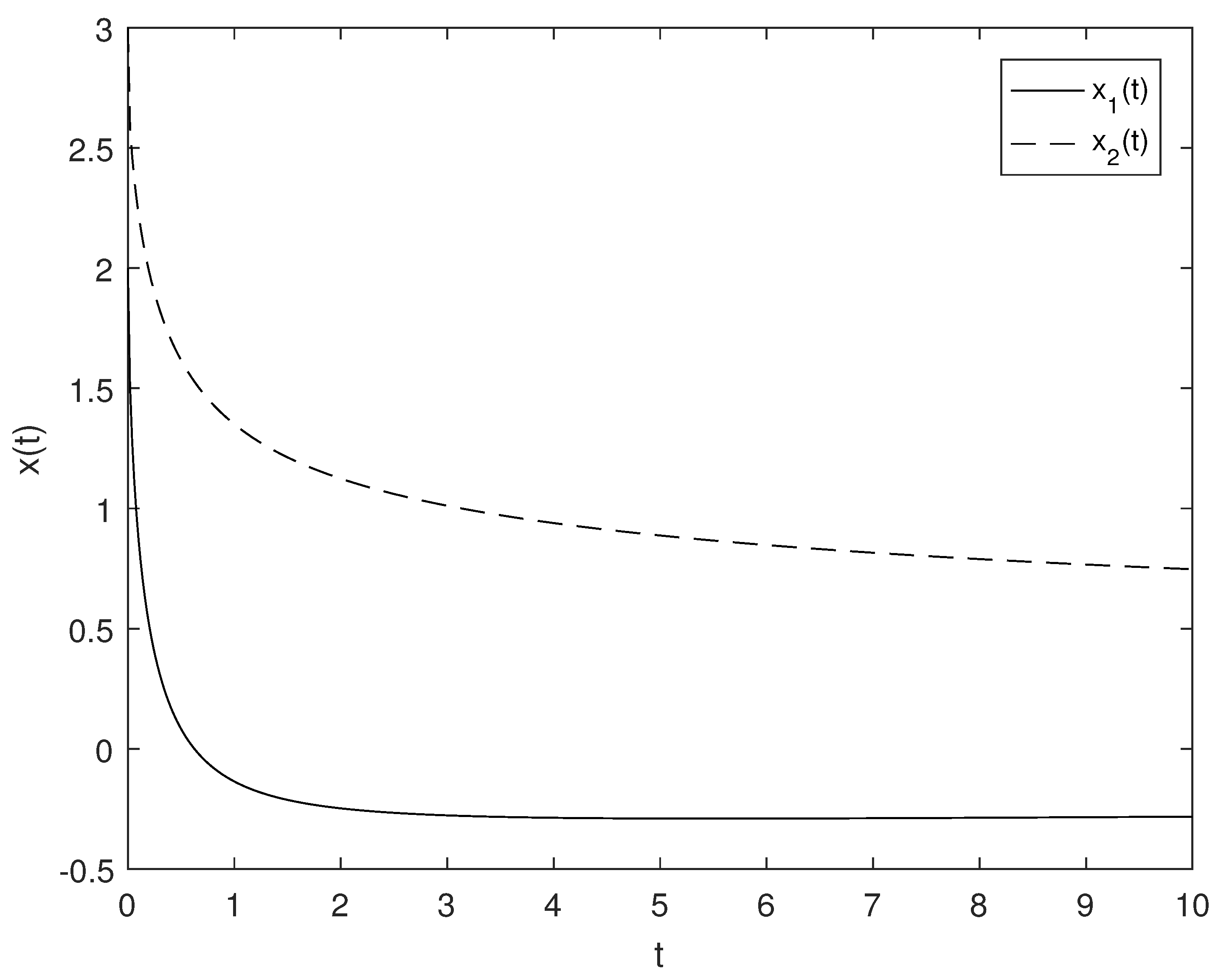
which has seven different eigenvalues $-1.1926,-0.4639\pm 1.0830\mathrm{i},0.0778\pm 1.1275\mathrm{i},0.9824\pm 0.6734\mathrm{i}.$ The solution $E_{\beta ,1}\left(A{t}^{\beta }\right)\mathbf{y}\left(0\right)$ may be calculated using the methods in Section 4. We plot the solutions $x_1\left(t\right)$ and $x_2\left(t\right)$ of the original system in Figure 3.

A major disadvantage of the Jordan canonical form is that the involved similarity transformation can be ill-conditioned [46].

6. Conclusions

The solutions of system of linear fractional differential equations were considered. For the case of commensurate orders, we derived the solution in terms of matrix Mittag–Leffler functions using the Picard iterative process. For the case of incommensurate orders, through introducing new unknown functions, we constructed a system of commensurate orders. We then investigated how a matrix Mittag–Leffler function can be calculated. We discussed two methods, i.e., the Jordan canonical matrix and the minimal polynomial or eigenpolynomial, to express the matrix Mittag–Leffler function $E_{\alpha ,\rho }\left(A{t}^{\alpha }\right)$ into a matrix polynomial, where the coefficients were given in terms of scalar Mittag–Leffler functions $E_{\alpha ,\rho }\left(\lambda t^{\alpha }\right)$, which may be calculated using the MATLAB code [44,45]. Finally, we solved numerical examples by using the proposed methods. Solutions were plotted using MATLAB.

References

- Oldham, K.B.; Spanier, J. The Fractional Calculus; Academic: New York, NY, USA, 1974. [Google Scholar]
- Ross, B. (Ed.) Fractional Calculus and Its Applications (Lecture Notes in Mathematics 457); Springer: Berlin, UK, 1975. [Google Scholar]
- Miller, K.S.; Ross, B. An Introduction to the Fractional Calculus and Fractional Differential Equations; Wiley: New York, NY, USA, 1993. [Google Scholar]
- Carpinteri, A.; Mainardi, F. (Eds.) Fractals and Fractional Calculus in Continuum Mechanics; Springer: Wien, Austria; New York, NY, USA, 1997. [Google Scholar]
- Podlubny, I. Fractional Differential Equations; Academic: San Diego, CA, USA, 1999. [Google Scholar]
- Kilbas, A.A.; Srivastava, H.M.; Trujillo, J.J. Theory and Applications of Fractional Differential Equations; Elsevier: Amsterdam, The Netherlands, 2006. [Google Scholar]
- Diethelm, K. The Analysis of Fractional Differential Equations; Springer: Berlin, UK, 2010. [Google Scholar]
- Mainardi, F. Fractional Calculus and Waves in Linear Viscoelasticity; Imperial College: London, UK, 2010. [Google Scholar]
- Mainardi, F.; Spada, G. Creep, relaxation and viscosity properties for basic fractional models in rheology. Eur. Phys. J. Spec. Top. 2011, 193, 133–160. [Google Scholar] [CrossRef] [Green Version]
- Li, M. Three classes of fractional oscillators. Symmetry 2018, 10, 40. [Google Scholar] [CrossRef]
- Mainardi, F. Fractional relaxation-oscillation and fractional diffusion-wave phenomena. Chaos Solitons Fractals 1996, 7, 1461–1477. [Google Scholar] [CrossRef]
- Metzler, R.; Klafter, J. The random walk’s guide to anomalous diffusion: A fractional dynamics approach. Phys. Rep. 2000, 339, 1–77. [Google Scholar] [CrossRef]
- Duan, J.S. Time- and space-fractional partial differential equations. J. Math. Phys. 2005, 46, 13504–13511. [Google Scholar] [CrossRef]
- Wu, G.C.; Baleanu, D.; Zeng, S.D.; Deng, Z.G. Discrete fractional diffusion equation. Nonlinear Dyn. 2015, 80, 281–286. [Google Scholar] [CrossRef]
- Monje, C.A.; Chen, Y.Q.; Vinagre, B.M.; Xue, D.; Feliu, V. Fractional-Order Systems and Controls, Fundamentals and Applications; Springer: London, UK, 2010. [Google Scholar]
- Wu, G.C.; Baleanu, D.; Xie, H.P.; Chen, F.L. Chaos synchronization of fractional chaotic maps based on the stability condition. Physica A 2016, 460, 374–383. [Google Scholar] [CrossRef]
- Cao, W.; Xu, Y.; Zheng, Z. Existence results for a class of generalized fractional boundary value problems. Adv. Differ. Equ. 2017, 2017, 348. [Google Scholar] [CrossRef]
- Băleanu, D.; Diethelm, K.; Scalas, E.; Trujillo, J.J. Fractional Calculus Models and Numerical Methods; Series on Complexity, Nonlinearity and Chaos; World Scientific: Boston, UK, 2012. [Google Scholar]
- Li, M.; Lim, S.C.; Chen, S. Exact solution of impulse response to a class of fractional oscillators and its stability. Math. Probl. Eng. 2011, 2011, 657839. [Google Scholar] [CrossRef]
- Li, C.; Zeng, F. Numerical Methods for Fractional Calculus; CRC Press: Boca Raton, FL, USA, 2015. [Google Scholar]
- Jafari, H.; Khalique, C.M.; Ramezani, M.; Tajadodi, H. Numerical solution of fractional differential equations by using fractional B-spline. Cent. Eur. J. Phys. 2013, 11, 1372–1376. [Google Scholar] [CrossRef] [Green Version]
- Mainardi, F.; Gorenflo, R. On Mittag–Leffler-type functions in fractional evolution processes. J. Comput. Appl. Math. 2000, 118, 283–299. [Google Scholar] [CrossRef]
- Garra, R.; Gorenflo, R.; Polito, F.; Tomovski, Ž. Hilfer-Prabhakar derivatives and some applications. Appl. Math. Comput. 2014, 242, 576–589. [Google Scholar] [CrossRef]
- Garrappa, R.; Mainardi, F.; Guido, M. Models of dielectric relaxation based on completely monotone functions. Frac. Calc. Appl. Anal. 2016, 19, 1105–1160. [Google Scholar] [CrossRef]
- Fernandez, A.; Baleanu, D.; Srivastava, H.M. Series representations for fractional-calculus operators involving generalised Mittag–Leffler functions. Commun. Nonlinear Sci. Numer. Simul. 2019, 67, 517–527. [Google Scholar] [CrossRef]
- Srivastava, H.M. Some families of Mittag–Leffler type functions and associated operators of fractional calculus. TWMS J. Pure Appl. Math. 2016, 7, 123–145. [Google Scholar]
- Tomovski, Z.; Hilfer, R.; Srivastava, H.M. Fractional and operational calculus with generalized fractional derivative operators and Mittag–Leffler type functions. Integral Transform. Spec. Funct. 2010, 21, 797–814. [Google Scholar] [CrossRef]
- Atanackovic, T.M.; Stankovic, B. On a system of differential equations with fractional derivatives arising in rod theory. J. Phys. A 2004, 37, 1241–1250. [Google Scholar] [CrossRef]
- Garrappa, R. Exponential integrators for time-fractional partial differential equations. Eur. Phys. J. Spec. Top. 2013, 222, 1915–1927. [Google Scholar] [CrossRef]
- Daftardar-Gejji, V.; Babakhani, A. Analysis of a system of fractional differential equations. J. Math. Anal. Appl. 2004, 293, 511–522. [Google Scholar] [CrossRef]
- Deng, W.; Li, C.; Lü, J. Stability analysis of linear fractional differential system with multiple time delays. Nonlinear Dyn. 2007, 48, 409–416. [Google Scholar] [CrossRef]
- Charef, A.; Boucherma, D. Analytical solution of the linear fractional system of commensurate order. Comput. Math. Appl. 2011, 62, 4415–4428. [Google Scholar] [CrossRef]
- Duan, J.S.; Fu, S.Z.; Wang, Z. Solution of linear system of fractional differential equations. Pac. J. Appl. Math. 2013, 5, 93–106. [Google Scholar]
- Daftardar-Gejji, V.; Jafari, H. Adomian decomposition: A tool for solving a system of fractional differential equations. J. Math. Anal. Appl. 2005, 301, 508–518. [Google Scholar] [CrossRef]
- Duan, J. A generalization of the Mittag–Leffler function and solution of system of fractional differential equations. Adv. Differ. Equ. 2018, 2018, 239. [Google Scholar] [CrossRef]
- Garrappa, R.; Moret, I.; Popolizio, M. On the time-fractional Schrödinger equation: Theoretical analysis and numerical solution by matrix Mittag–Leffler functions. Comput. Math. Appl. 2017, 74, 977–992. [Google Scholar] [CrossRef]
- Moret, I.; Novati, P. On the convergence of Krylov subspace methods for matrix Mittag–Leffler functions. SIAM J. Numer. Anal. 2011, 49, 2144–2164. [Google Scholar] [CrossRef]
- Matychyn, I.; Onyshchenko, V. Matrix Mittag–Leffler function in fractional systems and its computation. Bull. Pol. Acad. Sci. Tech. Sci. 2018, 66, 495–500. [Google Scholar]
- Garrappa, R.; Popolizio, M. Computing the matrix Mittag–Leffler function with applications to fractional calculus. J. Sci. Comput. 2018, 77, 129–153. [Google Scholar] [CrossRef]
- Garrappa, R. Numerical evaluation of two and three parameter Mittag–Leffler functions. SIAM J. Numer. Anal. 2015, 53, 1350–1369. [Google Scholar] [CrossRef]
- Garrappa, R.; Popolizio, M. Generalized exponential time differencing methods for fractional order problems. Comput. Math. Appl. 2011, 62, 876–890. [Google Scholar] [CrossRef]
- Popolizio, M. Numerical solution of multiterm fractional differential equations using the matrix Mittag–Leffler functions. Mathematics 2018, 6, 7. [Google Scholar] [CrossRef]
- Horn, R.A.; Johnson, C.R. Matrix Analysis, 2nd ed.; Cambridge University: New York, NY, USA, 2013. [Google Scholar]
- Podlubny, I. Mittag–Leffler function; Calculates the Mittag–Leffler function with desired accuracy. MATLAB Central/File Exchange (Updated September 2012), version 1.2.0.0; Available online: https://www.mathworks.com/matlabcentral/fileexchange/8738-mittag-leffler-function (accessed on 14 October 2018).
- Garrappa, R. The Mittag–Leffler function; Evaluation of the Mittag–Leffler function with 1, 2 or 3 parameters. MATLAB Central/File Exchange (Updated December 2015), version 1.3.0.0; Available online: https://au.mathworks.com/matlabcentral/fileexchange/48154-the-mittag-leffler-function (accessed on 14 October 2018).
- Higham, N.J. Functions of Matrices: Theory and Computation; SIAM: Philadephia, PA, USA, 2008. [Google Scholar]
Figure 1.
Curves of solutions (left) and (right) of Example 2 versus t for (solid line), (dash line), (dot line), and (dot-dash line).
Figure 2.
Curves of solutions (left) and (right) of Example 3 versus t for (solid line), (dash line), (dot line), and (dot-dash line).
Figure 3.
Curves of solutions (solid line) and (dash line) of Example 4 versus t.
© 2018 by the authors. Licensee MDPI, Basel, Switzerland. This article is an open access article distributed under the terms and conditions of the Creative Commons Attribution (CC BY) license (http://creativecommons.org/licenses/by/4.0/).
Share and Cite
MDPI and ACS Style
Duan, J.; Chen, L. Solution of Fractional Differential Equation Systems and Computation of Matrix Mittag–Leffler Functions. Symmetry 2018, 10, 503. https://doi.org/10.3390/sym10100503
AMA Style
Duan J, Chen L. Solution of Fractional Differential Equation Systems and Computation of Matrix Mittag–Leffler Functions. Symmetry. 2018; 10(10):503. https://doi.org/10.3390/sym10100503
Chicago/Turabian StyleDuan, Junsheng, and Lian Chen. 2018. "Solution of Fractional Differential Equation Systems and Computation of Matrix Mittag–Leffler Functions" Symmetry 10, no. 10: 503. https://doi.org/10.3390/sym10100503
Note that from the first issue of 2016, this journal uses article numbers instead of page numbers. See further details here.