Article

A Semi-Supervised Model for Top-N Recommendation

Science and Technology on Parallel and Distributed Laboratory, College of Computer, National University of Defense Technology, Changsha 410073, China
*
Author to whom correspondence should be addressed.
Symmetry 2018, 10(10), 492; https://doi.org/10.3390/sym10100492
Submission received: 11 September 2018 / Revised: 4 October 2018 / Accepted: 8 October 2018 / Published: 12 October 2018

Abstract

:
Top-N recommendation is an important recommendation technique that delivers a ranked top-N item list to each user. Data sparsity is a great challenge for top-N recommendation. In order to tackle this problem, in this paper, we propose a semi-supervised model called Semi-BPR (Semi-Supervised Bayesian Personalized Ranking). Our approach is based on the assumption that, for a given model, users always prefer items ranked higher in the generated recommendation list. Therefore, we select a certain number of items ranked higher in the recommendation list to construct an intermediate set and optimize the metric Area Under the Curve (AUC). In addition, we treat the intermediate set as a teaching set and design a semi-supervised self-training model. We conduct a series of experiments on three popular datasets to compare the proposed approach with several state-of-the-art baselines. The experimental results demonstrate that our approach significantly outperforms the other methods for all evaluation metrics, especially for sparse datasets.

1. Introduction

Along with the rapid expansion of the Internet, recommender systems are becoming very popular tools to help users discover information that interests them and to alleviate information overload problems. In recent years, recommender systems have received more and more attention and have been widely applied in many areas, such as e-commerce, social network and online video sites.
Generally speaking, there are two main categories of recommendation tasks: rating prediction tasks and top-N recommendation tasks. The goal of rating prediction tasks is to predict users’ ratings for unrated items. Early research mostly focused on this kind of task, for example a Netflix prize competition [1]. Models for rating prediction tasks mainly rely on users’ explicit feedback (i.e., numerical ratings) to make predictions. However, users’ explicit feedback is usually very scarce and hard to acquire. On the contrary, implicit feedback (such as purchase history, browsing history, etc.) is much easier to collect, and the amount is abundant. Top-N recommendation models only need implicit feedback to make recommendations. The objective of top-N recommendation is to generate a ranked item list for each user. The application scenario is very common in real life, for example product recommendations on Amazon [2], video recommendations on YouTube and friend recommendations on Facebook. Therefore, many recent studies have switched from using a rating prediction task to a top-N recommendation task. In this paper, we mainly consider the top-N recommendation issue.
For top-N recommendation with implicit feedback, the existing approaches can be further divided into two categories: pointwise methods and pairwise methods. Pointwise methods learn the model parameters by minimizing a pointwise loss function to approximate the absolute rating values. In contrast, based on the assumption that users prefer rated items to unrated items, pairwise methods directly optimize the ranking-oriented metrics, such as the AUC (Area Under the Curve), the MAP (Mean Average Precision), the MRR (Mean Reciprocal Rank), etc. Empirically, the pairwise methods always achieve much better performance than the pointwise methods.
An important challenge is that top-N recommendation with implicit feedback faces a lack of negative samples. In fact, the missing ratings are a mixture of unobserved positive feedback and negative feedback and are difficult to distinguish. Most existing pairwise methods directly treat the missing ratings the same as negative feedback and assume that users prefer rated over unrated items. However, this neglects users’ relative preference relations among the unrated items, which may cause performance degradation.
In order to exploit users’ fine-grained preference over the unobserved feedback, we assumed that for a given recommendation model, users always prefer items ranked higher in the generated recommendation list. To test this assumption, we used the Bayesian Personalized Ranking (BPR) model to generate a recommendation list for each user in the Movielens 1M dataset. Figure 1 shows the average hit rate at different positions of the list. We observed that items ranked higher in the recommendation list had a higher hit rate. That is to say, users always preferred items ranked higher than items ranked lower in the recommendation list.
For each user, we first randomly selected a certain number of unrated items to construct an intermediate set, and the remaining unrated items were treated as negative feedback. We assumed that users preferred items with positive feedback over items in the intermediate set and that they preferred items in the intermediate set over items with negative feedback. This assumption not only takes account of users’ preferences over observed and unobserved items, but also users’ preferences among the unobserved items. Based on this assumption, we directly optimized the AUC metric to place the item with positive feedback at the top, items belonging to the intermediate set in the middle and items with negative feedback at the bottom of the recommendation list. Then, we selected some items ranked higher in the newly generated recommendation list to update the intermediate set. It is possible to repeat the above cycle to iteratively improve the performance in a self-training paradigm.
The contributions of our work can be summarized as follows:
  • We made an assumption about users’ relative preferences among unrated items and put forward an approach to build an intermediate set and optimize the AUC metric.
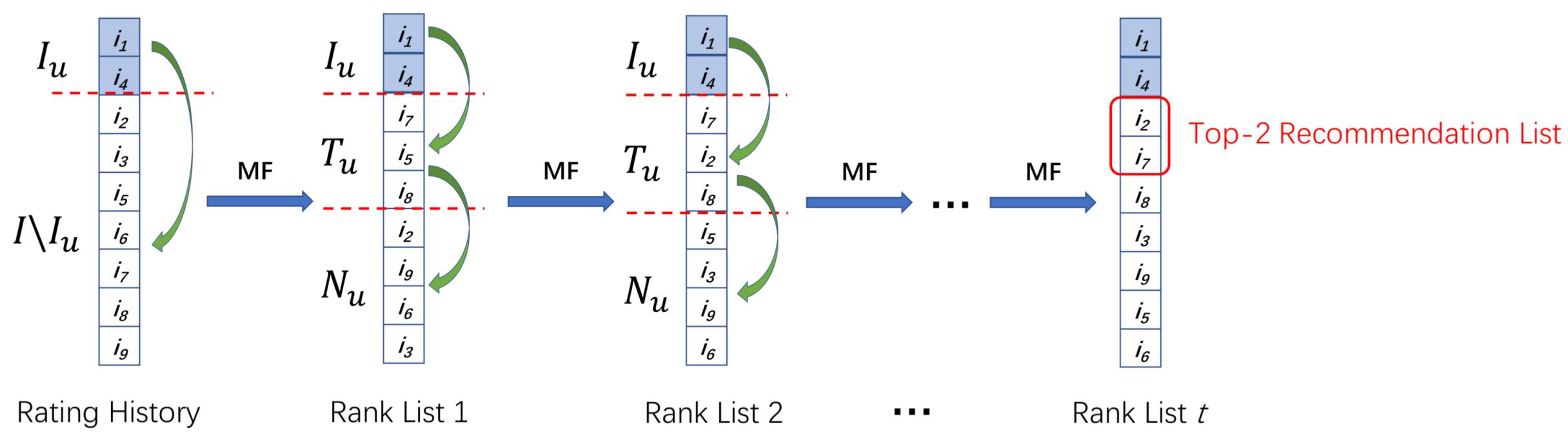
  • We used the intermediate set as a teaching set and designed a semi-supervised self-training model.
  • We conducted extensive experiments on three popular datasets, and the experimental results demonstrated the effectiveness of our approach.
The remainder of this paper is constructed as follows: We discuss the related work in Section 2. Section 3 describes our approach in detail. In Section 4, we analyze the experimental results. Finally, Section 5 concludes the paper.

2. Related Work

In this paper, we focus primarily on top-N recommendation with implicit feedback, and the key innovation of our approach is a semi-supervised self-training paradigm. Hence, we discuss the related work about the top-N recommendation and semi-supervised recommendation methods separately.

2.1. Top-N Recommendation

In top-N recommendation tasks, the objective is to recommend a list of products to each user that is most favorable. There are two major categories of top-N recommendation methods: pointwise methods and pairwise methods.
Pointwise methods learn the model parameters by minimizing a pointwise loss function to fit users’ absolute rating values. Pan et al. [3] formulated the One-Class Collaborative Filtering (OCCF) problem and presented two methods to solve this problem: one is based on negative example weighting and the other on negative example exampling. Hu et al. [4] treated users’ rating data as indications of positive and negative preferences, which are associated with different confidence values. They also put forward a scalable optimization procedure tailored to implicit feedback recommenders. Ning et al. [5] presented the Sparse Linear Method (SLIM) for top-N recommendation, which learns a sparse aggregation coefficient matrix for items by solving a regularized optimization problem. To improve the effectiveness of top-N recommendation, Kabbur et al. [6] presented Factored Item Similarity Models (FISM) for top-N recommendation. In their model, the item-item similarity matrix is decomposed into the product of two low rank latent factor matrices.
Based on the assumption that users prefer the rated items to the unrated items, pairwise methods attempt to directly optimize ranking-oriented metrics. The work in [7] is a seminal work for pairwise recommendation. A general OPTimization criterion for Bayesian Personalized Ranking (BPR-OPT) is proposed in this paper. By introducing richer interactions among users, Pan et al. [8] put forward the Group Bayesian Personalized Ranking (GBPR) model. Shi et al. [9] presented the Collaborative Less is More Filtering (CLiMF) model by directly maximizing the metric MRR. The work in [10] proposed the Tensor Factorization for MAP Maximization (TFMAP) model as a context-aware top-N recommendation model, by maximizing the MAP metric. Empirically, these pairwise methods can achieve much better performances than pointwise methods. However, these methods treat all of the unobserved feedback as negative feedback, which neglects users’ relative preferences among the unobserved items. In addition, this separation causes an extreme imbalance between positive and negative samples.
Recently, a few studies have tried to solve this problem. Based on the assumption that users tend to prefer items that their friends select, Zhao et al. [11] developed a model called SBPR (Social Bayesian Personalized Ranking). Song et al. [12] put forward a Generalized AUC (GAUC) metric to quantify the ranking performance in a signed social network. Based on the idea that users tend to prefer items selected by their neighbors, Liu et al. [13] proposed a top-N recommendation algorithm called Collaborative Pairwise Learning to Rank (CPLR). Lu Yu et al. [14] tried to incorporate multiple types of user-item relationships into a unified pairwise ranking model to optimize approximately the MAP and MRR ranking metrics. Although these few methods exploit the user’s preference among the unobserved items, they are all based on heuristic rules, and their performance is not satisfactory. Compared with these methods, our approach is more flexible and does not require any auxiliary information.

2.2. Semi-Supervised Recommendation

Semi-supervised learning [15] has been investigated thoroughly in the traditional data mining fields, such as classification and regression. However, little research has been conducted in the field of recommender systems.
Zhang et al. [16] proposed a semi-supervised ensemble recommendation model. By employing the co-training strategy, this model allows two weak prediction models to learn from each other. To further improve its performance, The work in [17] designed a tri-training framework to incorporate more recommender models. The work in [18] presented a background-based semi-supervised tri-training model. These semi-supervised recommendation methods are all designed for item rating prediction tasks, but are inappropriate for top-N recommendation tasks.
The work in [19] proposed a semi-supervised multi-view ranking algorithm for document ranking, which takes advantage of the global consistency between view-specific ranking functions on unlabeled samples. This algorithm can enhance the document ranking performance, but it relies on multiple view information, which is usually not available in the recommender system field. The work in [20] presented a semi-supervised model for bipartite ranking based on the self-training paradigm. Although this model and our model are both based on the self-training paradigm, they are actually quite different. First, the model of [20] is designed for bipartite ranking tasks, where both positive and negative samples are available. However, for top-N recommendation tasks with implicit feedback, there are only positive samples. Second, the ranking cost functions are quite different. In our model, we directly optimize the AUC metric, which can allow a higher recommendation performance to be obtained.

3. Our Approach

In this section, we first formulate the top-N recommendation with implicit feedback problem and then introduce the motivation of our approach. After that, we describe the design of our approach in detail. Finally, we present the model learning method and analyze its computational complexity.

3.1. Problem Definition
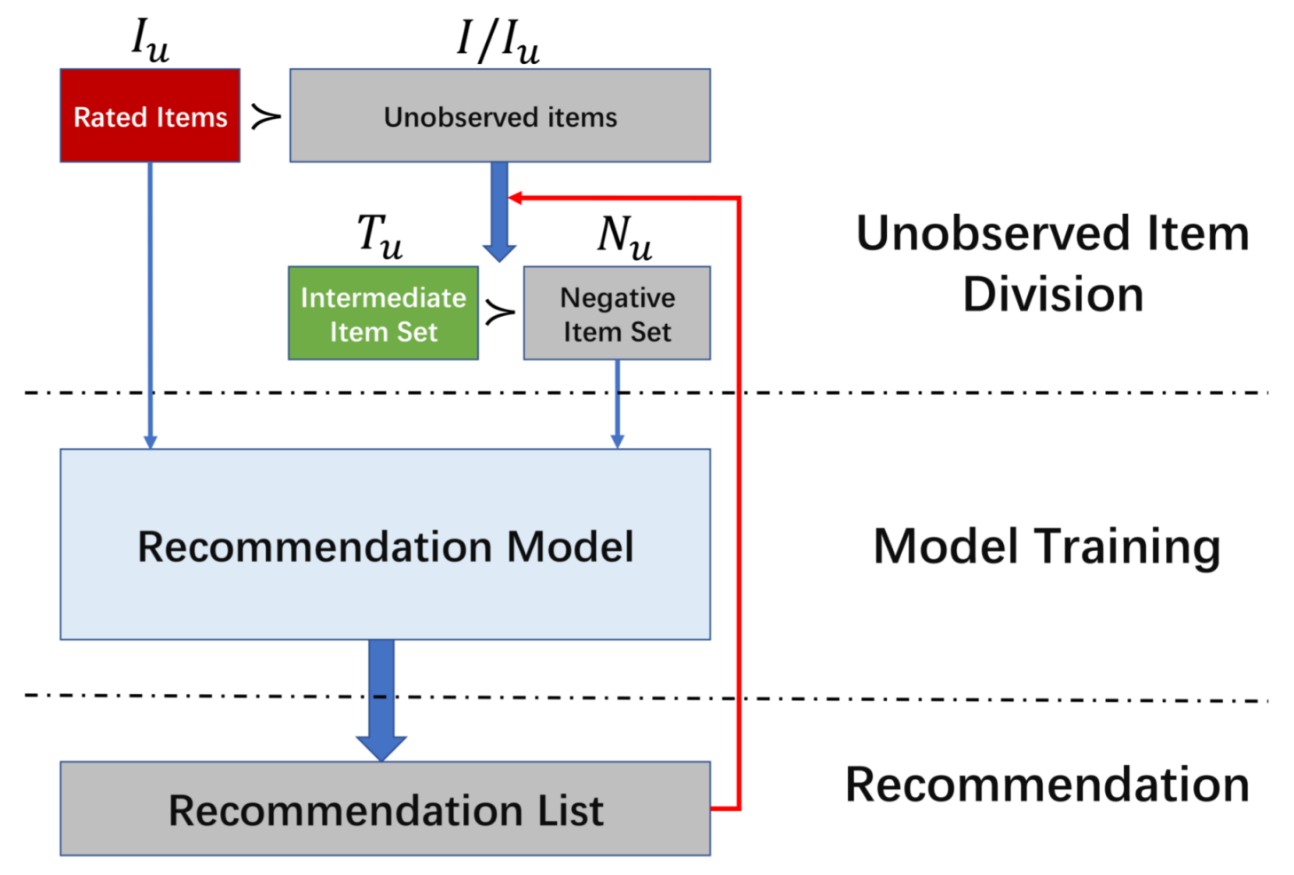
Some symbols that are frequently used in the rest of the paper are summarized in Table 1. The top-N recommendation problem can be described as follows: given the user-item implicit feedback matrix R m × n from m users and n items, the goal is to learn a scoring function, f u : I / I u R , for each user ( u U ), and to generate a ranking list that is sorted by the scoring values in descending order.

3.2. Overview

If a user’s feedback for an item is observed, we can infer that he/she is interested in the item to a large extent. Thus, we also assume that each user prefers items with positive feedback to items with unobserved feedback.
( u , i ) ( u , j ) , i I u , j I / I u
where ( u , i ) and ( u , j ) refer to the user’s preferences for item i and item j, respectively. The symbol ≻ represents the user’s relative preference.
In many cases, the user-item rating matrix is very sparse. If a user has not rated an item, he may not like this item. Therefore, treating all the unrated items as negative samples has a certain degree of rationality. However, this separation neglects users’ relative preferences over unrated items.
In the recommendation list of user u, if item j is ranked higher than item k, we think the probability that u likes item j is greater than that of item k. If their ranking difference is large enough, we can almost infer user u prefers item j to item k. This can be represented as the following equation:
( u , j ) ( u , k ) , j , k I / I u , r a n k u ( j ) < r a n k u ( k )
where r a n k u ( j ) and r a n k u ( k ) refer to the ranking positions of item j and item k in the recommendation list of user u, respectively.
According to the generated recommendation list, we can divide the unobserved items of user u into two subsets: intermediate item set T u and negative item set N u . Specifically, we select the top 0 < r < 1 proportion of the items in the recommendation list to construct an intermediate item set, and the remaining unobserved items construct a negative item set. Then, it is assumed that each user prefers items in the intermediate item set to items in the negative item set.
( u , j ) ( u , k ) , j T u , k N u
where T u N u = , T u N u = I / I u .
According to Equation (1) and Equation (3), we can get the following equation:
( u , i ) ( u , j ) , ( u , i ) ( u , k ) , ( u , j ) ( u , k ) , i I u , j T u , k N u .
Based on the transitive property of the user’s relative preference (≻), Equation (4) can be simplified to:
( u , i ) ( u , j ) , ( u , j ) ( u , k ) , i I u , j T u , k N u .
According to the above formula, our model assumption can be summarized as follows: each user (u) prefers his/her rated items ( I u ) over items in the intermediate set ( T u ) and prefers items in the intermediated set ( T u ) to items in the negative item set ( N u ).
From the model’s assumptions, we can see that the division of the intermediated item set (T) and the negative item set (N) is critical in our model. However, for a given model, the recommendation list it generates may not be accurate. Division, according to this inaccurate recommendation list, may introduce errors. In order to solve this problem, a self-training paradigm was adopted to improve the model iteratively. An overview of our approach is shown in Figure 2.
In order to illustrate our idea clearly, we performed a case study on a particular user ( u ) , as shown in Figure 3. Suppose there are n = 9 items, namely i 1 i 9 , and user u has the rated items i 1 and i 4 . The goal is to recommend t o p N = 2 unrated items that are most favorable to user u. Based on the assumption that user u prefers the rated items ( I u = { i 1 , i 4 } ) to the unrated items ( I / I u = { i 2 , i 3 , i 5 , i 6 , i 7 , i 8 , i 9 } ), a ranked item list (Rank List 1) can be formed by the Matrix Factorization (MF) model. According to Rank List 1, the unrated items of u can be divided into two subsets: the intermediate item set, T u = { i 7 , i 5 , i 8 } , and the negative item set, N u = { i 2 , i 9 , i 6 , i 3 } . Based on our assumption in Equation (5), user u prefers the items in I u to the items in T u and prefers the items in T u to the items in N u . By optimizing the AUC metric to put items in I u = { i 1 , i 4 } at the top, items in T u = { i 7 , i 5 , i 8 } in the middle and items in N u = { i 2 , i 9 , i 6 , i 3 } at the bottom of the ranked item list, we can get a new ranked item list: Rank List 2. Then, according to Rank List 2, the unrated items ( I / I u ) are divided into T u and N u . The above process is repeated until the ranked item list does not change. Finally, the top two unrated items in the ranked items list are selected to recommend to user u.

3.3. Objective Function

For a given user u, the likelihood of the user’s pairwise preference can be presented by the following equation:
( i , j , k ) I × I × I P ( f u ( i ) > f u ( j ) > f u ( k ) ) δ ( ( u , i ) ( u , j ) ( u , k ) ) × [ 1 - P ( f u ( i ) > f u ( j ) > f u ( k ) ) ] 1 - δ ( ( u , i ) ( u , j ) ( u , k ) ) = i I u j T u k N u P ( f u ( i ) > f u ( j ) ) P ( f u ( j ) > f u ( k ) ) × [ 1 - P ( f u ( i ) < f u ( j ) ) ] [ 1 - P ( f u ( j ) < f u ( k ) ) ]
where δ ( x ) is the indicator function of the Boolean variable x.
δ ( x ) = 1 , i f x i s t r u e 0 , e l s e
It is assumed that the preferences of different users are independent. Therefore, the overall likelihood of all users can be presented as follows:
u U i I u j T u k N u P ( f u ( i ) > f u ( j ) ) P ( f u ( j ) > f u ( k ) ) × [ 1 - P ( f u ( i ) < f u ( j ) ) ] [ 1 - P ( f u ( j ) < f u ( k ) ) ] .
Like the BPR model [7], the function σ ( f u ( i ) - f u ( j ) ) = 1 1 + e - ( f u ( i ) - f u ( j ) ) is used to approximate probability P ( f u ( i ) > f u ( j ) ) . Based on the properties of the sigmoid function ( σ ( · ) ), we have:
P ( f u ( i ) > f u ( j ) ) P ( f u ( j ) > f u ( k ) ) [ 1 - P ( f u ( i ) < f u ( j ) ) ] [ 1 - P ( f u ( j ) < f u ( k ) ) ] = σ ( f u ( i ) - f u ( j ) ) σ ( f u ( j ) - f u ( k ) ) [ 1 - σ ( f u ( j ) - f u ( i ) ) ] [ 1 - σ ( f u ( k ) - f u ( j ) ) ] = [ σ ( f u ( i ) - f u ( j ) ) ] 2 · [ σ ( f u ( j ) - f u ( k ) ) ] 2 .
Based on Equations (8) and (9), the log of the overall likelihood can be obtained, as shown below:
u U i I u j T u k N u 2 · [ l n σ ( f u ( i ) - f u ( j ) ) + l n σ ( f u ( j ) - f u ( k ) ) ] .
Maximizing the log-likelihood is equivalent to maximizing the following object function:
1 2 u U i I u j T u k N u [ l n σ ( f u ( i ) - f u ( j ) ) + l n σ ( f u ( j ) - f u ( k ) ) ] - λ 2 Θ F 2
where Θ are the model parameters and - λ 2 Θ F 2 is the regularization term to avoid overfitting.
AUC is an important metric for measuring the recommendation performance. However, the standard AUC metric only considers binary cases and is not suitable for our situation where there are three kinds of items. Similar to [11] and [12], we defined the AUC of user u as follows:
A U C ( u ) = 1 | I u | · | T u | · | N u | i I u j T u k N u δ ( f u ( i ) - f u ( j ) > 0 ) + δ ( f u ( j ) - f u ( k ) > 0 ) 2 .
By comparing Equations (11) and (12), the log-likelihood and the AUC metric are shown to be very similar. If the normalization term 1 | I u | · | T u | · | N u | of Equation (12) is neglected, the only difference is the loss functions l n σ ( x ) and δ ( x > 0 ) . Because the function δ ( x > 0 ) is non-differential and difficult to optimize, the log-likelihood can be regarded as an approximation of the AUC metric, by replacing δ ( x > 0 ) with the differentiable function l n σ ( x ) .
However, there is a problem with the objective function. According to Equation (11), each sample pair has the same weight and contribution to the model in the training phase. In fact, users’ relative preferences between different sample pairs are quite different. Therefore, we introduced a coefficient to control the weights of each sample pair. The ultimate objective function of our model is defined as the following:
L = 1 2 u U i I u j T u k N u [ a · l n σ ( f u ( i ) - f u ( j ) ) + ( 1 - a ) · l n σ ( f u ( j ) - f u ( k ) ) ] - λ 2 Θ F 2
where a [ 0 , 1 ] is the weight of a user’s relative preference between item i I u and item j T u and 1 - a is the weight of a user’s relative preference between item j T u and item k N u . The larger the probability of item j T u being a positive sample, the smaller coefficient a is.
From Figure 1, it can be observed that items ranked higher in the recommendation list have a higher hit rate, which means items ranked higher are more likely to be a positive sample. Thus, coefficient a can be defined as follows:
a = γ + β ( x u j ) α
where x u j = r a n k u ( j ) | T u | is the relative ranking position of item j in the intermediate item set T u . α , β , γ are adjustable parameters that satisfy α > 0 , 0 β , γ 1 and β + γ 1 .
From Equations (13) and (14), we can find that the standard BPR model can be regarded as a special case of our model when we set r = 1 , α = β = 0 , and γ = 1 .

3.4. Model Learning

We adopted the Stochastic Gradient Descent (SGD) algorithm to learn the model’s parameters. Specifically, we select a user ( u U ) randomly and then selected items i I u , j T u , k N u randomly. The stochastic gradient of the objective function L with respect to the model parameters Θ is:
L Θ = a 2 · l n σ ( f u ( i , j ) ) Θ + ( 1 - a ) 2 · l n σ ( f u ( j , k ) ) Θ - λ 2 Θ F 2 Θ = a 2 · 1 1 + e f u ( i , j ) · f u ( i , j ) Θ + ( 1 - a ) 2 · 1 1 + e f u ( j , k ) · f u ( j , k ) Θ - λ Θ
where f u ( i , j ) = f u ( i ) - f u ( j ) , f u ( j , k ) = f u ( j ) - f u ( k ) . Then, we can update the model’s parameters Θ by walking a step along the ascending gradient direction.
Θ t + 1 = Θ t + η · L Θ
where η is the learning rate. The pseudocode of our model is shown in Algorithm 1.
Algorithm 1: Semi-supervised Bayesian personalized ranking.
Symmetry 10 00492 i001

3.5. Matrix Factorization Model with Semi-BPR

The Semi-BPR is a general framework that can be applied to many recommendation models to improve their performance. We adopted the matrix factorization algorithm [21] as the given model, and the generated model is called Semi-BPR-MF. Matrix factorization is one of the popular recommendation models. The scoring function is defined as:
f u ( i ) = b i + P u T Q i
where b R n is the item’s bias vector. P R d × m is the user latent factor matrix, and Q R d × n is the item’s latent factor matrix. d is the number of latent dimensions.
According to Equation (15), the stochastic gradients of the objective function L with respect to the model parameters are:
L P u = a 2 · Q i - Q j 1 + e f u ( i , j ) + 1 - a 2 · Q j - Q k 1 + e f u ( j , k ) - λ P P u ,
L Q i = a 2 · P u 1 + e f u ( i , j ) - λ Q Q i ,
L b i = a 2 · 1 1 + e f u ( i , j ) - λ b b i ,
L Q j = - a 2 · P u 1 + e f u ( i , j ) + 1 - a 2 · P u 1 + e f u ( j , k ) - λ Q Q j ,
L b j = - a 2 · 1 1 + e f u ( i , j ) + 1 - a 2 · 1 1 + e f u ( j , k ) - λ b b j ,
L Q k = - 1 - a 2 · P u 1 + e f u ( j , k ) - λ Q Q k ,
L b k = - 1 - a 2 · 1 1 + e f u ( j , k ) - λ b b k ,
where f u ( i , j ) = ( b i + P u T Q i ) - ( b j + P u T Q j ) and f u ( j , k ) = ( b j + P u T Q j ) - ( b k + P u T Q k ) . λ P , λ Q and λ b are regularization parameters for the user’s latent factor matrix (P), the item’s latent factor matrix (Q) and the item’s bias vector (b), respectively.

3.6. Complexity Analysis

Algorithm 1 shows that each round of our self-training algorithm mainly consists of two steps: a training step and a recommendation step. In the training step, the most time-consuming operations are computing the prediction values and gradients of the objective function. For the Semi-BPR-MF model, according to Equation (17), the time complexity required to compute the prediction value f u ( i ) is O ( d + 1 ) . For each training pair ( u , i , j , k ) , according to Equations (18)∼(24), the time complexity required to compute the gradients is O ( 6 d + 4 ) . Suppose the total number of training pairs is S. Then, the time complexity of the training step is O ( d · S ) .
In the recommendation step, we first need to compute each user’s prediction scores for his/her unrated items, and the time complexity is O ( d · | I / I u | ) . The complexity of ranking each user’s unrated items is O ( | I / I u | l o g | I / I u | ) . Because in most cases, the users’ feedback matrix is very sparse, I / I u is approximately equal to | I | = n . The time complexity required to generate a ranked item list for each user is O ( n d + n l o g n ) . Therefore, the total time complexity of the recommendation step is O ( m n d + m n l o g n ) .
In summary, the time complexity required for one round of our model is O ( d · S + m n ( d + l o g n ) ) . Though the computational complexity is relatively high for each round, our model converges rapidly after only several self-training rounds.

4. Experiments

This section describes the extensive experiments that were carried out to evaluate the proposed approach. We first introduce the experimental setup in Section 4.1. Next, we investigate the effects of different parameter settings on the performance in Section 4.2. Then, in Section 4.3, we compare our approach with several state-of-the-art baselines. Finally, we evaluate the scalability of our approach in Section 4.4.

4.1. Experimental Setup

4.1.1. Datasets

We evaluated the proposed approach on three popular datasets, the Movielens 1M, Lastfm 2K and Ciao datasets. Movielens 1M consists of 1,000,209 five-star ratings from 6040 users on 3076 movies. All users have 20 or more ratings in this dataset. The Lastfm 2K dataset contains users’ music artist listening information, which includes 92,834 records from 1892 users on 17,632 artists. The Ciao dataset, which was collected from a product review website, includes 278,483 ratings of 7375 users on 99,746 products. Because the original Ciao dataset is very sparse, we prefiltered products with at least three ratings. In order to investigate top-N recommendation with implicit feedback, we first needed to convert the explicit ratings into a binary feedback matrix ( R m × n ). Specifically, we set R u , i = 1 if implicit feedback from user u on item i was observed; otherwise, we set R u , i = 0 . Like [7], we removed the rating scores in the Movielens 1M and Ciao datasets. For the Lastfm 2K dataset, we binarized the feedback by setting all non-zero play counts to 1. The statistics of the experimental datasets are summarized in Table 2.

4.1.2. Evaluation Metrics

To measure the performance of the top N recommendation method, we adopted six standard ranking-oriented metrics: Precision@k (Pre@k), Recall@k (Rec@k), MAP@k, MRR@k, AUC@k and Normalized Discounted Cumulative Gain (NDCG@k), where k refers to the number of recommended items for each user. For all evaluation metrics, we first computed the recommendation performance for each user and then obtained the average performance over all users. Suppose, for each user u, the rated items in the testing set are denoted B u , and the top k items in the recommended list by a given model are L u k . The evaluation metrics are defined as follows:
P r e @ k = 1 | U | u U | L u k B u | k ,
R e c @ k = 1 | U | u U | L u k B u | | B u | ,
M A P @ k = 1 | U | u U 1 m i n ( k , | B u | ) i = 1 k r e l i u | L u i B u | i ,
M R R @ k = 1 | U | u U 1 m i n i B u k ( p u i ) ,
A U C @ k = 1 | U | u U 1 | B u L u k | | L u k / ( B u L u k ) | i B u L u k j L u k / ( B u L u k ) δ ( f u ( i ) > f u ( j ) ) ,
N D C G @ k = 1 | U | u U 1 i = 1 m i n ( k , | B u | ) 1 l o g 2 ( i + 1 ) i = 1 k 2 r e l i u - 1 l o g 2 ( i + 1 ) ,
where r e l i u indicates the preference of user u for the item at position i in the recommended list. p u i is the ranking position of item i in the recommended list of user u and m i n i B u k ( p u i ) is the position of the first relevant item in L u k .
In our experiments, we conducted a 5-fold cross-validation. Specifically, each experimental dataset was divided into 5 folds randomly. We used four folds as the training set and used the remaining one as the testing set. We repeated this process five times and reported the average performance. All experiments were carried out on the same machine with an Intel Core i5-6300HQ CPU (2.3 GHz, Quad Core) and 16 G RAM. The implementation of our approach was based on an open source JAVA library: Librec [22].

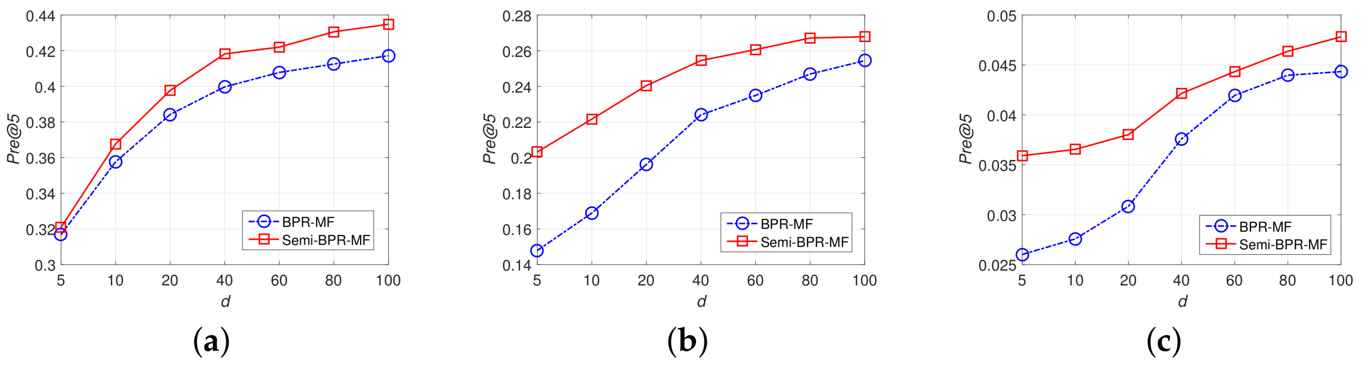
4.2. Impacts of Parameters

The purpose of this experiment was to investigate the impacts of different parameter settings on the performance of our approach.
A key step in our approach is splitting users’ unobserved feedback into two subsets: the intermediate item set (T) and the negative item set (N). The parameter r plays a very important role in the split, and it controls the proportion of items in the intermediate set. To study the impacts of different r values on the recommendation performance, we varied r from 0 to 1 . 0 . For each given r value, we adjusted the other parameters ( α , β and γ ) to achieve the best performance. In this experiment, the number of latent dimensions d was fixed at 100. Figure 4 shows the impact of r on the performance.
In the Movielens 1M and Ciao datasets, the metric Pre@5 gradually improves with the growth of parameter r, and the best performances are achieved when r approximates 0.1 for the Movielens 1M dataset and 0.4 for the Ciao dataset. If r continues to increase, the performance experiences a decrease. In the Lastfm 2K dataset, the peak performance is obtained when r is around 0.05, and the performance gradually deteriorates as r increases. In extreme cases, when r = 1 . 0 , which means we add all of the users’ unrated items into the intermediate set, our Semi-BPR model reduces to the standard BPR model.
Another important parameter in the Semi-BPR-MF model is the dimension of latent factors d. It controls the capability of the matrix factorization algorithm and, thus, may have an important effect on the recommendation performance. In this experiment, we chose the dimension of latent factors from {5, 10, 20, 40, 60, 80, 100}. For each given dimension d, we tuned the other parameters to achieve the optimal performance.
Figure 5 shows the recommendation quality with different dimensions of latent factors. It can be observed that the performances of BPR-MF and Semi-BPR-MF gradually improved with the increase of dimension d in all datasets. In addition, we can see that our Semi-BPR-MF model consistently outperformed the BPR-MF model in all cases, especially for the spare Lastfm 2K and Ciao datasets. Setting dimension d to 100 was shown to be the best choice for all datasets to balance the recommendation performance and computational complexity.

4.3. Performance Comparison

4.3.1. Baselines

In order to demonstrate the effectiveness of the proposed approach, we compared our model with several state-of-the-art baselines.
Most Popular (MostPop): This is a basic recommendation model, which ranks items according to their popularity and recommends popular items to each user. MostPop does not consider users’ preferences and, thus, cannot provide personalized recommendations.
Neighborhood approaches: User-based K-Nearest Neighbor (UserKNN) and Item-based K-Nearest Neighbor (ItemKNN) are two typical neighborhood-based models. UserKNN recommends items to each user that have been rated by similar users, while ItemKNN recommends items to each user that are similar to his/her rated items. For neighborhood approaches, the binary-cosine was adopted as the similarity measure.
Pointwise approaches: The Weighted Regularized Matrix Factorization (WRMF) is a state-of-the-art pointwise recommendation model [4]. WRMF treats the rating data as indications of positive and negative feedback associated with different confidence levels and learns model parameters by fitting the rating data.
Pairwise approaches: BPR is a generic optimization criterion for personalized recommendations. Matrix Factorization with BPR optimizations (BPR-MF) and K-Nearest Neighbor with BPR optimizations (BPR-KNN) are two representative pairwise recommendation models [7]. Our Semi-BPR-MF model is based on the BPR-MF model and also belongs to this category. For the pairwise approaches, 100 pairs were randomly sampled for each user in the training phase.

4.3.2. Parameter Settings

For each compared approach, we determined the optimal parameter settings through a grid search. The MostPop model has no parameters to be set. For the UserKNN model and ItemKNN model, the number of neighbors k n n was chosen from { 40 , 60 , 80 , 100 , 120 , 160 , 200 } . For the WRMF model, the weight ( α ) was chosen from { 0 , 1 , 5 , 10 } . For our Semi-BPR-MF model, we chose the proportion of the intermediate item set r from { 0 . 01 , 0 . 05 , 0 . 1 , 0 . 2 , 0 . 4 , 0 . 6 , 0 . 8 , 1 . 0 } and the weight coefficient parameters ( α , β , and γ ) from { 0 . 1 , 0 . 2 , 0 . 3 , 0 . 4 , 0 . 5 , 0 . 6 , 0 . 7 , 0 . 8 , 0 . 9 , 1 . 0 } . For all methods, the dimension of latent factors d was chosen from { 10 , 20 , 50 , 100 } , and the regularization coefficient ( λ ) was chosen from { 0 . 001 , 0 . 005 , 0 . 01 , 0 . 02 , 0 . 05 , 0 . 1 , 0 . 2 , 0 . 5 , 1 , 2 , 5 , 10 , 20 , 50 , 100 } . The optimal parameter settings are shown in Table 3.

4.3.3. Recommendation Performance

The top-N recommendation performances of the different approaches are shown in Table 4. From the experimental results, we can make the following conclusions:
  • MostPop was the worst of all compared approaches, which implies that generating personalized recommendations for each user is very necessary.
  • UserKNN, ItemKNN approaches are popular in recommender systems. Their performance depends on the choice of a heuristic similarity measure. In most cases, neighborhood approaches were shown to be worse than pointwise or pairwise approaches.
  • WRMF is the state-of-the-art pointwise approach for top-N recommendation tasks. However, WRMF cannot directly optimize the ranking-oriented metrics and is slightly worse than the BPR-MF pairwise approach. This demonstrates that pairwise assumptions are more reasonable than pointwise assumptions.
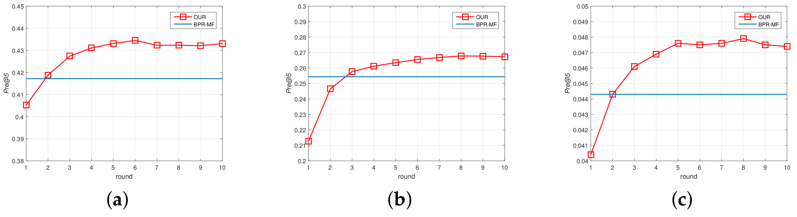
  • In all three datasets, the proposed Semi-BPR-MF model outperformed the other baselines in all evaluation metrics. For sparse datasets, like the Ciao dataset, only considering user preference between the observed feedback and unobserved feedback can not achieve a satisfactory level of performance. Compared with the best baseline BPR-MF model, our approach can obtain a significant performance improvement.
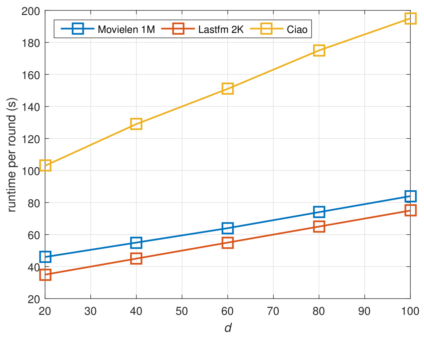
In the above experiments, the number of top-N items (N) was fixed at five. To compare the recommendation performances with different values of N, we varied N in the range [ 1 , 100 ] , and the results are shown in Figure 6. We found that our Semi-BPR-MF model performed best in all compared methods.

4.4. Scalability

In this experiment, we aimed to evaluate the scalability of the proposed approach. The dimension of latent factors d is a key factor that affects the computation complexity of our approach. As analyzed earlier, the computational complexity of Semi-BPR-MF is O ( d · S + m n ( d + l o g n ) ) . Figure 7 illustrates the runtime per self-training round on the Movielens 1M, Lastfm 2K and Ciao datasets. We observed that the runtime increased almost linearly with an increase in dimension d.
Figure 8 shows the convergence of our approach on all datasets. We found that our approach converged after about five self-training rounds and then fluctuated in a small range around the best performance.

5. Conclusions

In this paper, we proposed a semi-supervised model for top-N recommendation tasks. Based on the assumption that users always prefer items that are ranked higher in the recommendation list generated by a given model, we selected a certain number of items ranked higher in the recommendation list to construct an intermediate set and optimize the AUC metric. Our approach adopts the self-training paradigm to improve the recommendation performance iteratively. We conducted extensive experiments on three popular datasets to evaluate the effectiveness of the proposed approach. For future work, there are still several issues to be studied. A promising research direction is the integration of auxiliary information (e.g., description information of items, users’ reviews) into our model. In real environments, the user-item rating matrix is very sparse, and some new users or items only have very few rating data, that is the so-called cold-start problem. Therefore, it is worth studying the combination of the traditional recommendation model with semi-supervised learning to solve the cold-start problem.

Author Contributions

Y.P. proposed the research direction and gave the conceptualization. S.C. implemented the proposed approach, conducted experiments and wrote the paper.

Funding

This work was supported by The National Key Research and Development Program of China (2016 YFB1000100).

Conflicts of Interest

The authors declare that there is no conflict of interest regarding the publication of this article.

References

  1. Bell, R.M.; Koren, Y. Lessons from the netflix prize challenge. ACM SIGKDD Explor. Newsl. 2007, 9, 75–79. [Google Scholar] [CrossRef]
  2. Linden, G.; Smith, B.; York, J. Amazon.com recommendations: Item-to-item collaborative filtering. IEEE Int. Comput. 2003, 7, 76–80. [Google Scholar] [CrossRef]
  3. Pan, R.; Zhou, Y.; Cao, B.; Liu, N.; Lukose, R.; Scholz, M.; Yang, Q. One-class collaborative filtering. In Proceedings of the 2008 8th IEEE International Conference on Data Mining, Pisa, Italy, 15–19 December 2008; pp. 502–511. [Google Scholar]
  4. Hu, Y.; Koren, Y.; Volinsky, C. Collaborative filtering for implicit feedback datasets. In Proceedings of the 2008 8th IEEE International Conference on Data Mining, Pisa, Italy, 15–19 December 2008; pp. 263–272. [Google Scholar]
  5. Ning, X.; Karypis, G. SLIM: Sparse linear methods for top-N recommender systems. In Proceedings of the 2011 11th IEEE International Conference on Data Mining, Vancouver, BC, Canada, 11–14 December 2011; pp. 497–506. [Google Scholar]
  6. Kabbur, S.; Ning, X.; Karypis, G. FISM: Factored item similarity models for top-n recommender systems. In Proceedings of the 19th ACM SIGKDD International Conference on Knowledge Discovery & Data Mining, Chicago, IL, USA, 11–14 August 2013; pp. 659–667. [Google Scholar]
  7. Rendle, S.; Freudenthaler, C.; Gantner, Z.; Schmidt-Thieme, L. BPR: Bayesian personalized ranking from implicit feedback. In Proceedings of the 23th Conference on Uncertainty in Artificial Intelligence (UAI 2009), Montreal, QC, Cananda, 18–21 June 2009; pp. 452–461. [Google Scholar]
  8. Pan, W.; Chen, L. GBPR: Group preference based bayesian personalized ranking for one-class collaborative filtering. In Proceedings of the 23th International Joint Conference on Artificial Intelligence, Beijing, China, 3–9 August 2013; pp. 2691–2697. [Google Scholar]
  9. Shi, Y.; Karatzoglou, A.; Baltrunas, L.; Larson, M.; Oliver, N.; Hanjalic, A. CLiMF: Collaborative less-is-more filtering. In Proceedings of the 23th International Joint Conference on Artificial Intelligence, Beijing, China, 3–9 August 2013; pp. 3077–3081. [Google Scholar]
  10. Shi, Y.; Karatzoglou, A.; Baltrunas, L.; Larson, M.; Hanjalic, A.; Oliver, N. TFMAP: Optimizing map for top-n context-aware recommendation. In Proceedings of the 35th ACM Special Interest Group on Information Retrieval (SIGIR), Portland, OR, USA, 12–16 August 2012; pp. 155–164. [Google Scholar]
  11. Zhao, T.; Mcauley, J.; King, I. Leveraging social connections to improve personalized ranking for collaborative filtering. In Proceedings of the 23th ACM International Conference on Conference on Information and Knowledge Management, Shanghai, China, 3–7 November 2014; pp. 261–270. [Google Scholar]
  12. Song, D.; Meyer, D.A. Recommending positive links in signed social networks by optimizing a generalized AUC. In Proceedings of the 29th AAAI Conference on Artificial Intelligence, Austin, TX, USA, 25–30 January 2015; pp. 290–296. [Google Scholar]
  13. Liu, H.; Wu, Z.; Zhang, X. CPLR: Collaborative pairwise learning to rank for personalized recommendation. Knowl.-Based Syst. 2018, 148, 31–40. [Google Scholar] [CrossRef]
  14. Yu, L.; Zhang, C.; Pei, S.; Sun, G.; Zhang, X. Walkranker: A unified pairwise ranking model with multiple relations for item recommendation. In Proceedings of the 32th AAAI Conference on Artificial Intelligence, New Orleans, LA, USA, 2–7 February 2018. [Google Scholar]
  15. Hady, M.F.A.; Schwenker, F. Semi-supervised learning. J. R. Stat. Soc. 2006, 172, 530. [Google Scholar]
  16. Zhang, M.; Tang, J.; Zhang, X.; Xue, X. Addressing cold start in recommender systems: a semi-supervised co-training algorithm. In Proceedings of the 37th International ACM SIGIR Conference on Research & Development in Information Retrieval, Gold Coast, Australia, 6–11 July 2014; pp. 73–82. [Google Scholar]
  17. Zhang, X. Utilizing tri-training algorithm to solve cold start problem in recommender system. Comput. Sci. 2016, 12, 108–114. [Google Scholar]
  18. Hao, Z.; Cheng, Y.; Cai, R.; Wen, W.; Wang, L. A semi-supervised solution for cold start issue on recommender systems. In Proceedings of the Asia-Pacific Web Conference, Guangzhou, China, 18–20 September 2015; pp. 805–817. [Google Scholar]
  19. Usunier, N.; Amini, M.R.; Goutte, C. Multiview Semi-supervised Learning for Ranking Multilingual Documents. In Proceedings of the Joint European Conference on Machine Learning and Knowledge Discovery in Databases, Athens, Greece, 4–8 September 2011. [Google Scholar]
  20. Truong, T.V.; Amini, M.R.; Gallinari, P. A self-training method for learning to rank with unlabeled data. In Proceedings of the European Symposium on Artificial Neural Networks–Advances in Computational Intelligence and Learning, Bruges, Belgium, 22–24 April 2009. [Google Scholar]
  21. Koren, Y.; Bell, R.; Volinsky, C. Matrix factorization techniques for recommender systems. IEEE Comput. J. 2009, 42, 30–37. [Google Scholar] [CrossRef]
  22. Guo, G.; Zhang, J.; Sun, Z.; Yorke-Smith, N. Librec: A java library for recommender systems. In Proceedings of the 23th Conference on User Modeling, Posters, Demos, Late-breaking Results and Workshop Adaptation and Personalization (UMAP 2015), Dublin, Ireland, 29 June–3 July 2015. [Google Scholar]
Figure 1. Average hit rate at different positions of the recommendation list.
Symmetry 10 00492 g001
Figure 2. Overview of our approach.
Symmetry 10 00492 g002
Figure 3. A case study on a user. MF, Matrix Factorization.
Symmetry 10 00492 g003
Figure 4. Impact of parameter r on the recommendation performance. (a) Impact of r on Movielens 1M dataset; (b) Impact of r on Lastfm 2K dataset; (c) Impact of r on Ciao dataset.
Symmetry 10 00492 g004
Figure 5. Recommendation performance with different dimensions d. (a) Recommendation performance variation on Movielens 1M dataset; (b) Recommendation performance variation on Lastfm 2K dataset; (c) Recommendation performance variation on Ciao dataset.
Symmetry 10 00492 g005
Figure 6. Performance comparison for different values of N. (a) Performance comparison on Movielens 1M dataset; (b) Performance comparison on Lastfm 2K dataset; (c) Performance comparison on Ciao dataset.
Symmetry 10 00492 g006
Figure 7. Runtime per self-training round.
Symmetry 10 00492 g007
Figure 8. Convergence of our approach. (a) Convergence on Movielens 1M dataset; (b) Convergence on Lastfm 2K dataset; (c) Convergence on Ciao dataset.
Symmetry 10 00492 g008
Table 1. Summary of symbols used in this paper.
SymbolDescription
UUser set
IItem set
m = | U | User number
n = | I | Item number
u U Used to index a user
i , j , k I Used to index an item
U i Users that have rated item i
I u Items that user u has rated
R m × n Rating matrix. R u , i = 1 , if the feedback is observed; otherwise, R u , i = 0 .
f u The scoring function of user u. f u ( i ) refers to the predicted scoring value of item i.
Table 2. Dataset statistics.
DatasetUser#Item#Feedback#Density
Movielens 1M604037061,000,2094.47%
Lastfm 2K189217,63292,8340.28%
Ciao726711,211147,9870.18%
Table 3. Parameter settings of different methods.
MethodMovielens 1MLastfm 2KCiao
MostPop---
UserKNN k n n = 200 k n n = 100 k n n = 100
ItemKNN k n n = 120 k n n = 80 k n n = 100
WRMF d = 50 , α = 1 , d = 50 , α = 1 , d = 50 , α = 5 ,
λ U = λ I = 5 λ U = λ I = 10 λ U = λ I = 100 ,
BPR-MF d = 100 , d = 100 , d = 100 ,
λ U = λ I = 0 . 01 , λ b = 0 . 005 λ U = λ I = λ b = 0 . 005 λ U = λ I = λ b = 0 . 02
BPR-KNN λ = 0 . 01 λ = 0 . 01 λ = 10
Semi-BPR-MF d = 100 , r = 0.1, d = 100 , r = 0 . 05 , d = 100 , r = 0 . 4 ,
λ U = λ I = λ b = 0 . 02 , λ U = λ I = λ b = 0 . 01 , λ U = λ I = 0 . 02 , λ b = 0 . 01 ,
α = 0 . 5 , β = 0 . 2 , γ = 0 . 4 α = 1 , β = 0 . 1 , γ = 0 . 1 α = 0 . 3 , β = 0 . 4 , γ = 0 . 6
Table 4. Recommendation performances of different models. The best results are highlighted in bold font and the best baseline results are underlined.
DatasetModelsPre@5Rec@5MAP@5MRR@5AUC@5NDCG@5
MostPop0.20880.04050.14990.35250.76260.2181
UserKNN0.38950.09820.30870.60880.89750.4118
ItemKNN0.33110.07720.25790.53900.86240.3514
Movielens 1MWRMF0.41380.10590.32920.63300.90920.4359
BPR-KNN0.40180.10020.32230.61660.90050.4245
BPR-MF0.41720.10320.33820.62620.90550.4387
Semi-BPR-MF0.43450.10800.35600.64640.91290.4571
MostPop0.08570.04480.05670.18880.64580.0952
UserKNN0.20020.10440.15420.42330.78480.2300
ItemKNN0.23730.12340.18440.48970.82460.2714
Lastfm 2KWRMF0.24580.12780.18230.48070.83650.2727
BPR-KNN0.24590.12630.18360.49100.83810.2750
BPR-MF0.25440.13120.18860.49480.84690.2813
Semi-BPR-MF0.26780.13870.20750.52300.85090.3007
MostPop0.02810.02890.02510.06650.55330.0385
UserKNN0.04220.04210.03690.09630.57670.0562
ItemKNN0.03620.03250.02940.07720.56420.0453
CiaoWRMF0.04480.04330.03650.09720.58170.0573
BPR-KNN0.04250.04150.03510.09420.57900.0551
BPR-MF0.04430.04660.03830.10130.58470.0594
Semi-BPR-MF0.04780.05060.04150.10950.59080.0642

