Statistical Inference for the Information Entropy of the Log-Logistic Distribution under Progressive Type-I Interval Censoring Schemes


Abstract
1. Introduction
2. Information Entropy
- (1)
- Indicating the average amount of information provided by each message or symbol after the source is output;
- (2)
- Indicating the average uncertainty of the source after the source is output;
- (3)
- Measuring the uncertainty on a random variable T.
3. Parameter Estimations
3.1. Maximum Likelihood Estimation
3.2. EM Algorithm
- Step E: Find the conditional distribution of or with respect to Z, i.e.,
- Step M: Maximize , that is find a point to make .
- Step E: According to the concept of the likelihood function:
- Step M: Deriving with respect to to find the maximum point of :Let ; can be calculated as:Let , and replace with , then can be defined as:
4. Hypothesis Testing Algorithm
- (i)
- The estimation of the (conditional) entropy or mutual information can be applied to independent component analysis in order to measure the dependency among random variables (see [16]).
- (ii)
- A discretization algorithm for continuous features and attributes of a raw and rough set for selecting cut points can be illustrated on the basis of information entropy, which is defined for every candidate cut point and treated as a measurement of importance (see [17]).
- (iii)
- The information entropy can be applied in a multi-population genetic algorithm used to narrow the search space. By defining the probabilities that the best solution appears in each population, information-entropy is introduced into the evolution process, which will enhance the ability of searching optimization solution for the evolution algorithms (see [18]).
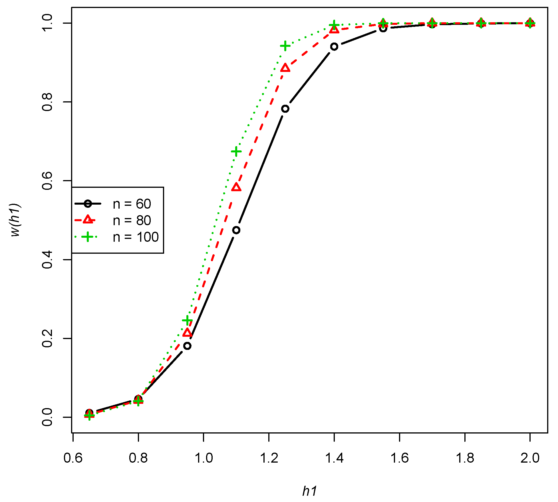
- For , and , the power function presents a non-decreasing trend with respect to n, as performed in Figure 1 (any combinations of m, p and will have the same trend).
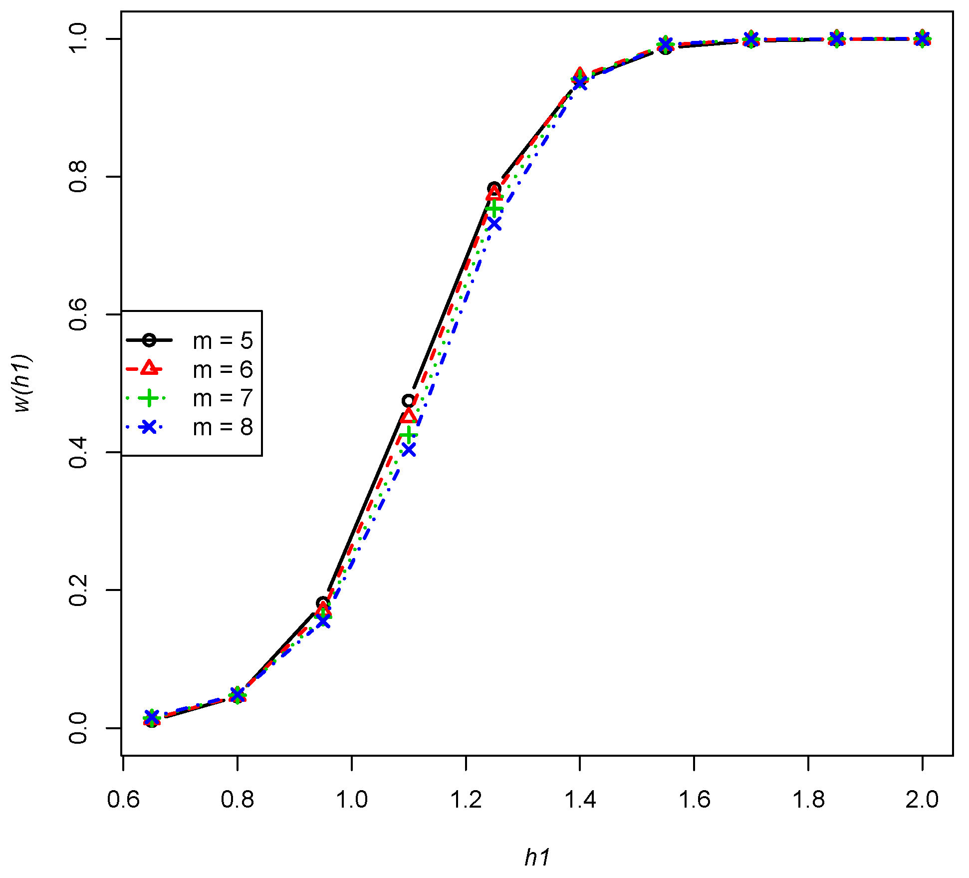
- The power is a fixed non-increasing function of m, , , , as performed in Figure 2 (any combinations of n, and p will have a similar trend).
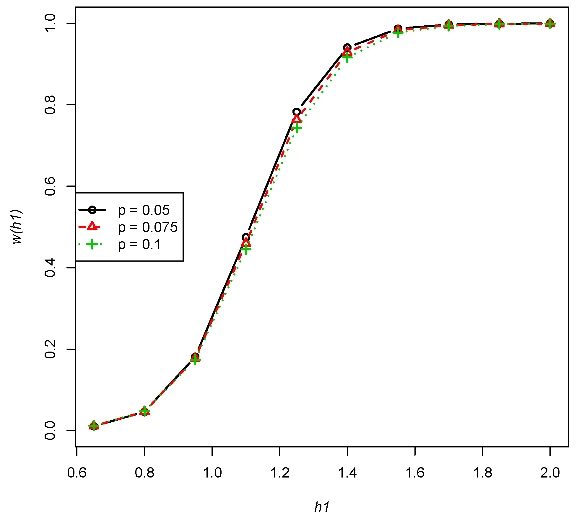
- The power function presents a non-increasing trend of the fixed deleted percentage p of , , , as performed in Figure 3 (any combinations of n, m and will have a similar trend).
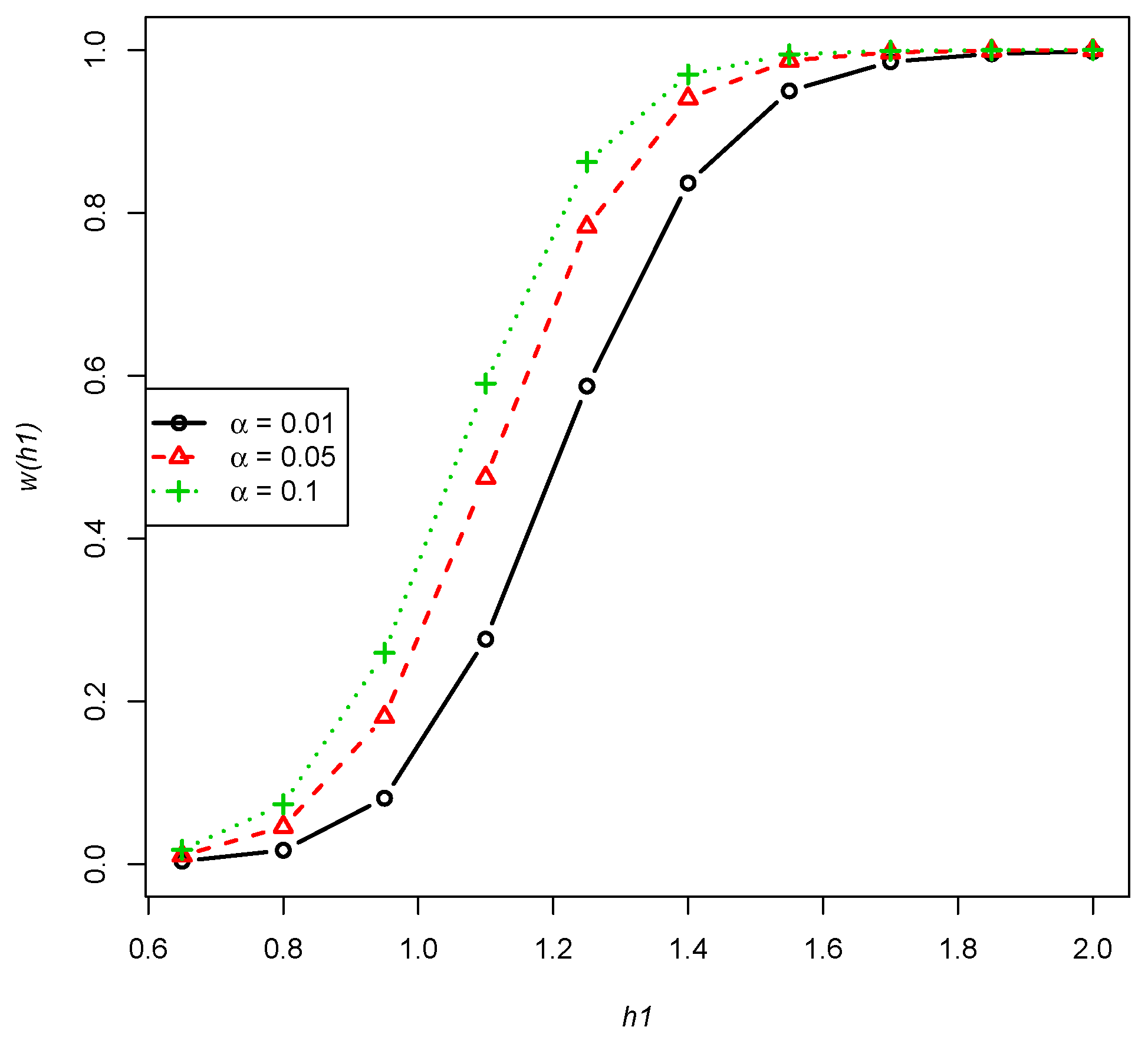
- From Figure 4, for any combination of n, m and p, the power function presents a non-decreasing trend with respect to .
- Step 1
- Observe the progressive type-I interval censored data at the pre-scheduled times with censoring schemes of from the log-logistic distribution.
- Step 2
- In practical applications, h represents the critical amount of information required to reduce the source input to a certain standard. Then, the testing null hypothesis and the alternative hypothesis are constructed.
- Step 3
- Calculate the maximum likelihood estimate of and the value of the test statistic .
- Step 4
- The critical value can be calculated for the level of significance of as:
- Step 5
- Compare the size of and . Determine whether the obtained source data meet the requirements.
5. Monte Carlo Simulation
- Step 1
- Observe the progressive type-I interval censored data at the pre-set times with the censoring schemes of.
- Step 2
- Let the critical amount of information required , and then, propose the test null hypothesis and the alternative hypothesis .
- Step 3
- Calculate the maximum likelihood estimate of parameter and the value of the test statistic .
- Step 4
- The critical value can be calculated for the level of significance of as: .
- Step 5
- Since , we accept the null hypothesis . Thus, the obtained source data do not meet the requirements.
- Step 1
- Record the progressive type-I interval censored sample at the pre-set times with the censoring scheme of .
- Step 2
- If the critical amount of information required , then, we can propose the test null hypothesis and the alternative hypothesis .
- Step 3
- Calculate the maximum likelihood estimate of parameter and the value of the test statistic .
- Step 4
- The critical value can be calculated for the level of significance of as: .
- Step 5
- Since , we accept the null hypothesis . Thus, the obtained source data do not meet the requirements.
6. Conclusions
Author Contributions
Funding
Conflicts of Interest
References
- Shah, B.K.; Dave, P.H. A note on log-logistic distribution. J. MS Univ. Baroda 1963, 12, 15–20. [Google Scholar]
- Tadikamalla, P.R.; Johnson, N.L. Tables to facilitate fitting lu distributions. Commun. Stat. Simul. Comput. 1982, 11, 249–271. [Google Scholar] [CrossRef]
- O’Quigley, J.; Struthers, L. Survival models based upon the logistic and log–logistic distributions. Comput. Progr. Biomed. 1982, 15, 3–11. [Google Scholar] [CrossRef]
- Balakrishnan, N.; Malik, H.J. Moments of order statistics from truncated log-logistic distribution. J. Stat. Plan. Inference 1987, 17, 251–267. [Google Scholar] [CrossRef]
- Kantam, R.R.L.; Rosaiah, K.; Rao, G.S. Acceptance sampling based on life tests: Log-logistic model. J. Appl. Stat. 2001, 28, 121–128. [Google Scholar] [CrossRef]
- Chen, D.G.; Lio, Y.L.; Jiang, N. Lower confidence limits on the generalized exponential distribution percentiles under progressive type-i interval censoring. Commun. Stat. Simul. Comput. 2013, 42, 2106–2117. [Google Scholar] [CrossRef]
- Singh, S.; Tripathi, Y.M. Estimating the parameters of an inverse weibull distribution under progressive type-i interval censoring. Stat. Pap. 2016, 59, 21–56. [Google Scholar] [CrossRef]
- Wu, S.F.; Lin, Y.T.; Chang, W.J.; Chang, C.W.; Lin, C. A computational algorithm for the evaluation on the lifetime performance index of products with rayleigh distribution under progressive type i interval censoring. J. Comput. Appl. Math. 2017, 328, 508–519. [Google Scholar] [CrossRef]
- Wu, S.J.; Huang, S.R. Planning progressive type-i interval censoring life tests with competing risks. IEEE Trans. Reliab. 2014, 63, 511–522. [Google Scholar] [CrossRef]
- Basak, I.; Balakrishnan, N. Prediction of censored exponential lifetimes in a simple step-stress model under progressive type ii censoring. Comput. Stat. 2017, 32, 1–23. [Google Scholar] [CrossRef]
- El-Sagheer, R.M. Inferences in constant-partially accelerated life tests based on progressive type-ii censoring. Bull. Malays. Math. Sci. Soc. 2016, 41, 609–626. [Google Scholar] [CrossRef]
- Singh, S.K.; Singh, U.; Kumar, M. Bayesian estimation for poisson-exponential model under progressive type-ii censoring data with binomial removal and its application to ovarian cancer data. Commun. Stat. Simul. Comput. 2014, 45, 3457–3475. [Google Scholar] [CrossRef]
- Aggarwala, R. Progressive interval censoring: Some mathematical results with applications to inference. Commun. Stat. 2001, 30, 1921–1935. [Google Scholar] [CrossRef]
- Liu, H. Asymptotic normality of maximum likelihood estimators for truncated and censored data. J. Huzhou Teach. Coll. 1996, 5, 17–22. [Google Scholar]
- Mao, S.; Wang, J.; Pu, X. Advanced Mathematical Statistics; Higher Education Press: Beijing, China, 2006. [Google Scholar]
- Zhong, N.; Deng, X. Multimode non-Gaussian process monitoring based on local entropy independent component analysis. Can. J. Chem. Eng. 2017, 95, 319–330. [Google Scholar] [CrossRef]
- Xie, H.; Cheng, H.Z.; Niu, D.X. Discretization of continuous attributes in rough set theory based on information entropy. Chin. J. Comput. 2005, 28, 1570. [Google Scholar]
- Li, C.L.; Wang, X.C.; Zhao, J.C. An information entropy-based multi-population genetic algorithm. J. Dalian Univ. Technol. 2004, 44, 589–593. [Google Scholar]
- Fishman, G.S. A Monte Carlo sampling plan for estimating network reliability. Oper. Res. 2017, 34, 581–594. [Google Scholar] [CrossRef]
- Blevins, J.R. Sequential Monte Carlo Methods for Estimating Dynamic Microeconomic Models. J. Appl. Econom. 2011, 31, 773–804. [Google Scholar] [CrossRef]
- Graham, I.G.; Scheichl, R.; Ullmann, E. Mixed finite element analysis of lognormal diffusion and multilevel Monte Carlo methods. Stoch. Part. Differ. Equ. Anal. Comput. 2016, 4, 41–75. [Google Scholar] [CrossRef]


| m | n | p | 0.65 | 0.8 | 0.95 | 1.1 | 1.25 | 1.4 | 1.55 | 1.7 | 1.85 | 2 |
|---|---|---|---|---|---|---|---|---|---|---|---|---|
| 5 | 60 | 0.05 | 0.003800 | 0.017245 | 0.081148 | 0.276383 | 0.587226 | 0.836528 | 0.949660 | 0.985413 | 0.995253 | 0.998054 |
| 0.075 | 0.004032 | 0.017650 | 0.079868 | 0.265915 | 0.564973 | 0.815618 | 0.937988 | 0.980286 | 0.993032 | 0.996955 | ||
| 0.1 | 0.004284 | 0.018076 | 0.078677 | 0.255964 | 0.543147 | 0.793769 | 0.924717 | 0.973913 | 0.990040 | 0.995381 | ||
| 80 | 0.05 | 0.002183 | 0.015033 | 0.095768 | 0.363243 | 0.729005 | 0.932958 | 0.988235 | 0.998036 | 0.999598 | 0.999882 | |
| 0.075 | 0.002336 | 0.015356 | 0.093514 | 0.347988 | 0.705013 | 0.918962 | 0.983776 | 0.996901 | 0.999286 | 0.999771 | ||
| 0.1 | 0.002504 | 0.015695 | 0.091385 | 0.333371 | 0.680742 | 0.903316 | 0.978118 | 0.995260 | 0.998781 | 0.999575 | ||
| 100 | 0.05 | 0.001342 | 0.013628 | 0.112273 | 0.451078 | 0.832886 | 0.975445 | 0.997651 | 0.999781 | 0.999972 | 0.999994 | |
| 0.075 | 0.001449 | 0.013899 | 0.108974 | 0.431713 | 0.811215 | 0.967936 | 0.996335 | 0.999592 | 0.999940 | 0.999986 | ||
| 0.1 | 0.001566 | 0.014185 | 0.105847 | 0.412975 | 0.788483 | 0.958886 | 0.994453 | 0.999270 | 0.999876 | 0.999968 | ||
| 6 | 60 | 0.05 | 0.004883 | 0.017812 | 0.074107 | 0.250705 | 0.561279 | 0.833421 | 0.956602 | 0.990605 | 0.997878 | 0.999399 |
| 0.075 | 0.005045 | 0.018186 | 0.073611 | 0.243013 | 0.540752 | 0.811918 | 0.945089 | 0.986392 | 0.996484 | 0.998884 | ||
| 0.1 | 0.005230 | 0.018583 | 0.073132 | 0.235600 | 0.520662 | 0.789520 | 0.931792 | 0.980875 | 0.994414 | 0.998031 | ||
| 80 | 0.05 | 0.002900 | 0.015485 | 0.087078 | 0.334081 | 0.710792 | 0.935323 | 0.991557 | 0.999122 | 0.999898 | 0.999983 | |
| 0.075 | 0.003011 | 0.015783 | 0.085822 | 0.321862 | 0.687350 | 0.921040 | 0.987709 | 0.998435 | 0.999778 | 0.999956 | ||
| 0.1 | 0.003137 | 0.016098 | 0.084597 | 0.310052 | 0.663750 | 0.905018 | 0.982626 | 0.997337 | 0.999549 | 0.999896 | ||
| 100 | 0.05 | 0.001839 | 0.014008 | 0.101885 | 0.420290 | 0.822110 | 0.978050 | 0.998653 | 0.999936 | 0.999996 | 1.000000 | |
| 0.075 | 0.001918 | 0.014258 | 0.099808 | 0.403906 | 0.800241 | 0.970707 | 0.997707 | 0.999857 | 0.999989 | 0.999999 | ||
| 0.1 | 0.002010 | 0.014524 | 0.097781 | 0.387973 | 0.777431 | 0.961735 | 0.996257 | 0.999700 | 0.999971 | 0.999996 | ||
| 7 | 60 | 0.05 | 0.005761 | 0.018483 | 0.069396 | 0.227948 | 0.527358 | 0.817161 | 0.955804 | 0.992186 | 0.998704 | 0.999743 |
| 0.075 | 0.005817 | 0.018796 | 0.069612 | 0.223634 | 0.511146 | 0.796710 | 0.944284 | 0.988356 | 0.997680 | 0.999455 | ||
| 0.1 | 0.005910 | 0.019137 | 0.069752 | 0.219159 | 0.494940 | 0.775408 | 0.930965 | 0.983214 | 0.996057 | 0.998920 | ||
| 80 | 0.05 | 0.003498 | 0.016019 | 0.080815 | 0.305489 | 0.680614 | 0.928605 | 0.992033 | 0.999417 | 0.999959 | 0.999996 | |
| 0.075 | 0.003538 | 0.016268 | 0.080510 | 0.297471 | 0.660316 | 0.914282 | 0.988308 | 0.998892 | 0.999897 | 0.999987 | ||
| 0.1 | 0.003603 | 0.016539 | 0.080111 | 0.289328 | 0.639687 | 0.898304 | 0.983342 | 0.998005 | 0.999762 | 0.999963 | ||
| 100 | 0.05 | 0.002264 | 0.014457 | 0.093988 | 0.387302 | 0.798857 | 0.975914 | 0.998856 | 0.999968 | 0.999999 | 1.000000 | |
| 0.075 | 0.002295 | 0.014667 | 0.093118 | 0.375615 | 0.778690 | 0.968368 | 0.998005 | 0.999920 | 0.999997 | 1.000000 | ||
| 0.1 | 0.002343 | 0.014894 | 0.092138 | 0.363819 | 0.757631 | 0.959218 | 0.996669 | 0.999815 | 0.999989 | 0.999999 | ||
| 8 | 60 | 0.05 | 0.006372 | 0.019094 | 0.066647 | 0.211436 | 0.496750 | 0.797345 | 0.952000 | 0.992552 | 0.999033 | 0.999861 |
| 0.075 | 0.006325 | 0.019329 | 0.067386 | 0.210105 | 0.485710 | 0.779344 | 0.940671 | 0.988891 | 0.998195 | 0.999674 | ||
| 0.1 | 0.006334 | 0.019602 | 0.067964 | 0.208126 | 0.473880 | 0.760275 | 0.927569 | 0.983926 | 0.996808 | 0.999297 | ||
| 80 | 0.05 | 0.003922 | 0.016505 | 0.076893 | 0.283451 | 0.650493 | 0.918498 | 0.991494 | 0.999511 | 0.999977 | 0.999999 | |
| 0.075 | 0.003890 | 0.016692 | 0.077317 | 0.279394 | 0.634761 | 0.904809 | 0.987749 | 0.999051 | 0.999937 | 0.999995 | ||
| 0.1 | 0.003897 | 0.016909 | 0.077527 | 0.274567 | 0.618106 | 0.889515 | 0.982776 | 0.998255 | 0.999843 | 0.999983 | ||
| 100 | 0.05 | 0.002571 | 0.014865 | 0.088823 | 0.360549 | 0.773440 | 0.971817 | 0.998821 | 0.999977 | 1.000000 | 1.000000 | |
| 0.075 | 0.002549 | 0.015023 | 0.088903 | 0.353590 | 0.756498 | 0.964200 | 0.997973 | 0.999940 | 0.999999 | 1.000000 | ||
| 0.1 | 0.002556 | 0.015204 | 0.088720 | 0.345768 | 0.738370 | 0.955043 | 0.996647 | 0.999855 | 0.999994 | 1.000000 |
| m | n | p | 0.65 | 0.8 | 0.95 | 1.1 | 1.25 | 1.4 | 1.55 | 1.7 | 1.85 | 2 |
|---|---|---|---|---|---|---|---|---|---|---|---|---|
| 5 | 60 | 0.05 | 0.010636 | 0.046060 | 0.181003 | 0.474751 | 0.782816 | 0.940493 | 0.986955 | 0.997095 | 0.999202 | 0.999697 |
| 0.075 | 0.011153 | 0.046622 | 0.177388 | 0.459489 | 0.763251 | 0.928988 | 0.982639 | 0.995690 | 0.998700 | 0.999472 | ||
| 0.1 | 0.011703 | 0.047209 | 0.173927 | 0.444650 | 0.743263 | 0.916199 | 0.977317 | 0.993767 | 0.997949 | 0.999112 | ||
| 80 | 0.05 | 0.006827 | 0.042893 | 0.212941 | 0.581850 | 0.884698 | 0.982370 | 0.997991 | 0.999758 | 0.999960 | 0.999989 | |
| 0.075 | 0.007220 | 0.043365 | 0.207659 | 0.563229 | 0.868646 | 0.977054 | 0.996940 | 0.999570 | 0.999918 | 0.999976 | ||
| 0.1 | 0.007639 | 0.043859 | 0.202583 | 0.544881 | 0.851533 | 0.970624 | 0.995462 | 0.999264 | 0.999842 | 0.999949 | ||
| 100 | 0.05 | 0.004598 | 0.040788 | 0.245816 | 0.674392 | 0.942291 | 0.995271 | 0.999729 | 0.999983 | 0.999998 | 1.000000 | |
| 0.075 | 0.004902 | 0.041201 | 0.238886 | 0.654207 | 0.931014 | 0.993245 | 0.999524 | 0.999963 | 0.999996 | 0.999999 | ||
| 0.1 | 0.005228 | 0.041633 | 0.232212 | 0.634008 | 0.918416 | 0.990560 | 0.999193 | 0.999924 | 0.999990 | 0.999998 | ||
| 6 | 60 | 0.05 | 0.012925 | 0.046845 | 0.169828 | 0.451170 | 0.773750 | 0.945074 | 0.990947 | 0.998680 | 0.999777 | 0.999947 |
| 0.075 | 0.013271 | 0.047359 | 0.167452 | 0.438091 | 0.754239 | 0.933478 | 0.987263 | 0.997804 | 0.999564 | 0.999881 | ||
| 0.1 | 0.013660 | 0.047900 | 0.165119 | 0.425308 | 0.734376 | 0.920492 | 0.982529 | 0.996487 | 0.999194 | 0.999753 | ||
| 80 | 0.05 | 0.008534 | 0.043553 | 0.199632 | 0.559181 | 0.881627 | 0.985367 | 0.998941 | 0.999933 | 0.999995 | 0.999999 | |
| 0.075 | 0.008808 | 0.043985 | 0.195841 | 0.542395 | 0.865285 | 0.980369 | 0.998228 | 0.999857 | 0.999985 | 0.999998 | ||
| 0.1 | 0.009114 | 0.044439 | 0.192121 | 0.525822 | 0.847913 | 0.974197 | 0.997145 | 0.999713 | 0.999964 | 0.999993 | ||
| 100 | 0.05 | 0.005900 | 0.041366 | 0.230547 | 0.654074 | 0.942088 | 0.996545 | 0.999896 | 0.999997 | 1.000000 | 1.000000 | |
| 0.075 | 0.006120 | 0.041743 | 0.225333 | 0.635237 | 0.930590 | 0.994819 | 0.999790 | 0.999992 | 1.000000 | 1.000000 | ||
| 0.1 | 0.006367 | 0.042140 | 0.220219 | 0.616397 | 0.917752 | 0.992446 | 0.999597 | 0.999980 | 0.999999 | 1.000000 | ||
| 7 | 60 | 0.05 | 0.014708 | 0.047764 | 0.161024 | 0.425370 | 0.753648 | 0.941871 | 0.991909 | 0.999150 | 0.999907 | 0.999986 |
| 0.075 | 0.014830 | 0.048189 | 0.159959 | 0.415859 | 0.736027 | 0.930271 | 0.988426 | 0.998486 | 0.999793 | 0.999962 | ||
| 0.1 | 0.015025 | 0.048649 | 0.158767 | 0.406226 | 0.717977 | 0.917311 | 0.983883 | 0.997431 | 0.999569 | 0.999905 | ||
| 80 | 0.05 | 0.009903 | 0.044324 | 0.188439 | 0.531179 | 0.868523 | 0.984874 | 0.999179 | 0.999969 | 0.999999 | 1.000000 | |
| 0.075 | 0.010008 | 0.044681 | 0.186311 | 0.518031 | 0.852898 | 0.979833 | 0.998572 | 0.999926 | 0.999996 | 1.000000 | ||
| 0.1 | 0.010168 | 0.045067 | 0.184040 | 0.504721 | 0.836307 | 0.973619 | 0.997619 | 0.999834 | 0.999987 | 0.999999 | ||
| 100 | 0.05 | 0.006973 | 0.042040 | 0.217055 | 0.626106 | 0.934584 | 0.996556 | 0.999932 | 0.999999 | 1.000000 | 1.000000 | |
| 0.075 | 0.007064 | 0.042352 | 0.213841 | 0.610595 | 0.923141 | 0.994839 | 0.999853 | 0.999997 | 1.000000 | 1.000000 | ||
| 0.1 | 0.007198 | 0.042689 | 0.210472 | 0.594800 | 0.910443 | 0.992476 | 0.999702 | 0.999991 | 1.000000 | 1.000000 | ||
| 8 | 60 | 0.05 | 0.015915 | 0.048590 | 0.155104 | 0.404095 | 0.732049 | 0.935697 | 0.991801 | 0.999320 | 0.999949 | 0.999995 |
| 0.075 | 0.015833 | 0.048906 | 0.155119 | 0.398271 | 0.717478 | 0.924473 | 0.988366 | 0.998752 | 0.999874 | 0.999984 | ||
| 0.1 | 0.015859 | 0.049270 | 0.154831 | 0.391745 | 0.702122 | 0.911917 | 0.983877 | 0.997818 | 0.999716 | 0.999954 | ||
| 80 | 0.05 | 0.010848 | 0.045018 | 0.180545 | 0.506603 | 0.852691 | 0.982997 | 0.999216 | 0.999980 | 1.000000 | 1.000000 | |
| 0.075 | 0.010793 | 0.045283 | 0.179838 | 0.497552 | 0.838775 | 0.977893 | 0.998636 | 0.999949 | 0.999998 | 1.000000 | ||
| 0.1 | 0.010823 | 0.045588 | 0.178759 | 0.487726 | 0.823790 | 0.971646 | 0.997719 | 0.999878 | 0.999994 | 1.000000 | ||
| 100 | 0.05 | 0.007728 | 0.042646 | 0.207223 | 0.600230 | 0.924505 | 0.996092 | 0.999940 | 1.000000 | 1.000000 | 1.000000 | |
| 0.075 | 0.007692 | 0.042878 | 0.205765 | 0.588809 | 0.913737 | 0.994305 | 0.999869 | 0.999998 | 1.000000 | 1.000000 | ||
| 0.1 | 0.007722 | 0.043144 | 0.203870 | 0.576536 | 0.901746 | 0.991875 | 0.999730 | 0.999995 | 1.000000 | 1.000000 |
| m | n | p | 0.65 | 0.8 | 0.95 | 1.1 | 1.25 | 1.4 | 1.55 | 1.7 | 1.85 | 2 |
|---|---|---|---|---|---|---|---|---|---|---|---|---|
| 5 | 60 | 0.05 | 0.017792 | 0.073840 | 0.259702 | 0.590335 | 0.862265 | 0.969759 | 0.994548 | 0.998951 | 0.999736 | 0.999903 |
| 0.075 | 0.018563 | 0.074431 | 0.254462 | 0.574080 | 0.846532 | 0.962638 | 0.992401 | 0.998355 | 0.999543 | 0.999821 | ||
| 0.1 | 0.019376 | 0.075048 | 0.249400 | 0.558055 | 0.830049 | 0.954421 | 0.989623 | 0.997493 | 0.999237 | 0.999679 | ||
| 80 | 0.05 | 0.012008 | 0.070473 | 0.302042 | 0.694889 | 0.935704 | 0.992577 | 0.999337 | 0.999933 | 0.999990 | 0.999997 | |
| 0.075 | 0.012631 | 0.070979 | 0.294897 | 0.676950 | 0.924651 | 0.989905 | 0.998930 | 0.999873 | 0.999978 | 0.999994 | ||
| 0.1 | 0.013290 | 0.071506 | 0.287976 | 0.658967 | 0.912494 | 0.986519 | 0.998322 | 0.999767 | 0.999954 | 0.999986 | ||
| 100 | 0.05 | 0.008430 | 0.068202 | 0.343607 | 0.777338 | 0.971524 | 0.998330 | 0.999928 | 0.999996 | 1.000000 | 1.000000 | |
| 0.075 | 0.008936 | 0.068650 | 0.334695 | 0.759552 | 0.964778 | 0.997486 | 0.999865 | 0.999991 | 0.999999 | 1.000000 | ||
| 0.1 | 0.009476 | 0.069116 | 0.326041 | 0.741390 | 0.956959 | 0.996307 | 0.999755 | 0.999981 | 0.999998 | 0.999999 | ||
| 6 | 60 | 0.05 | 0.021057 | 0.074666 | 0.246967 | 0.571566 | 0.860041 | 0.974226 | 0.996759 | 0.999623 | 0.999946 | 0.999988 |
| 0.075 | 0.021569 | 0.075205 | 0.243110 | 0.556817 | 0.844067 | 0.967343 | 0.995130 | 0.999318 | 0.999883 | 0.999971 | ||
| 0.1 | 0.022139 | 0.075770 | 0.239312 | 0.542244 | 0.827367 | 0.959275 | 0.992894 | 0.998819 | 0.999763 | 0.999932 | ||
| 80 | 0.05 | 0.014582 | 0.071180 | 0.287321 | 0.678744 | 0.936457 | 0.994488 | 0.999716 | 0.999986 | 0.999999 | 1.000000 | |
| 0.075 | 0.015014 | 0.071640 | 0.281772 | 0.661839 | 0.925225 | 0.992162 | 0.999483 | 0.999968 | 0.999997 | 1.000000 | ||
| 0.1 | 0.015494 | 0.072123 | 0.276311 | 0.644898 | 0.912863 | 0.989116 | 0.999100 | 0.999928 | 0.999992 | 0.999999 | ||
| 100 | 0.05 | 0.010486 | 0.068827 | 0.327209 | 0.764319 | 0.972851 | 0.998941 | 0.999979 | 1.000000 | 1.000000 | 1.000000 | |
| 0.075 | 0.010850 | 0.069235 | 0.320061 | 0.747123 | 0.966101 | 0.998296 | 0.999952 | 0.999999 | 1.000000 | 1.000000 | ||
| 0.1 | 0.011255 | 0.069663 | 0.313024 | 0.729597 | 0.958241 | 0.997346 | 0.999900 | 0.999996 | 1.000000 | 1.000000 | ||
| 7 | 60 | 0.05 | 0.023565 | 0.075628 | 0.235989 | 0.547795 | 0.847890 | 0.973750 | 0.997383 | 0.999797 | 0.999983 | 0.999998 |
| 0.075 | 0.023759 | 0.076072 | 0.233736 | 0.536112 | 0.832763 | 0.966862 | 0.995940 | 0.999597 | 0.999955 | 0.999993 | ||
| 0.1 | 0.024051 | 0.076551 | 0.231339 | 0.524286 | 0.816928 | 0.958785 | 0.993905 | 0.999242 | 0.999895 | 0.999980 | ||
| 80 | 0.05 | 0.016619 | 0.072002 | 0.273811 | 0.655201 | 0.929912 | 0.994622 | 0.999809 | 0.999995 | 1.000000 | 1.000000 | |
| 0.075 | 0.016797 | 0.072382 | 0.270223 | 0.641045 | 0.918816 | 0.992331 | 0.999631 | 0.999986 | 0.999999 | 1.000000 | ||
| 0.1 | 0.017055 | 0.072790 | 0.266476 | 0.626623 | 0.906652 | 0.989320 | 0.999322 | 0.999965 | 0.999998 | 1.000000 | ||
| 100 | 0.05 | 0.012156 | 0.069556 | 0.311419 | 0.742747 | 0.969715 | 0.999022 | 0.999988 | 1.000000 | 1.000000 | 1.000000 | |
| 0.075 | 0.012318 | 0.069892 | 0.306544 | 0.727752 | 0.962851 | 0.998409 | 0.999971 | 1.000000 | 1.000000 | 1.000000 | ||
| 0.1 | 0.012545 | 0.070254 | 0.301497 | 0.712304 | 0.954917 | 0.997497 | 0.999935 | 0.999999 | 1.000000 | 1.000000 | ||
| 8 | 60 | 0.05 | 0.025253 | 0.076490 | 0.228102 | 0.526692 | 0.833155 | 0.971331 | 0.997504 | 0.999858 | 0.999992 | 0.999999 |
| 0.075 | 0.025160 | 0.076819 | 0.227254 | 0.518499 | 0.819777 | 0.964485 | 0.996118 | 0.999701 | 0.999977 | 0.999998 | ||
| 0.1 | 0.025216 | 0.077196 | 0.226038 | 0.509643 | 0.805548 | 0.956479 | 0.994149 | 0.999410 | 0.999940 | 0.999992 | ||
| 80 | 0.05 | 0.018018 | 0.072738 | 0.263705 | 0.632941 | 0.920841 | 0.994091 | 0.999833 | 0.999997 | 1.000000 | 1.000000 | |
| 0.075 | 0.017960 | 0.073019 | 0.261895 | 0.622242 | 0.910430 | 0.991750 | 0.999672 | 0.999992 | 1.000000 | 1.000000 | ||
| 0.1 | 0.018024 | 0.073342 | 0.259645 | 0.610807 | 0.898963 | 0.988696 | 0.999387 | 0.999977 | 0.999999 | 1.000000 | ||
| 100 | 0.05 | 0.013326 | 0.070208 | 0.299260 | 0.721232 | 0.964803 | 0.998927 | 0.999991 | 1.000000 | 1.000000 | 1.000000 | |
| 0.075 | 0.013292 | 0.070457 | 0.296503 | 0.709320 | 0.958059 | 0.998292 | 0.999977 | 1.000000 | 1.000000 | 1.000000 | ||
| 0.1 | 0.013359 | 0.070743 | 0.293244 | 0.696586 | 0.950294 | 0.997356 | 0.999945 | 0.999999 | 1.000000 | 1.000000 |
© 2018 by the authors. Licensee MDPI, Basel, Switzerland. This article is an open access article distributed under the terms and conditions of the Creative Commons Attribution (CC BY) license (http://creativecommons.org/licenses/by/4.0/).
Share and Cite
Du, Y.; Guo, Y.; Gui, W. Statistical Inference for the Information Entropy of the Log-Logistic Distribution under Progressive Type-I Interval Censoring Schemes. Symmetry 2018, 10, 445. https://doi.org/10.3390/sym10100445
Du Y, Guo Y, Gui W. Statistical Inference for the Information Entropy of the Log-Logistic Distribution under Progressive Type-I Interval Censoring Schemes. Symmetry. 2018; 10(10):445. https://doi.org/10.3390/sym10100445
Chicago/Turabian StyleDu, Yuge, Yu Guo, and Wenhao Gui. 2018. "Statistical Inference for the Information Entropy of the Log-Logistic Distribution under Progressive Type-I Interval Censoring Schemes" Symmetry 10, no. 10: 445. https://doi.org/10.3390/sym10100445
APA StyleDu, Y., Guo, Y., & Gui, W. (2018). Statistical Inference for the Information Entropy of the Log-Logistic Distribution under Progressive Type-I Interval Censoring Schemes. Symmetry, 10(10), 445. https://doi.org/10.3390/sym10100445