Remotely Sensed Changes in Vegetation Cover Distribution and Groundwater along the Lower Gila River


1
University of Arizona School of Natural Resources and the Environment, Arizona Remote Sensing Center, The University of Arizona, 1064 E. Lowell Street, Tucson, AZ 85721, USA
2
University of Arizona School of Natural Resources and the Environment and School of Geography, Development & Environment, Arizona Remote Sensing Center, The University of Arizona, 1064 E. Lowell Street, Tucson, AZ 85721, USA
*
Author to whom correspondence should be addressed.
Land 2020, 9(9), 326; https://doi.org/10.3390/land9090326
Submission received: 20 August 2020
/
Revised: 4 September 2020
/
Accepted: 12 September 2020
/
Published: 15 September 2020
(This article belongs to the Section Landscape Ecology)
Abstract
:Introduced as a soil erosion deterrent, salt cedar has become a menace along riverbeds in the desert southwest. Salt cedar replaces native species, permanently altering the structure, composition, function, and natural processes of the landscape. Remote sensing technologies have the potential to monitor the level of invasion and its impacts on ecosystem services. In this research, we developed a species map by segmenting and classifying various species along a stretch of the Lower Gila River. We calculated metrics from high-resolution multispectral imagery and light detection and ranging (LiDAR) data to identify salt cedar, mesquite, and creosote. Analysts derived training and validation information from drone-acquired orthophotos to achieve an overall accuracy of 94%. It is clear from the results that salt cedar completely dominates the study area with small numbers of mesquite and creosote present. We also show that vegetation has declined in the study area over the last 25 years. We discuss how water usage may be influencing the plant health and biodiversity in the region. An examination of ground well, stream gauge, and Gravity Recovery and Climate Experiment (GRACE) groundwater storage data indicates a decline in water levels near the study area over the last 25 years.
1. Introduction
Salt cedar (Tamarix chinensis) is invading riparian corridors in the semiarid southwest at an alarming rate, affecting ecosystem processes and services such as water availability, carbon sequestration, and nutrient cycling. Drought tolerant, flood tolerant, fire adapted, and with a tendency to grow in dense stands, salt cedars replace other arid and semiarid species [1,2,3]. The aggressive spread of salt cedar is decreasing resources for native cottonwood and willow species, ideal habitats for native wildlife [4,5]. However, some species, such as the southwestern willow flycatcher, have adapted to the salt cedar influx and the changes aiding its expansion [6,7].
Introduced as ornamentals and windbreaks in the early 1800s, salt cedar is an ideal plant for erosion control, both inland and coastally, due to its high salt tolerance [8]. Introduced, salt cedar spreads aggressively along the flood plains of rivers in the southwestern United States [8,9,10,11,12]. Coverage of salt cedar increased from about 4000 ha in the 1920s to more than 600,000 ha in 1998 [1]. It is unclear how much area salt cedar currently occupies in the southwestern United States, but it is clear that the species is present within most areas suitable to its growth [13]. Salt cedar continues to expand along rivers in the western United States at a rate of around 20–25 km per year [13,14].
Arizona is ideal for agriculture due to 300 plus days of sunshine per year. However, due to inadequate rainfall for agricultural production, Arizona’s farmers rely on irrigation via river water or groundwater pumping [15]. Between 2001 and 2005, farmers used 775,858,920 m3 of water per year to irrigate crops in the Lower Gila Basin [16]. Farmers grow various vegetables, alfalfa, melons, and wheat along the Gila River with 60 percent of the water diverted from the Colorado River. The future of irrigation via river water in the region is uncertain as water levels continue to decline due to lengthy drought conditions [16]. Diversion of water for agriculture creates a prime environment for salt cedar. However, uncertainty with regards to water leads to agricultural abandonment in many arid environments [17,18], allowing salt cedar to encroach further.
To improve remediation efforts of ecosystem services in tamarisk-invaded (salt cedar) riparian ecosystems, land managers need an inventory of current species distribution as well as historical information on the trend of salt cedar expansion. Such information will inform the resources needed for restoration and future control efforts along with the impact of such practices [19,20]. Historical remote sensing imagery and modern analysis methods are ideal tools for inventory and monitoring of salt cedar.
Arid environments typically have sparse vegetation cover and often consist of plants that evolved small leaves in order to decrease evapotranspiration. These physical properties challenge traditional satellite-based vegetation indices [21]. A better tool to map salt cedar (and other arid land plant species) is high-spatial-resolution aerial imagery [22]. With this imagery, the separation between plants actually aides our ability to identify individual plants (i.e., segmentation) [23]. We can further enhance species identification by fusing complementary remotely sensed data [24]. For example, light detection and ranging (LiDAR) can capture individual plant height and structure information [25,26,27,28,29].
Focusing on a 42 km stretch of the Gila River in southwest Arizona, our research had two main questions. First, which plant species are currently present in the study area? We developed a method combining high-resolution multispectral aerial imagery, aerial LiDAR, and small drone imagery to produce a contemporary species map of the area. We examine the accuracy of identifying different species and discuss how species size and spectral characteristics influence the results. Second, what is the trend of ecosystem health in the study area using vegetation as a proxy? We sought to characterize the changing extent of vegetation cover by examining a time series of aerial imagery from 1996 to present day. We examine how anthropogenic water use and a changing climate are impacting available water for vegetation. We compare the vegetation maps to ground well, precipitation, stream flow, and water equivalent thickness data to investigate what may be exacerbating salt cedar expansion and overcrowding. We also discuss trends in agricultural patterns in relation to groundwater pumping.
2. Materials and Methods
2.1. Study Area
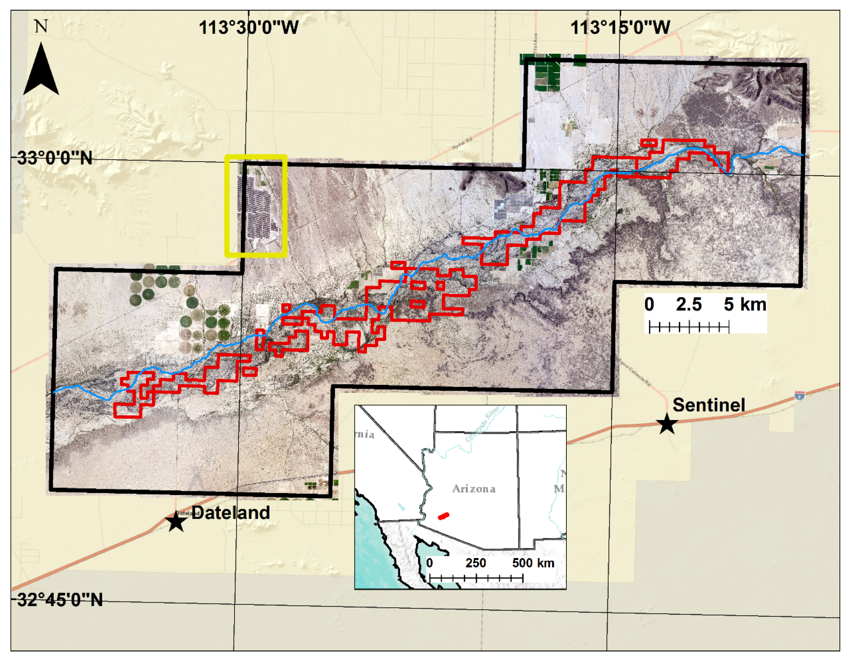
Our study area encompassed a nearly 42 km stretch of the Lower Gila River about 100 km northeast of Yuma, Arizona between Sentinel and Dateland, Arizona (Figure 1). The annual average temperature in the region is 23 degrees Celsius with annual average highs of 31 degrees Celsius and annual average lows of 14.5 degrees Celsius. Between 1994 and 2019, the average low has increased by about 2.25 degrees Celsius. The range between the minimum and maximum temperatures has decreased by about three degrees Celsius.
Average annual precipitation is just under 107 mm following a bimodal pattern with the majority of rainfall in the winter and summer months. Year-to-year precipitation is highly variable with a low of 15 mm in 1996 and a high of 166 mm in 2018. There has not been any clear decline in precipitation levels in the region over the last 25 years. Streamflow is minimal in the study area. Between 1994 and 2019, the U.S. Geological Survey (USGS) recorded less than 0.03 m3 per second of annual discharge 21 times (https://waterdata.usgs.gov/nwis).
Elevation at the northeastern side of the study area is 184 m above mean sea level sloping down to 110 m at the southwest side of the study area. The majority of the region is composed of entisols because the area is essentially all flood plain or riverbed (https://websoilsurvey.sc.egov.usda.gov/).
The Lower Gila River is a riparian system altered over the years through water diversion for agricultural purposes, electricity, and drought, creating a prime ecosystem for salt cedar. In the 1700s, fishing was possible on this stretch of the river and in the mid-1800s; cottonwoods grew to 9 m tall [10]. A 1972 survey identified six communities: cattails (Typha), salt cedar and arrowweed (Tamarix-Pluchea), mesquite (Prosopis), seepweed and pickleweed (Suaeda-Allenrolfea), saltbush (Atriplex), and creosote bush and mesquite (Larrea-Prosopis) [10]. The 1972 survey also stated that salt cedar encompassed about 50% of the study area [10].
According to the Bureau of Land Management (BLM), the current ecosystem along the Lower Gila River is composed of native species including mesquite (Prosopis velutina), creosote bush (Larrea tridentate), brittlebush (Encelia farinose), and arrowweed (Pluchea sericea). Cottonwood (Populus fremontii) and desert willow (Chilopsis linearis) are present near perennial waters, but those are rare or disappearing. The invasive salt cedar (Tamarix chinensis) encompasses most of the study area.
2.2. Data Acquisition and Preprocessing
2.2.1. Aerial Multispectral Imagery
The National Aerial Photography Program (NAPP) captured 3.75 min color infrared digital ortho quarter quads over the study during June and September of 1996. The nominal spatial resolution of the NAPP data was 1 m in 1996.
The National Agriculture Imagery Program (NAIP) acquired four-band multispectral aerial image data over the state of Arizona during 2007 and 2019. In 2007, acquisition of image data over the study area occurred between 30 June and 1 July. In 2019, acquisition of image data over the study area occurred between 16 June and 22 June. The nominal spatial resolution of the NAIP data was 1 m in 2017 and 60 cm in 2019.
The BLM acquisitioned the collection of digital orthoimagery over the study area, around 59 km2. On 22 May 2016, the Atlantic Group, LLC captured four-band multispectral aerial orthoimages. The nominal spatial resolution of the BLM data was 15 cm.
We created NDVI images from the red and near-infrared bands of all datasets.
2.2.2. Light Detection and Ranging (LiDAR)
On March 25, 2016, the Atlantic Group, LLC collected LiDAR data over the study area. The LiDAR data have a nominal pulse density of 16 pulses per m2 with a nominal pulse spacing of 0.2 m.
The Atlantic Group, LLC provided a LiDAR point cloud containing all returns along with one representing only bare earth data. Using FUSION [30], we created a Digital Elevation Model (DEM) raster with a spatial resolution of 50 cm based on the mean value of ground returns in each 50 cm cell. This was the finest resolution we could achieve without creating a surface with missing data due to a lack of returns in a cell.
We subtracted the bare earth DEM from the first return point cloud to create an Object Height Model (OHM). The OHM provided the normalized height of objects, including trees, above the ground. This allows the user to compare trees at different elevations as the subtraction normalizes for elevation.
We used the DensityMetrics tool in FUSION to compute point cloud densities at various height ranges. The DensityMetrics tool outputs a raster for each height interval dictated by the user wherein each pixel contains the proportion of LiDAR returns within that interval [30]. We calculated the densities of the point cloud within 50 cm cells at 1 m intervals, 0–1 m, 1–2 m, 2–3 m, 3–4 m, 4–5 m, and 5–6 m, for a total of six density measurements. There were no trees in the study area with a height greater than 6 m.
We used the IntensityImage tool in Fusion to convert the point cloud intensities to grid form. LIDAR intensity raster records the return strength of each LiDAR pulse in relation to the strength of the LiDAR pulse when the sensor emits it [30]. We calculated the average intensity within 50 cm cells.
We used the GridMetrics tool in Fusion to compute kurtosis and skewness from the original LiDAR point cloud and output the metrics as rasters with 50 cm cells. Both kurtosis and skewness characterize the distribution of LiDAR returns for each canopy in the study area. Skewness summarizes the asymmetry of points within each canopy, while kurtosis indicates how “peaky” the point distribution is in each canopy [30]. We selected kurtosis and skewness because of the compactness of mesquites compared to the more ambiguously shaped salt cedar.
2.2.3. Drone and Field Data
We collected drone imagery and ground-based photographs on 30 September 2016, 10 April 2017, 9 February 2018, and 8 May 2018 to identify vegetation species to train and validate our aerial imagery classification products. We collected the data in different seasons hoping to capture phenological differences between species. Our ground-based training methods started out as technicians walking through the study area on foot and geolocating class training data (tamarix, mesquite, other) using a GPS-enabled, hand-held camera or an iPad loaded with Galileo Offline Maps. We subsequently discovered that we could collect far more training data over a larger area with UAV imagery.
We flew a Phantom 3 Quadcopter and a Phantom 4 Pro Quadcopter 60 m above ground level within portions of the study area. The quadcopters carried a 12- and 20-megapixel camera, respectively, that captured standard red, green, blue color photographs. We surveyed eight ground control targets per acquisition with a hand-held Trimble GPS unit in order to produce orthomosaics in the same coordinate system as the 15 cm manned imagery. In total, we surveyed just under 20 hectares of the study area using the UAVs.
We stitched together ~1000 photos from each of the four drone flights using Agisoft Photoscan to create four high-resolution orthomosaics with ground sampling distances (pixel size) of 1.7 cm. The imagery was at a high enough resolution to visually identify and distinguish vegetation species including salt cedar, mesquite, and creosote.
2.2.4. Groundwater, Streamflow, Precipitation, and Water Equivalent Thickness Measurements
We acquired groundwater data from the Arizona Department of Water Resources (ADWR—https://waterdata.usgs.gov/nwis). We identified 15 different wells with measurements from 1994 through 2019. We calculated the percent change in depth to water for the 25-year period.
We also acquired streamflow data for the Gila River from a set of USGS (https://waterdata.usgs.gov/nwis) gauges located near Dateland (09520280) and Painted Rock Dam (09519800). The records include data from 1994 through 2020.
We used Parameter-Elevation Regressions on Independent Slopes Model (PRISM—https://prism.oregonstate.edu/) data to assess rainfall in the study area. PRISM data has a spatial resolution of 4 km. We extracted total monthly precipitation for the study area from 1994 through 2019. We calculated quarterly and yearly summations. We examined trends in precipitation and correlations between streamflow and precipitation.
We also examined water equivalent thickness measured by Gravity Recovery and Climate Experiment (GRACE) sensors [31,32,33]. GRACE measures the distance between twin satellites circling the earth to make gravitational field measurements. Collection of GRACE data began in 2002 and continues through to present day. Water equivalent thickness acts as a proxy for underground water storage provided as a three-degree equal-area grid.
2.3. Methodology
2.3.1. Classification of Vegetation in 2016 Using Acquired LiDAR and Multispectral Data
We used the C50 classification and regression tree (CART) R package to perform our classifications in this paper [34,35]. The C50 CART algorithm is a supervised machine learning technique that uses training data to create classification trees used to assign each pixel in a raster to a class. The tree outputs allow the user to assess confusion between classes and make adjustments to the training data to help distinguish classes.
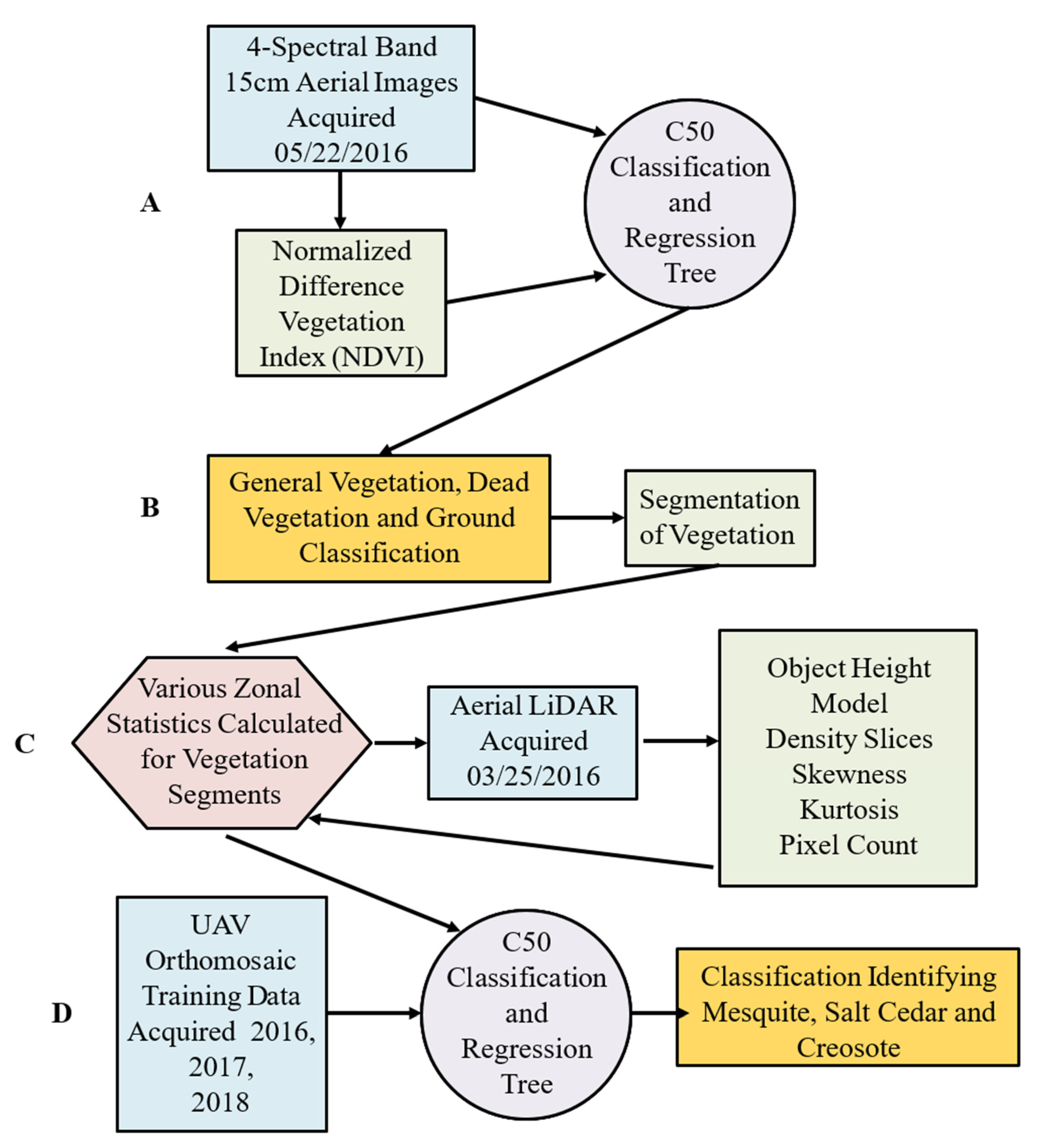
The spatial resolution, 15 cm, of the 2016 BLM image data was fine enough to produce a map of vegetation species in the study area. Our workflow to create a classified species map began with a C50 pixel-based classification into three general classes (detritus, vegetation, bare ground) (Figure 2A). We loaded the drone and field data into ArcGIS to select pixels representing detritus, vegetation, and bare ground on the BLM orthoimagery. Using ArcGIS, we created separate point shapefiles for each class containing 100 points representing 100 pixels. We performed the classification using the four-band orthoimagery and derived NDVI image. The classifier only needed one trial and winnowed three of the five inputs. It separated the three classes using information from the red band and NDVI layer. The classifier achieved an overall accuracy of 100 percent. The bright soil in the region made it easy to distinguish living vegetation and detritus.
We then merged the detritus and bare-ground classes to produce a vegetation and nonvegetation class. We used the region grouping tool, on pixels classified as vegetation, to combine adjacent pixels into segments (sometimes called objects). Each segment represents essentially one plant (except when canopies of multiple plants touched) (Figure 2B).
2.3.2. Vegetation Segment Metrics
We used zonal statistics in ArcMap to calculate several statistical measures for each vegetation segment (Figure 2C). We calculated the mean, maximum, minimum, range, and standard deviation of each band of the orthoimagery and the NDVI layer. We also calculated the mean, maximum, minimum, range, and standard deviation of the LiDAR height, skewness, kurtosis, and intensity information for each segment. Using the LiDAR density slices, we calculated the percentage of LiDAR returns in each segment for each of the six height levels. Finally, we counted the total number of 15 cm pixels within each vegetation segment. We used the various metrics in hopes of capturing the variance within each vegetation segment that would allow us to separate species (Table 1).
2.3.3. Classification of Vegetation Species
Using imagery collected via drone and GPS camera, we selected 258 segments representing individual salt cedars, 6 individual mesquites, and 24 individual creosotes. The amount of segments selected to represent each class varied because of the abundance of each species present in the study area. We could not accurately identify arrowweed and brittlebush on the 15 cm resolution orthophotos. However, it might be possible to pinpoint them on the higher resolution unmanned aerial vehicle (UAV) image data.
We partitioned the data in R, taking 50 percent of each class’ samples for training and setting aside 50 percent of each class’ samples for validation. We ran the C50 classifier on the various metrics in Table 1 with a maximum of 10 iterations. We also enabled boosting and winnowing of attributes.
2.3.4. Classification of Vegetation in 1996, 2007, and 2019 Using NAPP and NAIP Data
The spatial resolutions of the 1996, 2007, and 2019 data were not detailed enough to separate vegetation species from one another. However, we could identify areas of live vegetation, detritus, and bare ground.
Using the C50 package in R, we performed supervised classifications of pixels representing vegetation, detritus, and bare ground. We used the same protocol to train the C50 models for the 1996, 2007, and 2019 imagery sets. For training data, we selected 100 pixels, unique to each year, to represent the three classes. For validation purposes, we selected an additional 100 pixels per class, also unique to each year. We selected training samples using ESRI ArcMap 10.8 with Google Earth imagery as a reference. Class and image values (blue, green, red, NIR, NDVI) from each pixel were stored in point shapefiles.
C50 assesses the modeled output using both the training and validation pixels. Each classification achieved an overall accuracy of 100% when assessed with both sets of pixels. We manually delineated areas of active agricultural land in each of the three images.
2.3.5. Change Assessment
We created a tessellation, composed of 250 m squares (62,500 m2), using ArcGIS. We then used the Zonal Statistics tool to calculate the total number of vegetation pixels in each 250 m square from the 1996, 2007, and 2019 data. Using the Raster Calculator tool in ArcGIS, we calculated the percentage of vegetation in each square for each year. We subtracted the three tessellations to identify areas of increased vegetation and areas of decreased vegetation between each year and over the entire study period. We used the 250 m tessellation in hopes of identifying hotspots of vegetation loss and expansion.
2.3.6. Buffer Analysis
We obtained a shapefile representing the Gila River from the USGS National Hydrography Dataset. We created four concentric rings around the shapefile at 0–100 m, 100 m–500 m, 500 m–1000 m, and 1000 m–2000 m to examine vegetation in relation to the central river channel.
3. Results
3.1. Living Vegetation Segmentation Classification
The classification of the high-resolution aerial imagery and LiDAR from 2016 achieved an overall accuracy of 94 percent (Table 2). The C50 algorithm needed 13 out of 52 variables to separate the four different vegetation classes. The mining procedure used minimum, maximum, mean, and range of the blue band, mean of the green band, maximum, range, and standard deviation of the near infrared band, maximum and mean of the NDVI layer, density of LiDAR returns between 0 and 1 m, maximum of the OHM, and minimum skewness of the LiDAR returns.
The product exhibited confusion within all three classes. The classification process confused some of the larger creosote bushes for salt cedars. The algorithm also confused some of the small salt cedars for larger creosote bushes. The C50 algorithm correctly identified two of the three mesquite segments. The classification process misidentified only four of the segments representing salt cedars. It confused two with creosote and two with mesquite. The algorithm, in general, did an excellent job with the salt cedar class (Figure 3). Based on the classification, about 67 percent of BLM land in our study area is composed of bare ground. Detritus covers around 13 percent of the area and living vegetation covers the remaining 20 percent. Salt cedar makes up about 94 percent of the living vegetation. Mesquite and creosote make up equal amounts of the remaining 6 percent.
3.2. Vegetation Change and River Buffer Analysis
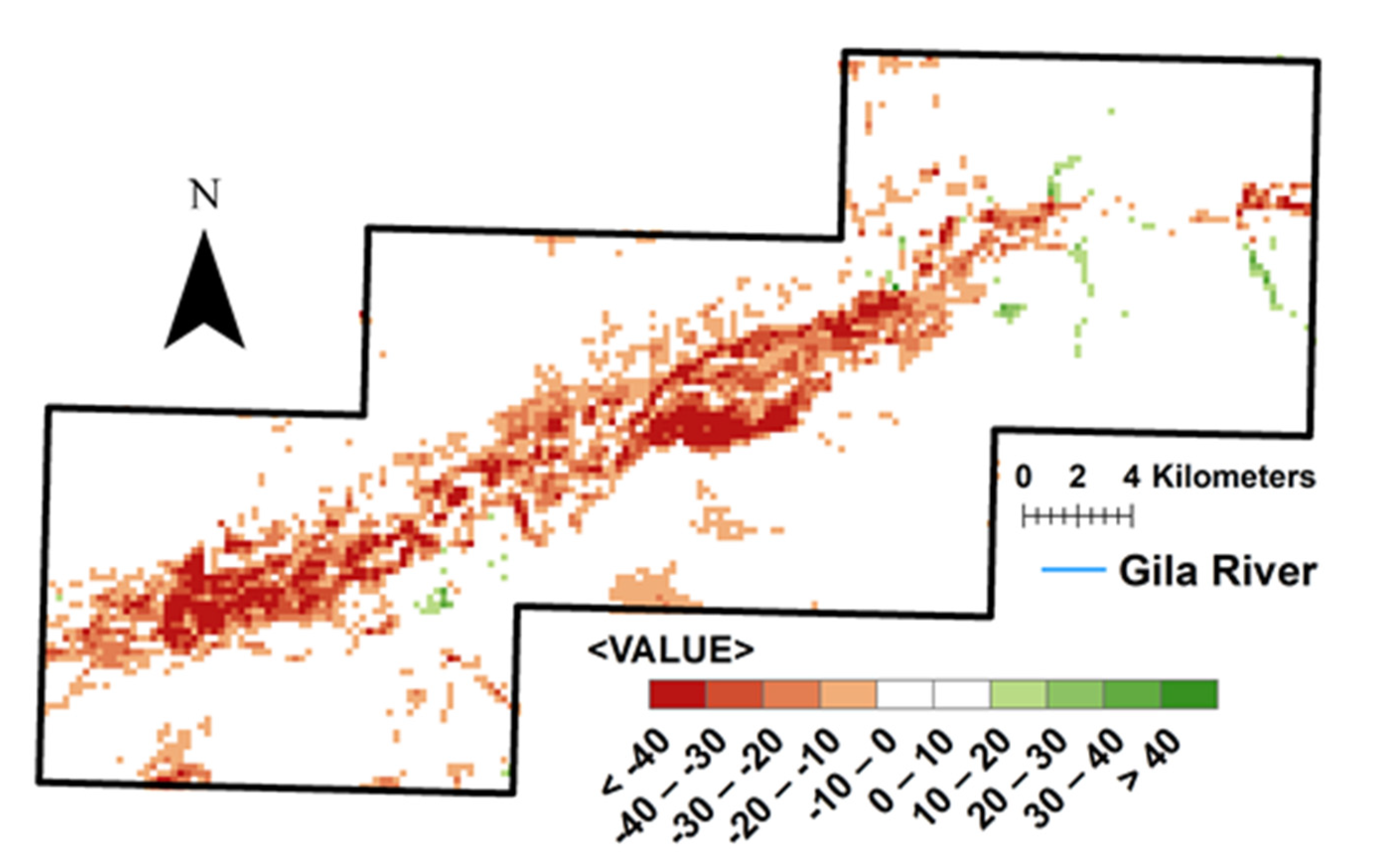
Based on the results of the classification processes, vegetation covered about 10 percent of the study area in 1996 (Figure A1), about 7 percent in 2007 (Figure A2), and around 4 percent in 2019 (Figure A3). This equates to around a 6 percent net decrease in vegetation over the entire study area during the last 23 years. There are certain portions of the study area showing pockets of increased vegetation, but most of the area has seen a decrease in vegetation (Figure 4). It seems most gains in vegetation are evident along stream channels. We used the buffer analysis to assess this phenomenon.
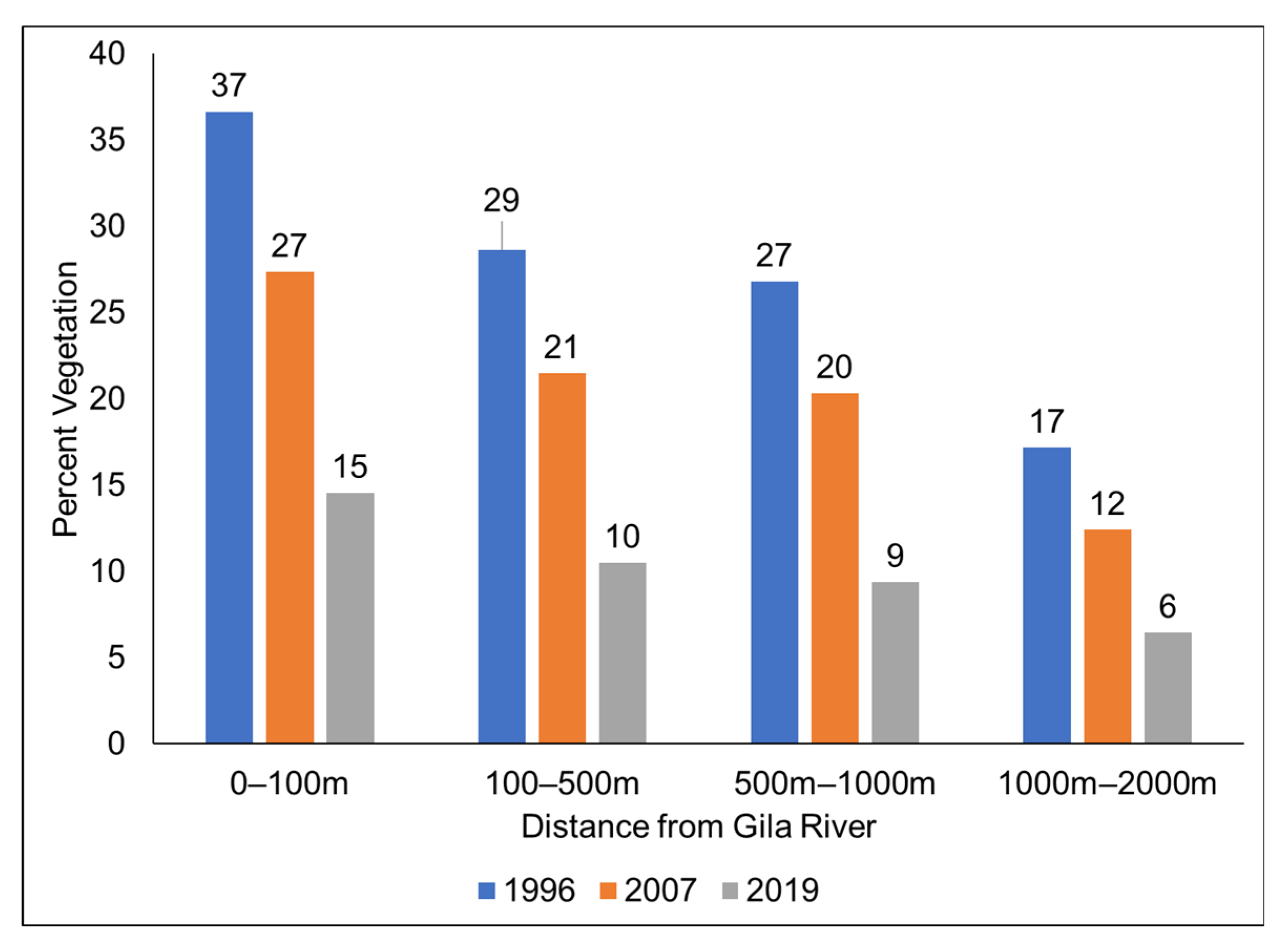
Based on the buffer analysis, the amount of vegetation was always greatest near the river and declined moving outward (Figure 5). The 0–100 m buffer also registered the greatest amount of vegetation loss, declining from 37% in 1996 to 15% in 2019. All four buffer levels exhibited the greatest amount of vegetation coverage in 1996 and the least amount of vegetation coverage in 2019.
3.3. Analysis of Water Data
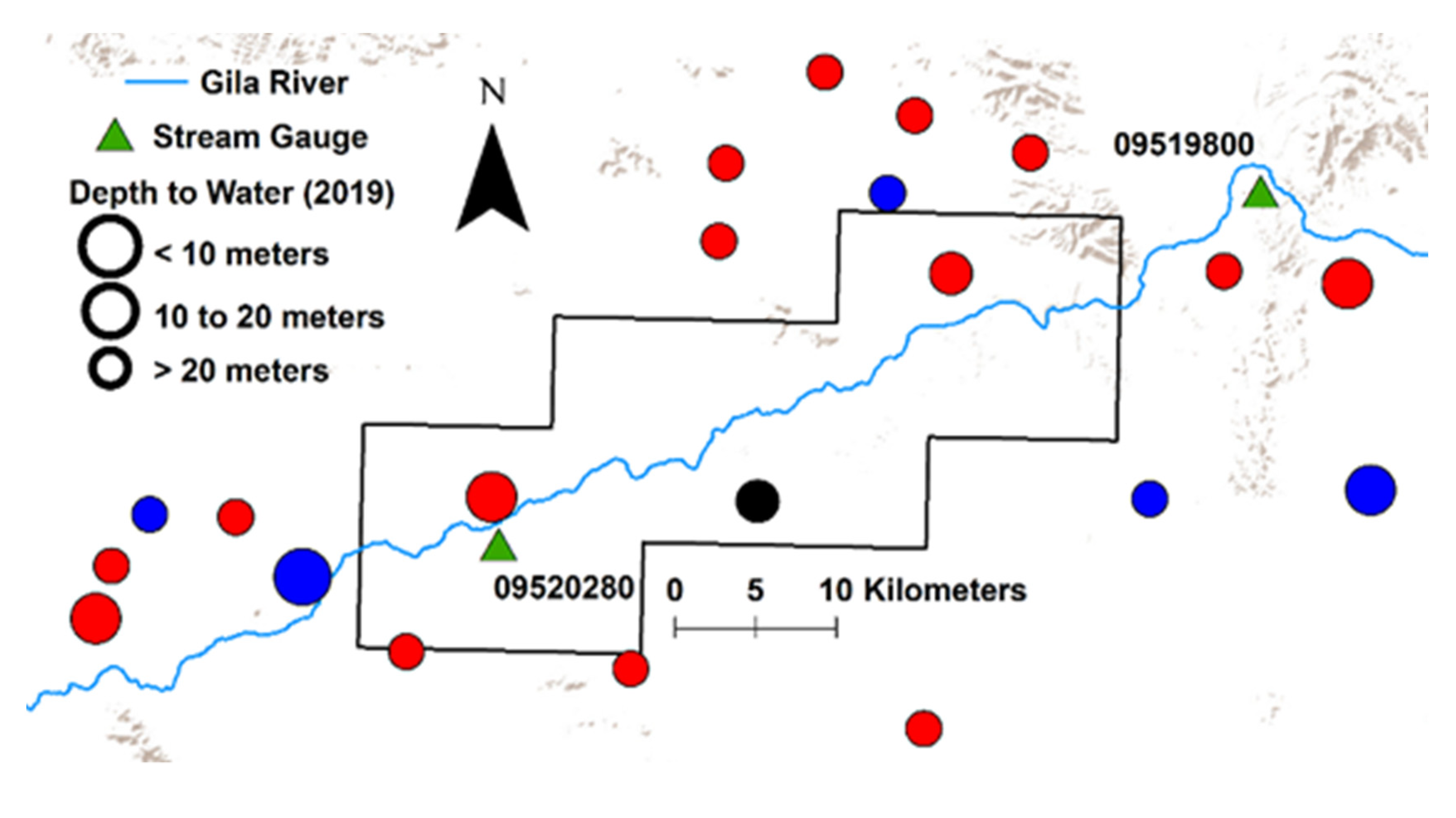
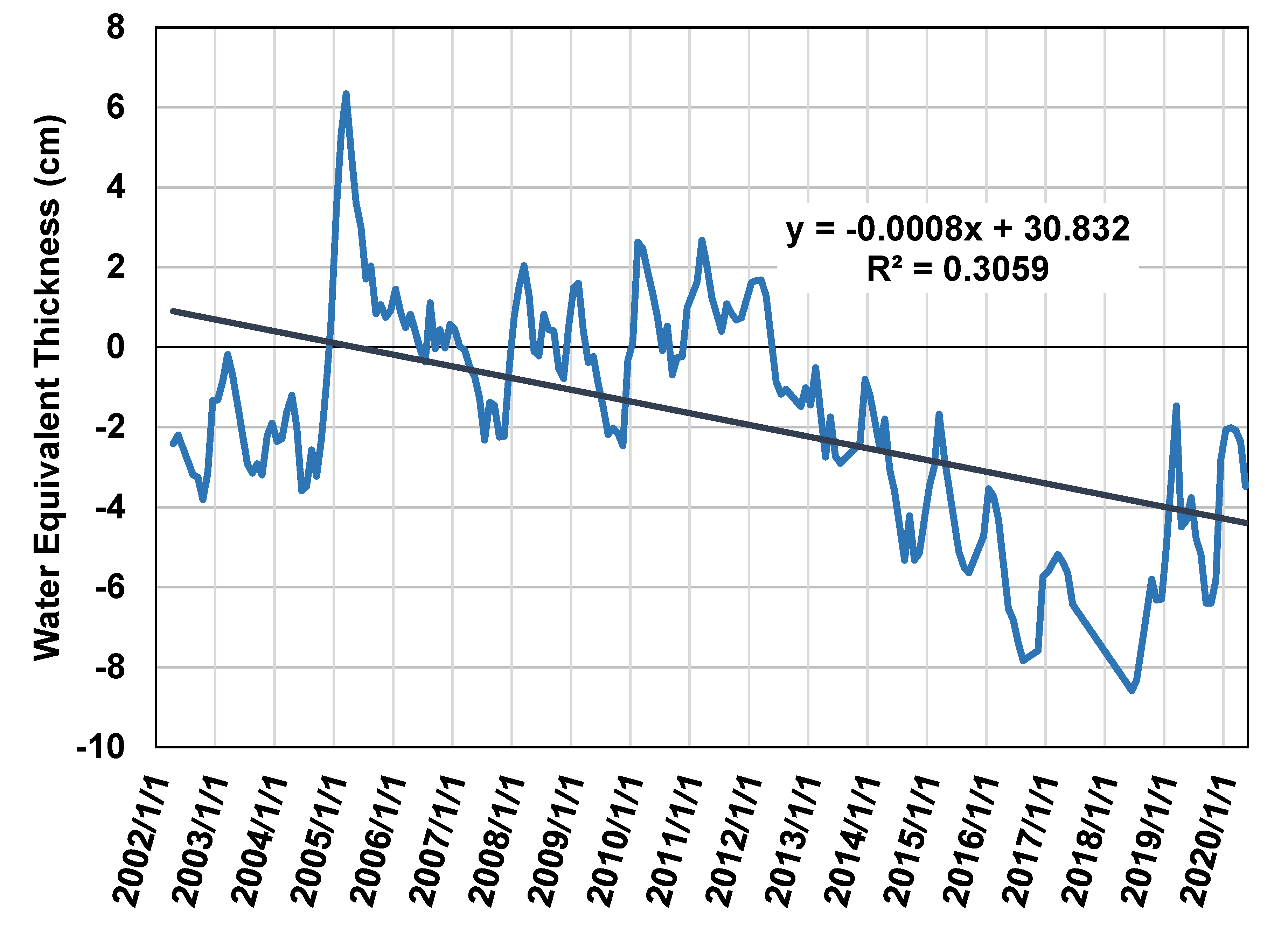
Fifteen of the twenty-one wells around the study area exhibit declining water levels (Figure 6). Based on the monthly water equivalent thickness measured by the GRACE, the amount of water in the region is declining (Figure 7).
Declining levels of water make it difficult for vegetation to remain established in the region. There is a clear decline in the amount of vegetation near the river channel and areas further from the river that already demonstrated low levels of vegetation show decline as well (Figure 5).
4. Discussion
4.1. Limitations and Improvements
For the 2016 species classification, we had a difficult time separating mesquite from salt cedar likely due to the limited point density of the LiDAR data, reducing our ability to characterize tree shape and height differences. The LiDAR used in this paper did not have a point density conducive to vegetation mapping in arid regions. We would need a LiDAR collection with a point density closer to 22 points per m2 in order to create LiDAR raster products with a pixel size near the 30 cm resolution of the multispectral data [36]. Ideally, to best separate tree species, multiple LiDAR returns, above, within, and below the canopy, would improve characterization of canopy structure.
UAV-based photogrammetric point clouds may aid vegetation classification in ways that LiDAR cannot. Specifically, those point clouds are typically much denser than LiDAR and may be able to better capture structural differences between vegetation species. Future work may include this technology with the recognition that UAVs can only cover small areas relative to the study area of this project. It may be relevant to use a UAV approach for prime conservation treatment and restoration area candidates.
Other work demonstrates the ability to separate tree species using hyperspectral data [37,38,39]. However, hyperspectral data are not readily available, are expensive to acquire, and require large storage capacity and powerful computing facilities. The user must employ advanced analysis techniques to reduce the data cube and extract the relevant information for species separation.
4.2. Vegetation and Water
It is clear from the species classification that salt cedar dominates our study area along the Lower Gila River. Based on a 1972 survey [10], researchers estimated that more than 50 percent of the plants in the floodplain were salt cedar. From the maps produced in our study, the amount of salt cedar in the study area has increased. Based on our 2016 classification, salt cedar now encompasses close to 90 percent of the living vegetation in our study region.
The 1972 survey also identified communities of Typha and Suaeda-Allenrolfea. Typha, commonly known as cattail, is reliant on standing or permanently running water. The stream gauge data for the study area indicates that stream flow is intermittent and minimal. Based on examination of the aerial photographs and our drone data, no standing water is present in the region. We did not encounter either of these communities on our many trips to the study area or identify them on the aerial photography and drone data. They may no longer be present in the study area, however, it would be difficult to identify either of these communities using our high-spatial-resolution aerial photographs or UAV data.
The change analysis showed that a majority of the study area lost vegetation cover between 1996 and 2019. We see the greatest loss in the 0–100 m buffer zone (Figure 5). We posed that agricultural activities were drawing water from the region. The amount of agriculture in the study area was low but doubled from 1 to 2 percent. Active agriculture made up one percent of the study area in 1996, increasing to two percent in 2007 and holding constant in 2019. However, the location of agricultural endeavors shifted. A solar facility replaced one of the larger sets of fields between 2007 and 2019 (Figure 1). A series of central pivot fields appeared between 1996 and 2007 and were still present in 2019.
Pumping of groundwater in the region may explain the vegetation loss in areas inside and outside of the stream channel. Groundwater well records indicate that the depth to water has increased throughout the area since 1994. We examined 21 wells around the study area and 15 of them show that the water table has declined between 1994 and 2019. Five of the wells surveyed are labeled for agricultural use and only one demonstrates an easier access to water (Figure 6).
Streamflow occasionally occurs in the region with extreme events happening intermittently. A large amount of water flowed along the Gila River in 1993/1994, 1995, 2005, and 2010 according to a USGS stream gauge (09520280) located on the river just north of Dateland. These flows only occur when water is released from the Painted Rock Dam upstream as the measurements from the surface water gauge (09519800) just below the dam have a 97 percent correlation with the measurements taken at the Dateland gauge. The Painted Rock Dam was built for flood control purposes with releases occurring due to storm events upstream [40].
Invasive salt cedar chokes stream flow further up the Gila River near Buckeye, Arizona. Community members are concerned about habitat degradation and increased wildfire risks [41]. A study conducted along the Pecos River in Texas discovered that removal of salt cedar along the river did not influence the stream flow. The authors state this is likely related to low sapwood area and the limited size of the salt cedar stands [42]. The situation on the Pecos River seems slightly different from the one along the Gila River as the salt cedar grows along the riverbank compared to in the main channel. Salt cedar is also present in the northern U.S. along the Musselshell River and Fort Peck Reservoir in Montana where scientists examined dispersal mechanisms [43].
There are no naturally occurring predators to salt cedar in North America to help limit the spread of the plant [43]. Managers have pursued various control methods over the years including cutting, burning, and removal to no avail [8,44]. Aerial spraying is a treatment option that seems to work, but requires years of reapplication costing millions of dollars [44,45]. In 2001, the United States Department of Agriculture (USDA) released the tamarisk beetle in California, Colorado, Utah, and Texas in an attempt to reduce the spread of salt cedar [44,46,47,48]. The beetles defoliate the salt cedar, disabling its ability to create seeds and weakening it to other elements. However, even successful management does not always mean that native species will return to dominance [11].
When the water does flow along the Gila River, it acts like a forest fire, clearing out dead detritus and allowing new vegetation to sprout. The extended length of the flows allows the water to infiltrate the soil and hydrate vegetation along the river.
5. Conclusions
We conducted this research to identify species along the Lower Gila River and determined salt cedar to be the dominant woody plant species. It is clear that the Lower Gila River is a prime environment for invasive salt cedar. The diversity of habitats documented in the 1970s has decreased. Species dependent on permanent water sources are no longer present in the region. Mesquite is present, but is having a hard time competing with salt cedar capable of drawing water from the surface and subterrain aquifers. Creosote, not dependent on water from the river, continues to be moderately present in the region.
We also examined changes in total vegetation cover over a 23-year period (1996 to 2019). The results show a decline of about 6 percent. The high accuracy of vegetation classifications indicates that vegetation loss is likely. While in the field, we observed numerous salt cedar skeletons, shown as detritus on the 2016 classification, to corroborate this conclusion. Locations of die-off may be an indication of water shortages in the region. If salt cedar can no longer survive along the Lower Gila River, few other plant species can.
The ability to measure vegetation conditions and species composition provides information about past and current ecosystem health. Once managers begin treatments along the Lower Gila River, we can use the techniques in this research to monitor and assess their impacts on the landscape. Creating a time series of maps will provide valuable information about the impact of restoration practices on the landscape.
A combination of environmental and human influences has led to a decline in biodiversity and a decline in healthy vegetation in general. The combination of damming upriver, groundwater withdrawal for agricultural purposes, and climate change has increased the chance of ecosystem collapse. Based on projections, the study area is expected to see an increase in overall temperatures, creating an even more arid environment [49]. If these trends continue, the amount of vegetation in the area will continue to decline and the amount of bare soil will continue to increase. This could lead to dust problems seen in other parts of the state and the world [50,51]. In the worst-case scenario, complete ecosystem transformation is possible.
Author Contributions
Conceptualization, W.J.v.L. and K.H.; methodology, W.J.v.L. and K.H; software, K.H. and J.K.G.; validation, K.H. and J.K.G.; formal analysis, K.H.; investigation, K.H.; resources, W.J.v.L.; data curation, K.H.; writing—original draft preparation, K.H.; writing—review and editing, K.H., J.K.G., and W.J.v.L.; visualization, K.H.; supervision, W.J.v.L.; project administration, W.J.v.L.; funding acquisition, K.H. and W.J.v.L. All authors have read and agreed to the published version of the manuscript.
Funding
This research was funded by the US Bureau of Land Management through cooperative agreement number L16AC00142.
Acknowledgments
The authors appreciate the research support provided by the Arizona Remote Sensing Center. We downloaded NAIP data from the USGS EarthExplorer website and GRACE data from the GRACE Data Analysis Tool. We are thankful to Jayanti Pokhrel and Charles Conley who helped with fieldwork.
Conflicts of Interest
The authors declare no conflict of interest. The funders had no role in the design of the study; in the collection, analyses, or interpretation of data; in the writing of the manuscript, or in the decision to publish the results.
Appendix A
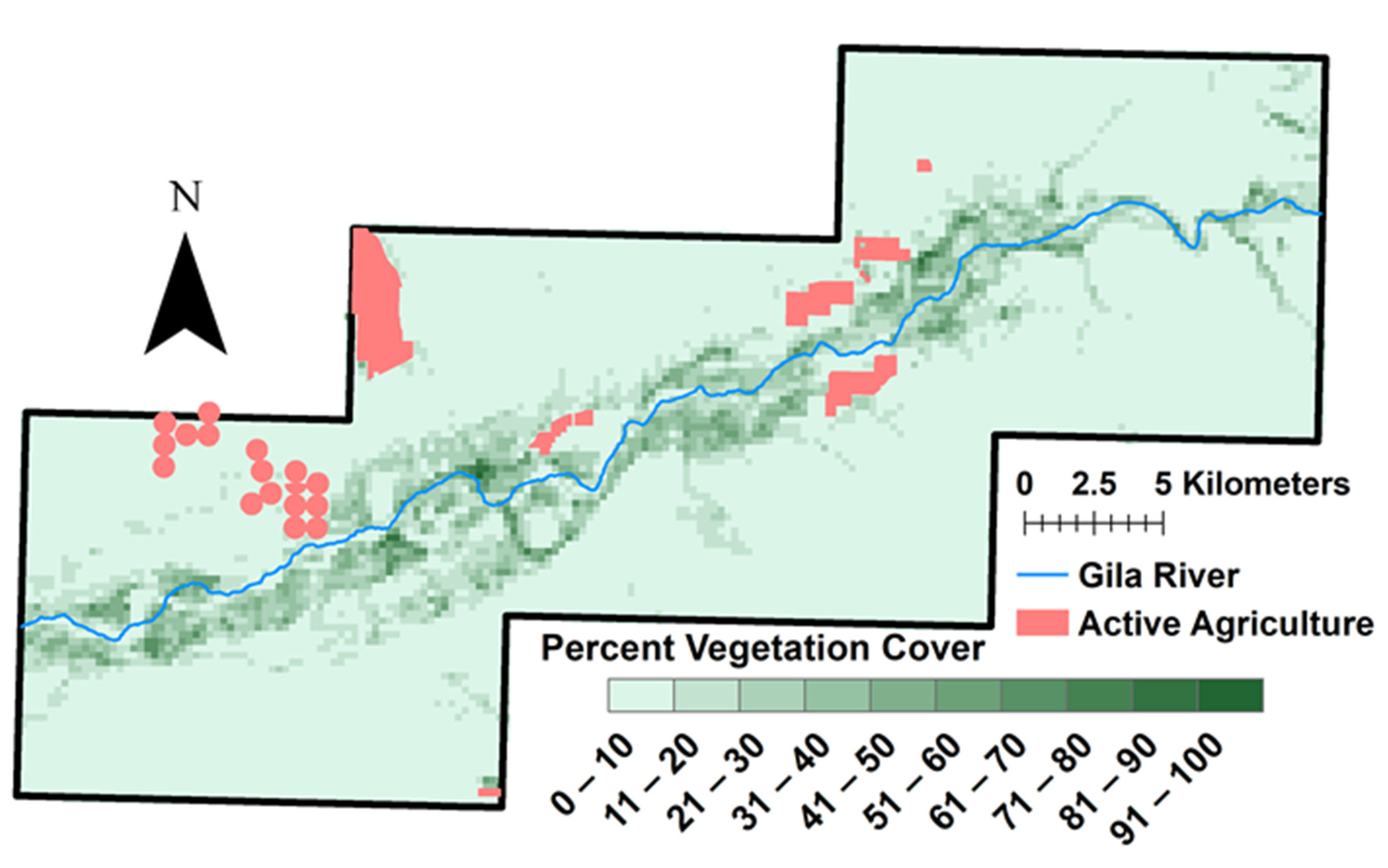
Figure A1.
Percent Vegetation Cover 1996. 250 m tessellation of vegetation cover in 1996. Areas with less cover are shown in light green and areas with greater cover are shown in dark green. Areas of active agriculture are shown in pink.
Figure A1.
Percent Vegetation Cover 1996. 250 m tessellation of vegetation cover in 1996. Areas with less cover are shown in light green and areas with greater cover are shown in dark green. Areas of active agriculture are shown in pink.

Figure A2.
Percent Vegetation Cover 2007. 250 m tessellation of vegetation cover in 2007. Areas with less cover are shown in light green and areas with greater cover are shown in dark green. Areas of active agriculture are shown in pink.
Figure A2.
Percent Vegetation Cover 2007. 250 m tessellation of vegetation cover in 2007. Areas with less cover are shown in light green and areas with greater cover are shown in dark green. Areas of active agriculture are shown in pink.

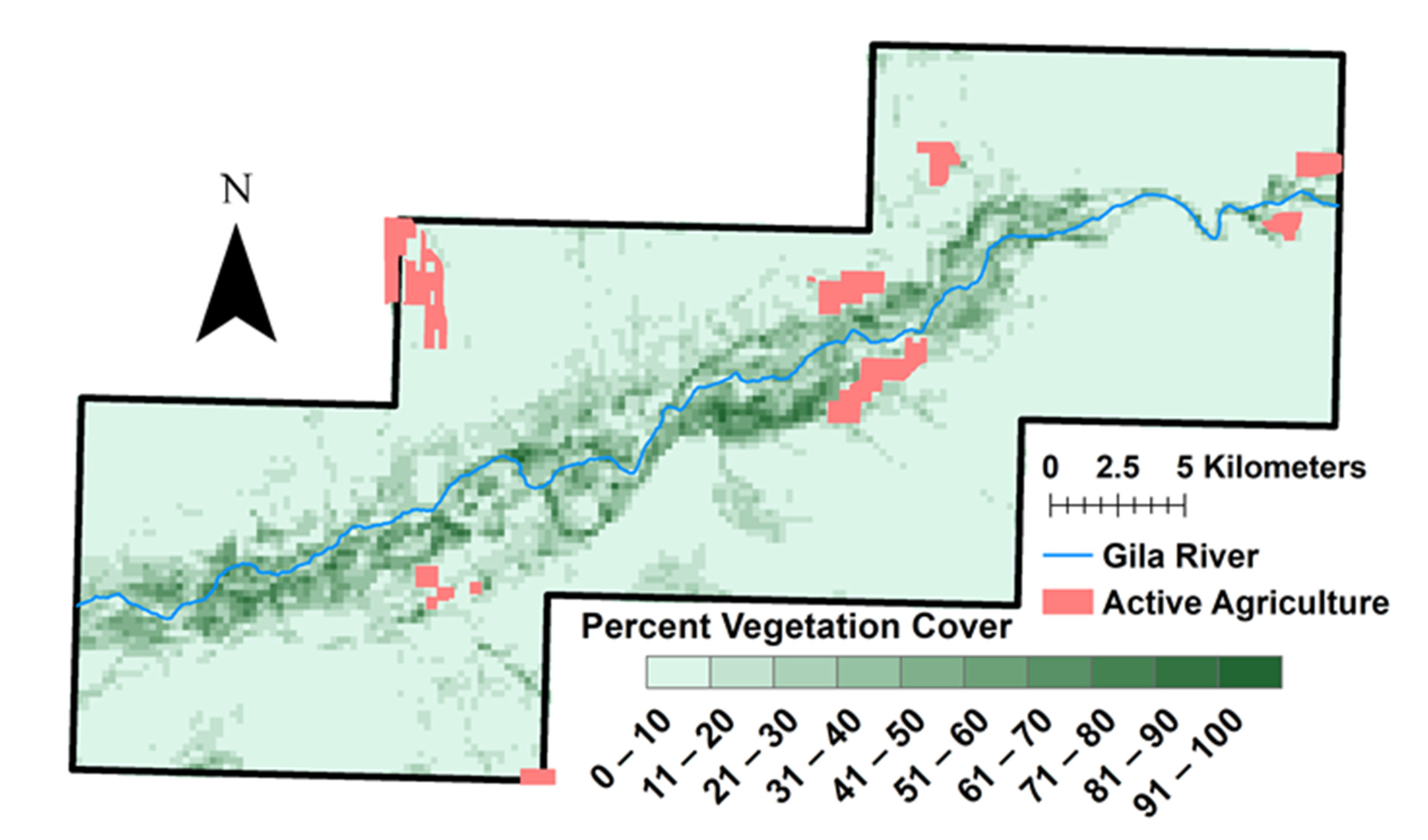
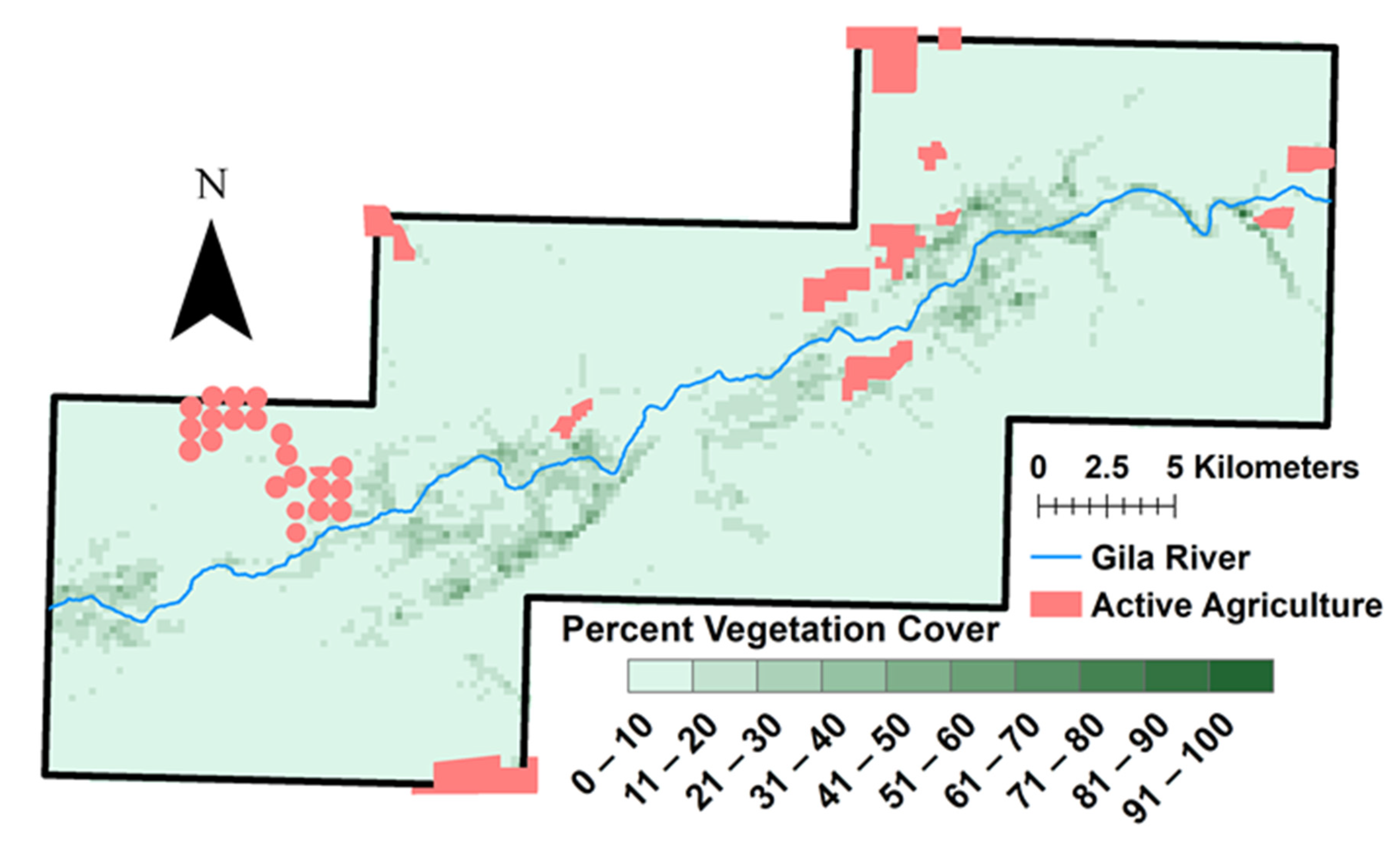
Figure A3.
Percent Vegetation Cover 2019. 250 m tessellation of vegetation cover in 2019. Areas with less cover are shown in light green and areas with greater cover are shown in dark green. Areas of active agriculture are shown in pink.
Figure A3.
Percent Vegetation Cover 2019. 250 m tessellation of vegetation cover in 2019. Areas with less cover are shown in light green and areas with greater cover are shown in dark green. Areas of active agriculture are shown in pink.

References
- Di Tomaso, J. Impact, biology, and ecology of saltcedar (tamarix spp.) in the southwestern united states. Weed Technol. 1998, 12, 326–336. [Google Scholar] [CrossRef]
- Bhattacharjee, J.; Taylor, J.; Smith, L.; Haukos, D. Seedling competition between native cottonwood and exotic saltcedar: Implications for restoration. Biol. Invasions 2009, 11, 1777–1787. [Google Scholar] [CrossRef] [Green Version]
- Stromberg, J. Functional equivalency of saltcedar (tamarix chinensis) and fremont cottonwood (populus fremonth) along a free-flowing river. Wetlands 1998, 18, 675–686. [Google Scholar] [CrossRef]
- Anderson, B.; Ohmart, R. Revegetation for Wildlife Enhancement along the Lower Colorado River; Arizona State University—Center for Environment Studies: Phoenix, AZ, USA, 1982. [Google Scholar]
- Anderson, B. Four Decades of Research on the Lower Colorado River; AVVAR Books: Blythe, CA, USA, 2011; p. 268. [Google Scholar]
- Sogge, M.; Paxton, E.; Tudor, A. Saltcedar and Southwestern Willow Flycatchers: Lessons from Long-Term Studies in Central Arizona; US Department of Agriculture, Forest Service, Rocky Mountain Research Station: Fort Collins, CO, USA, 2006.
- Stromberg, J.; Beauchamp, V.; Dixon, M.; Lite, S.; Paradzick, C. Importance of low-flow and high-flow characteristics to restoration of riparian vegetation along rivers in arid south-western united states. Freshw. Biol. 2007, 52, 651–679. [Google Scholar] [CrossRef]
- Chew, M. The monstering of tamarisk: How scientists made a plant into a problem. J. Hist. Biol. 2009, 42, 231–266. [Google Scholar] [CrossRef] [PubMed]
- Horton, J. The Development and Perpetuation of the Permanent Tamarisk Type in the Phreatophyte Zone of the Southwest; US Department of Agriculture, Forest Service, Rocky Mountain Forest and Range Experiment Station: Fort Collins, CO, USA, 1977.
- Haase, E. Survey of floodplain vegetation along the lower gila river in southwestern arizona. J. Ariz. Acad. Sci. 1972, 7, 75–81. [Google Scholar] [CrossRef]
- González, E.; Sher, A.; Anderson, R.; Bay, R.; Bean, D.; Bissonnete, G.; Cooper, D.; Dohrenwend, K.; Eichhorst, K.; El Waer, H.; et al. Secondary invasions of noxious weeds associated with control of invasive tamarix are frequent, idiosyncratic and persistent. Biol. Conserv. 2017, 213, 106–114. [Google Scholar] [CrossRef]
- Robinson, T. Introduction, Spread, and Areal Extent of Saltcedar (Tamarix) in the Western States; U.S. Government Printing Office: Washington, DC, USA, 1965.
- Nagler, P.; Glenn, E.; Jarnevich, C.; Shafroth, P. Distribution and abundance of saltcedar and russian olive in the western united states: Chapter 2. Saltcedar and Russian Olive Control Demonstration Act Science Assessment (Scientific Investigations Report 2009–5247); U.S. Geological Survey: Reston, VA, USA, 2010; pp. 11–31.
- Bedford, A.; Sankey, T.; Sankey, J.; Durning, L.; Ralston, B. Remote sensing of tamarisk beetle (diorhabda carinulata) impacts along 412 km of the colorado river in the grand canyon, arizona, USA. Ecol. Indic. 2018, 89, 365–375. [Google Scholar] [CrossRef]
- James, I.; O’Dell, R. Arizona’s Next Water Crisis Megafarms and Deeper Wells are Draining the Water Beneath Rural Arizona—Quietly, Irreversibly; The Arizona Republic: Phoenix, AZ, USA, 2019. [Google Scholar]
- Lahmers, T.; Eden, S. Water and Irrigated Agriculture in Arizona; University of Arizona Water Resources Research Center: Tucson, AZ, USA, 2018. [Google Scholar]
- Mendez-Estrella, R.; Romo-Leon, R.J.; Castellanos, E.A.; Gandarilla-Aizpuro, J.F.; Hartfield, K. Analyzing landscape trends on agriculture, introduced exotic grasslands and riparian ecosystems in arid regions of mexico. Remote Sens. 2016, 8, 664. [Google Scholar] [CrossRef] [Green Version]
- Romo-Leon, J.; van Leeuwen, W.; Castellanos-Villegas, A. Using remote sensing tools to assess land use transitions in unsustainable arid agro-ecosystems. J. Arid Environ. 2014, 106, 27–35. [Google Scholar] [CrossRef]
- Hultine, K.R.; Belnap, J.; van Riper, C.; Ehleringer, J.; Dennison, P.; Lee, M.; Nagler, P.; Snyder, K.; Uselman, S.; West, J. Tamarisk biocontrol in the western united states: Ecological and societal implications. Front. Ecol. Environ. 2010, 8, 467–474. [Google Scholar] [CrossRef] [Green Version]
- Taylor, J.; McDaniel, K. Restoration of saltcedar (tamarix sp.)-infested floodplains on the bosque del apache national wildlife refuge. Weed Technol. 1998, 12, 345–352. [Google Scholar] [CrossRef]
- McGwire, K.; Minor, T.; Fenstermaker, L. Hyperspectral mixture modeling for quantifying sparse vegetation cover in arid environments. Remote Sens. Environ. 2000, 72, 360–374. [Google Scholar] [CrossRef]
- Akasheh, O.; Neale, C.; Jayanthi, H. Detailed mapping of riparian vegetation in the middle rio grande river using high resolution multi-spectral airborne remote sensing. J. Arid Environ. 2008, 72, 1734–1744. [Google Scholar] [CrossRef]
- Walker, J.; Briggs, J. An object-oriented approach to urban forest mapping in phoenix. Photogramm. Eng. Remote Sens. 2007, 73, 577–583. [Google Scholar] [CrossRef]
- Ghamisi, P.; Rasti, B.; Yokoya, N.; Wang, Q.; Hofle, B.; Bruzzone, L.; Bovolo, F.; Chi, M.; Anders, K.; Gloaguen, R.; et al. Multisource and multitemporal data fusion in remote sensing: A comprehensive review of the state of the art. IEEE Geosci. Remote Sens. Mag. 2019, 7, 6–39. [Google Scholar] [CrossRef] [Green Version]
- Shen, X.; Cao, L. Tree-species classification in subtropical forests using airborne hyperspectral and lidar data. Remote Sens. 2017, 9, 1180. [Google Scholar] [CrossRef] [Green Version]
- Sankey, T.; Sankey, J.; Horne, R.; Bedford, A. Remote sensing of tamarisk biomass, insect herbivory, and defoliation: Novel methods in the grand canyon region, arizona. Photogramm. Eng. Remote Sens. 2016, 82, 645–652. [Google Scholar] [CrossRef]
- Sankey, J.; Munson, S.; Webb, R.; Wallace, C.; Duran, C. Remote sensing of sonoran desert vegetation structure and phenology with ground-based lidar. Remote Sens. 2015, 7, 342. [Google Scholar] [CrossRef] [Green Version]
- Ustin, S.; Gamon, J. Remote sensing of plant functional types. New Phytol. 2010, 186, 795–816. [Google Scholar] [CrossRef]
- John, R.; Chen, J.; Lu, N.; Guo, K.; Liang, C.; Wei, Y.; Noormets, A.; Ma, K.; Han, X. Predicting plant diversity based on remote sensing products in the semi-arid region of inner mongolia. Remote Sens. Environ. 2008, 112, 2018–2032. [Google Scholar] [CrossRef]
- McGaughey, R. Fusion/ldv Lidar Analysis and Visualization Software, 3.80; US Department of Agriculture, Forest Service, Pacific Northwest Research Station: Portland, OR, USA, 2018.
- Landerer, F.; Swenson, S. Accuracy of scaled grace terrestrial water storage estimates. Water Resour. Res. 2012, 48. [Google Scholar] [CrossRef]
- Swenson, S.; Wahr, J. Post-processing removal of correlated errors in grace data. Geophys. Res. Lett. 2006, 33. [Google Scholar] [CrossRef]
- Swenson, S. Grace Monthly Land Water Mass Grids Netcdf Release 5.0. Available online: http://dx.doi.org/10.5067/TELND-NC005 (accessed on 30 July 2020).
- Quinlan, J. C4.5 Programs for Machine Learning; Morgan Kaufmann Publishers: San Mateo, CA, USA, 1993. [Google Scholar]
- Kuhn, M. C5.0 Decision Trees and Rule-Based Models. Available online: https://cran.r-project.org/web/packages/C50/C50.pdf (accessed on 14 September 2020).
- Alonzo, M.; Bookhagen, B.; Roberts, D. Urban tree species mapping using hyperspectral and lidar data fusion. Remote Sens. Environ. 2014, 148, 70–83. [Google Scholar] [CrossRef]
- Maschler, J.; Atzberger, C.; Immitzer, M. Individual tree crown segmentation and classification of 13 tree species using airborne hyperspectral data. Remote Sens. 2018, 10, 1218. [Google Scholar] [CrossRef] [Green Version]
- Dalponte, M.; Bruzzone, L.; Gianelle, D. Fusion of Hyperspectral and Lidar Remote Sensing Data for Classification of Complex Forest Areas. IEEE Trans. Geosci. Remote Sens. 2008, 46, 1416–1427. [Google Scholar] [CrossRef] [Green Version]
- Asner, G.B.; Heidebrecht, K. Spectral Unmixing of Vegetation, Soil and Dry Carbon in Arid Regions: Comparing Multispectral and Hyperspectral Observations. Int. J. Remote Sens. 2002, 23, 3939–3958. [Google Scholar] [CrossRef]
- US Army Corps of Engineers. Operation of Alamo and Painted Rock Dams during Jan—Feb 1993 Floods; Reservoir Regulation Section: Los Angeles, CA, USA, 1993.
- Bowling, J. Progress is Made to Restore the Gila River’s Flow in Metro Phoenix after Decades of Planning; The Arizona Republic: Phoenix, AZ, USA, 2020. [Google Scholar]
- McDonald, A.K.; Wilcox, B.P.; Moore, G.W.; Hart, C.R.; Sheng, Z.; Owens, M.K. Tamarix transpiration along a semiarid river has negligible impact on water resources. Water Resour. Res. 2015, 51, 5117–5127. [Google Scholar] [CrossRef] [Green Version]
- Pearce, C.M.; Smith, D.G. Saltcedar: Distribution, abundance, and dispersal mechanisms, northern montana, USA. Wetlands 2003, 23, 215–228. [Google Scholar] [CrossRef]
- Larmer, P. Tackling Tamarisk; High County News: Paonia, CO, USA, 1998. [Google Scholar]
- Krza, P. It’s ‘Bombs Away’ on New Mexico Saltcedar; High County News: Paonia, CO, USA, 2003. [Google Scholar]
- Larmer, P. Fighting Exoctics with Exotics; High County News: Paonia, CO, USA, 1998. [Google Scholar]
- DeLoach, C.J.; Lewis, P.A.; Herr, J.C.; Carruthers, R.I.; Tracy, J.L.; Johnson, J. Host specificity of the leaf beetle, diorhabda elongata deserticola (coleoptera: Chrysomelidae) from asia, a biological control agent for saltcedars (tamarix: Tamaricaceae) in the western united states. Biol. Control 2003, 27, 117–147. [Google Scholar] [CrossRef] [Green Version]
- Mast, K. The beetle, the bird and the tamarisk tree. In Discover; Kalmbach Media CO: Waukesha, WI, USA, 2018. [Google Scholar]
- Gonzalez, P.; Garfin, G.; Breshears, D.; Brooks, K.; Brown, H.; Elias, E.; Gunasekara, A.; Huntly, N.; Maldonado, J.; Mantua, N.; et al. Southwest. In Impacts, Risks, and Adaptation in the United States: Fourth National Climate Assessment, Volume ii; U.S. Global Change Research Program: Washington, DC, USA, 2018; pp. 1101–1184. [Google Scholar]
- Zhang, A.; Zheng, C.; Wang, S.; Yao, Y. Analysis of streamflow variations in the heihe river basin, northwest china: Trends, abrupt changes, driving factors and ecological influences. J. Hydrol. Reg. Stud. 2015, 3, 106–124. [Google Scholar] [CrossRef] [Green Version]
- Wang, X.; Dong, Z.; Zhang, J.; Liu, L. Modern dust storms in china: An overview. J. Arid Environ. 2004, 58, 559–574. [Google Scholar] [CrossRef]
Figure 1.
Location of Study Area. Our study area, indicated in black on the inset map, is composed of a nearly 50 km stretch of the Gila River located between Sentinel, AZ (east) and Dateland, AZ (west). This 60 cm natural color National Agriculture Imagery Program (NAIP) image from 2019 shows private agricultural land use both north and south of the Gila River (blue line). The area outlined in yellow was converted from agriculture into a solar energy facility after 2010. Lands managed by the Bureau of Land Management (BLM) are outlined in red, which also delineates the extent of the light detection and ranging (LiDAR) collection used in this paper. Cities of interest are shown as black stars.

Figure 2.
Workflow Diagram. (A) We performed a classification using the high-resolution multispectral imagery to identify vegetation, detritus, and bare ground in the study area. (B) We created segments representing vegetation by grouping conjoining vegetation pixels. (C) We extracted metrics derived from the photographs and LIDAR data for each vegetation segment. (D) Using the C50 algorithm, we identified the species type of each segment.

Figure 3.
Results of 2016 classification. We used a classification and regression tree (CART) classification using a combination of high-spatial-resolution aerial imagery and LiDAR data from 2016. The algorithm created a highly accurate map of current plant species along the Lower Gila River on BLM lands. This figure highlights a tiny area within the study area showing detritus in light grey, bare ground in tan, creosote segments in purple, mesquite segments in light green, and the salt cedar segments in dark green.
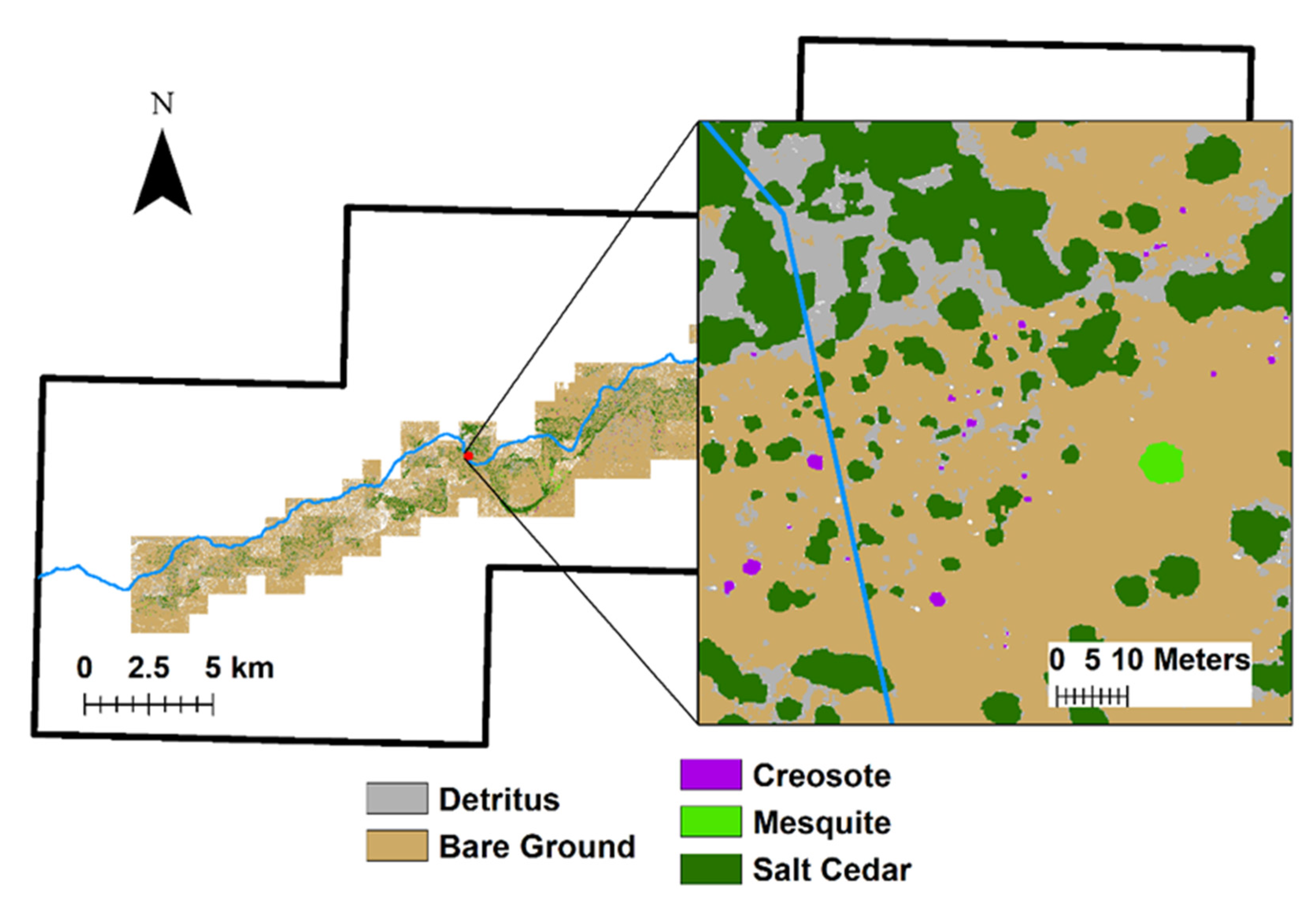
Figure 4.
Map of vegetation change from 1996 to 2019. We subtracted the 250 m tessellation of vegetation cover in 1996 from the 250 m tessellation of vegetation cover in 2019. Areas in red indicate loss of vegetation, darker shades indicate greater loss. Areas in green indicate increased vegetation with darker shades indicating greater increases. Even though a large amount of area appears red, keep in mind that all the area in white experienced little to no change. See appendix for percent vegetation cover maps from 1996, 2007, and 2019.

Figure 5.
Amount of vegetation in relation to distance from Gila River 1996, 2007 and 2019. We created buffers at 0–100 m, 100 m–500 m, 500 m–1000 m, and 1000 m–2000 m from the Gila River in our study area. We then calculated the percentage of vegetation cover in each buffer for 1996, 2007, and 2019 using the classified rasters.

Figure 6.
Location of wells and stream gauges in relation to the study area. There are 21 indexed wells, shown as circles, located in and around the study area. Larger circles represent wells with lower depth to water and smaller circles represent greater depth to water. Wells shown in red indicate wells where the depth to water has increased since 1992, while wells shown in blue indicate wells where the depth to water has decreased since 1992. The well displayed in black did not register a change in depth. USGS stream gauge locations are shown as green triangles. The Dateland gauge (09520280) is on the western side of the map and the Painted Dam gauge (09519800) is on the eastern side of the map. The study area shown in Figure 1 is represented by the black box.

Figure 7.
Change in water equivalent thickness 2002 to 2020. Gravity Recovery and Climate Experiment (GRACE) sensors provide monthly measurements of water equivalent thickness. This chart shows data for the pixel encompassing the area surrounding the study area. This information can be interpreted as a proxy for trends in ground water for our study area.


Table 1.
Metrics used to perform 2016 classification. We computed a variety of metrics from the orthoimagery and LiDAR data. Using zonal statistics, we derived various statistical measures for each vegetation segment in the study area.
Table 1.
Metrics used to perform 2016 classification. We computed a variety of metrics from the orthoimagery and LiDAR data. Using zonal statistics, we derived various statistical measures for each vegetation segment in the study area.
| Metric | Mean | Max | Min | Standard Deviation | Range | Sum |
|---|---|---|---|---|---|---|
| Blue Band | X | X | X | X | X | |
| Green Band | X | X | X | X | X | |
| Red Band | X | X | X | X | X | |
| NIR Band | X | X | X | X | X | |
| NDVI | X | X | X | X | X | |
| LiDAR Height | X | X | X | X | X | |
| LiDAR Intensity | X | X | X | X | X | |
| LiDAR Kurtosis | X | X | X | X | X | |
| LiDAR Density 0–1 m | X | |||||
| LiDAR Density 1–2 m | X | |||||
| LiDAR Density 2–3 m | X | |||||
| LiDAR Density 3–4 m | X | |||||
| LiDAR Density 4–5 m | X | |||||
| LiDAR Density 5–6 m | X | |||||
| LiDAR Skewness | X | X | X | X | X | |
| Pixel Count | X |
Table 2.
Error matrix for 2016 classification. The classification output achieved an overall accuracy of 94 percent. Confusion occurred among the various classes mainly attributed to the size of segments.
Table 2.
Error matrix for 2016 classification. The classification output achieved an overall accuracy of 94 percent. Confusion occurred among the various classes mainly attributed to the size of segments.
| Reference | ||||
|---|---|---|---|---|
| Creosote | Mesquite | Salt Cedar | ||
| Creosote | 8 | 0 | 2 | |
| Prediction | Mesquite | 0 | 2 | 2 |
| Salt Cedar | 4 | 1 | 125 | |
| Overall Accuracy: 94% Overall Kappa: 0.66 | ||||
© 2020 by the authors. Licensee MDPI, Basel, Switzerland. This article is an open access article distributed under the terms and conditions of the Creative Commons Attribution (CC BY) license (http://creativecommons.org/licenses/by/4.0/).
Share and Cite
MDPI and ACS Style
Hartfield, K.; Leeuwen, W.J.D.v.; Gillan, J.K. Remotely Sensed Changes in Vegetation Cover Distribution and Groundwater along the Lower Gila River. Land 2020, 9, 326. https://doi.org/10.3390/land9090326
AMA Style
Hartfield K, Leeuwen WJDv, Gillan JK. Remotely Sensed Changes in Vegetation Cover Distribution and Groundwater along the Lower Gila River. Land. 2020; 9(9):326. https://doi.org/10.3390/land9090326
Chicago/Turabian StyleHartfield, Kyle, Willem J.D. van Leeuwen, and Jeffrey K. Gillan. 2020. "Remotely Sensed Changes in Vegetation Cover Distribution and Groundwater along the Lower Gila River" Land 9, no. 9: 326. https://doi.org/10.3390/land9090326
Note that from the first issue of 2016, this journal uses article numbers instead of page numbers. See further details here.