Remotely-Sensed Surface Temperature and Vegetation Status for the Assessment of Decadal Change in the Irrigated Land Cover of North-Central Victoria, Australia


Abstract
:1. Introduction
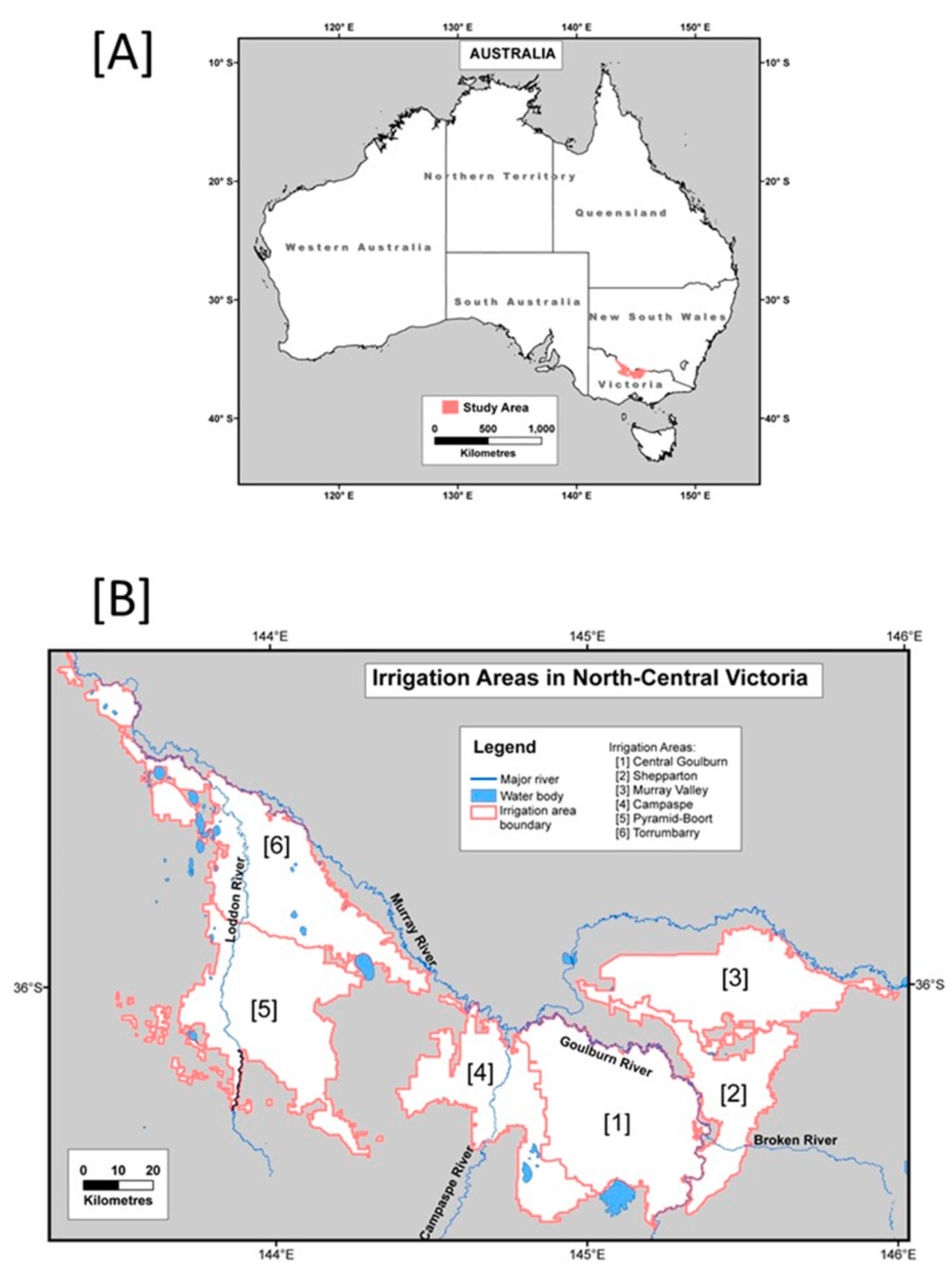
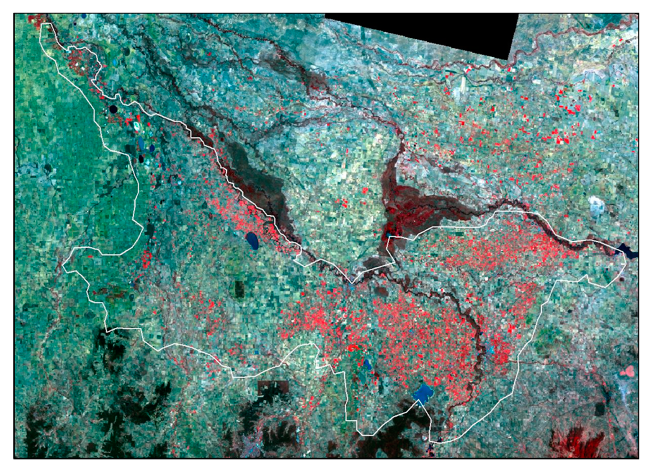
2. Study Area
3. Materials and Methods
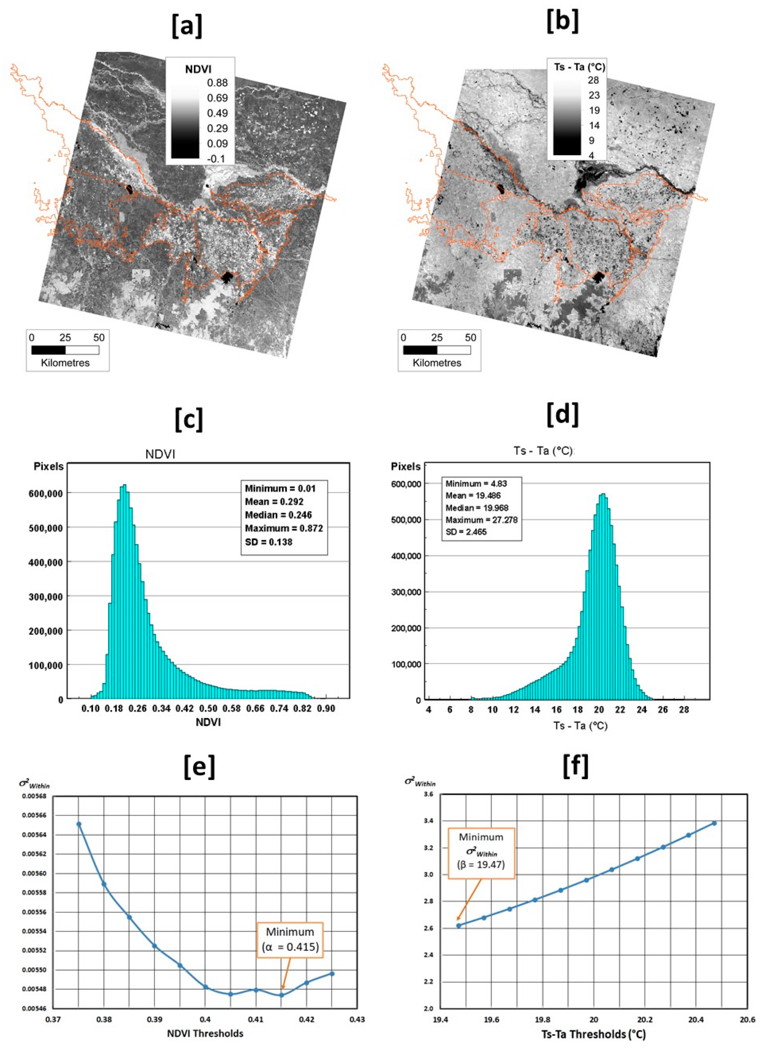
3.1. Step 1: Data Preparation
- = Planetary TOA reflectance [-]
- = Mathematical constant equal to ~3.14159 [-]
- = Spectral radiance [W/ (m2 sr μm)]
- = Earth-Sun distance [Astronomical units]
- = Mean exoatmospheric solar irradiance [W/(m2 μm)]
- = Solar zenith angle [Degrees].
- Ts = Effective at-sensor brightness temperature [K]
- K2 = Calibration constant 2 [K]
- K1 = Calibration constant 1 [W/ (m2 sr μm)]
- Lλ = Spectral radiance at the sensor’s aperture [W/ (m2 sr μm)]
- ln = Natural logarithm.
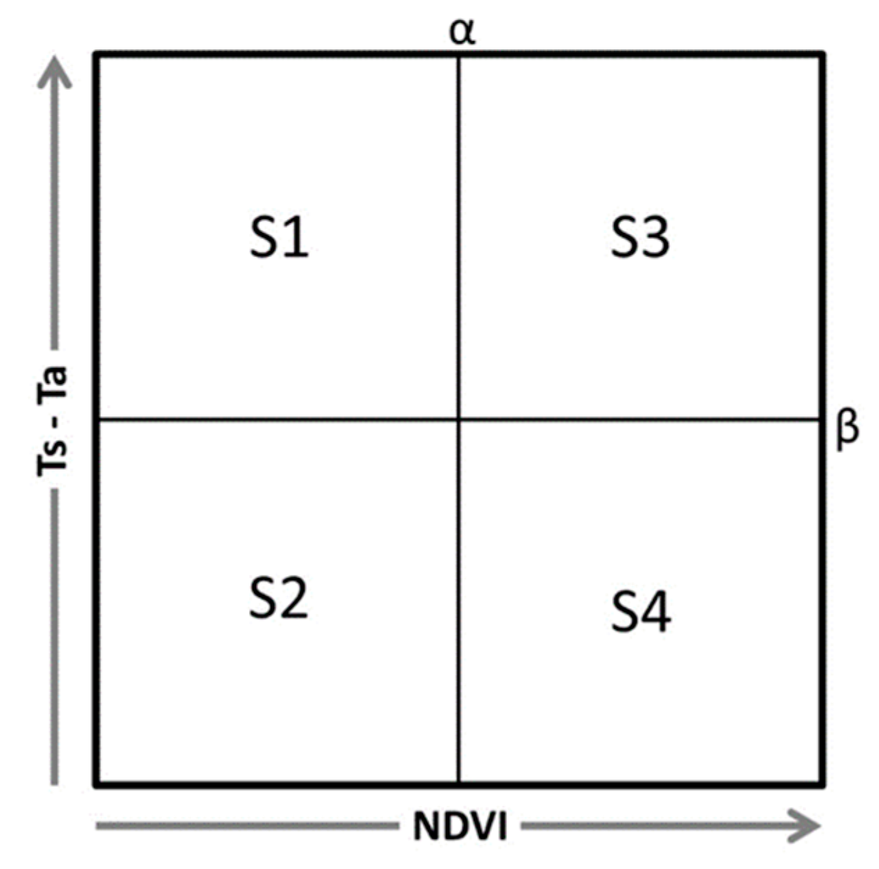
3.2. Step 2: Thresholding Process
3.3. Step 3: Identifying Irrigated Land Cover Classes
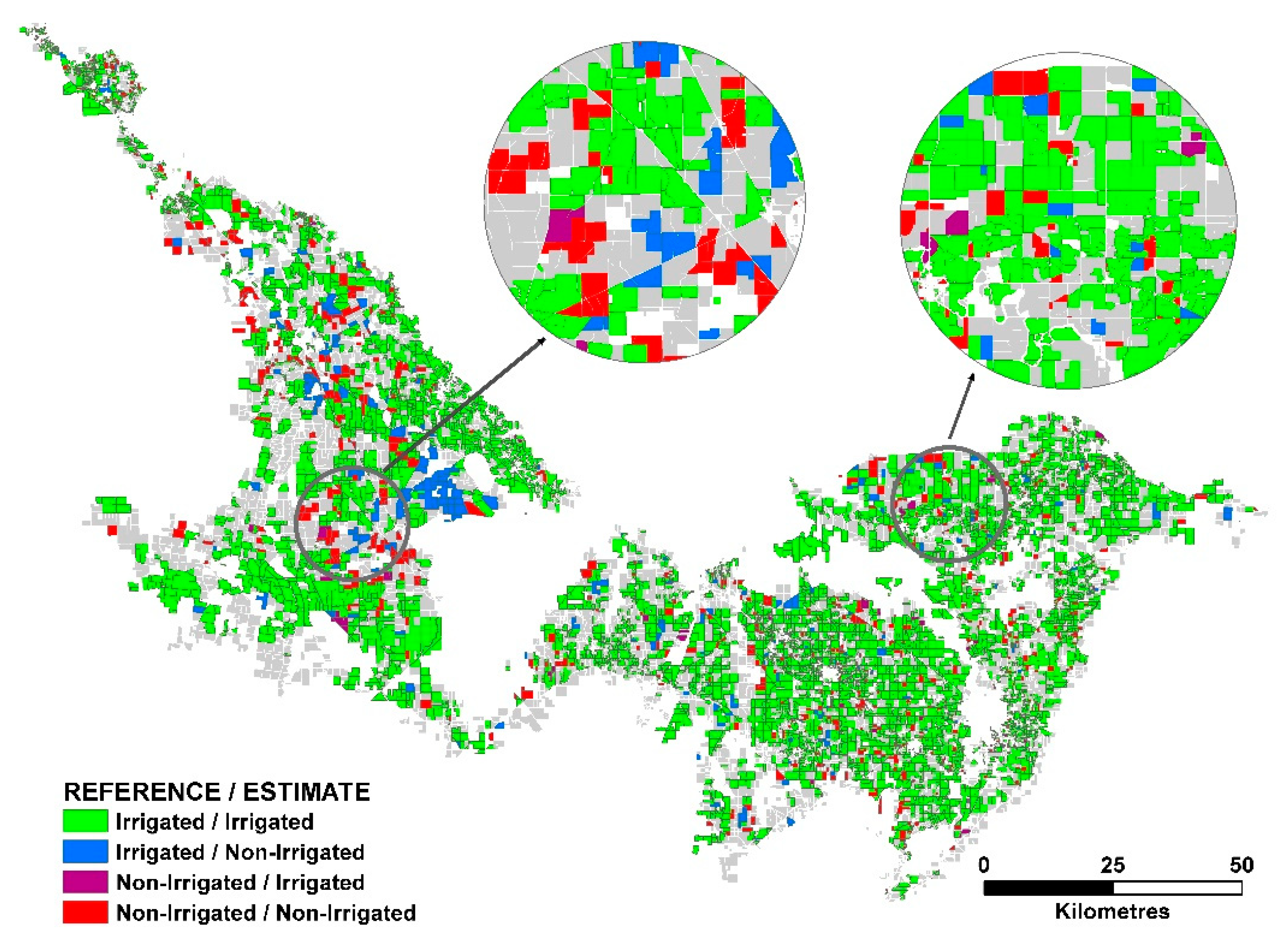
3.4. Step 4: Evaluating the Irrigated Land Cover Changes
4. Results
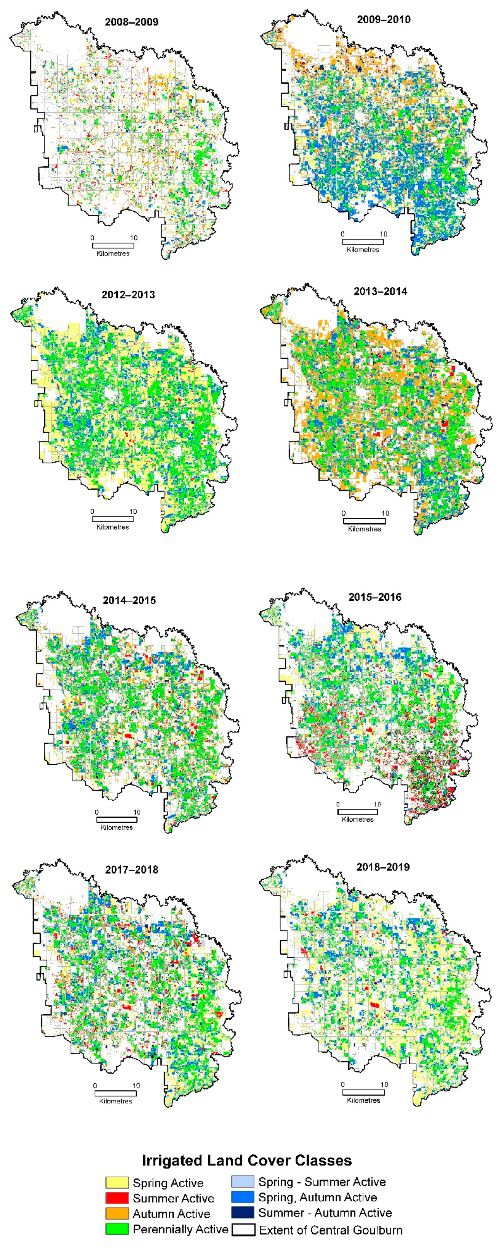
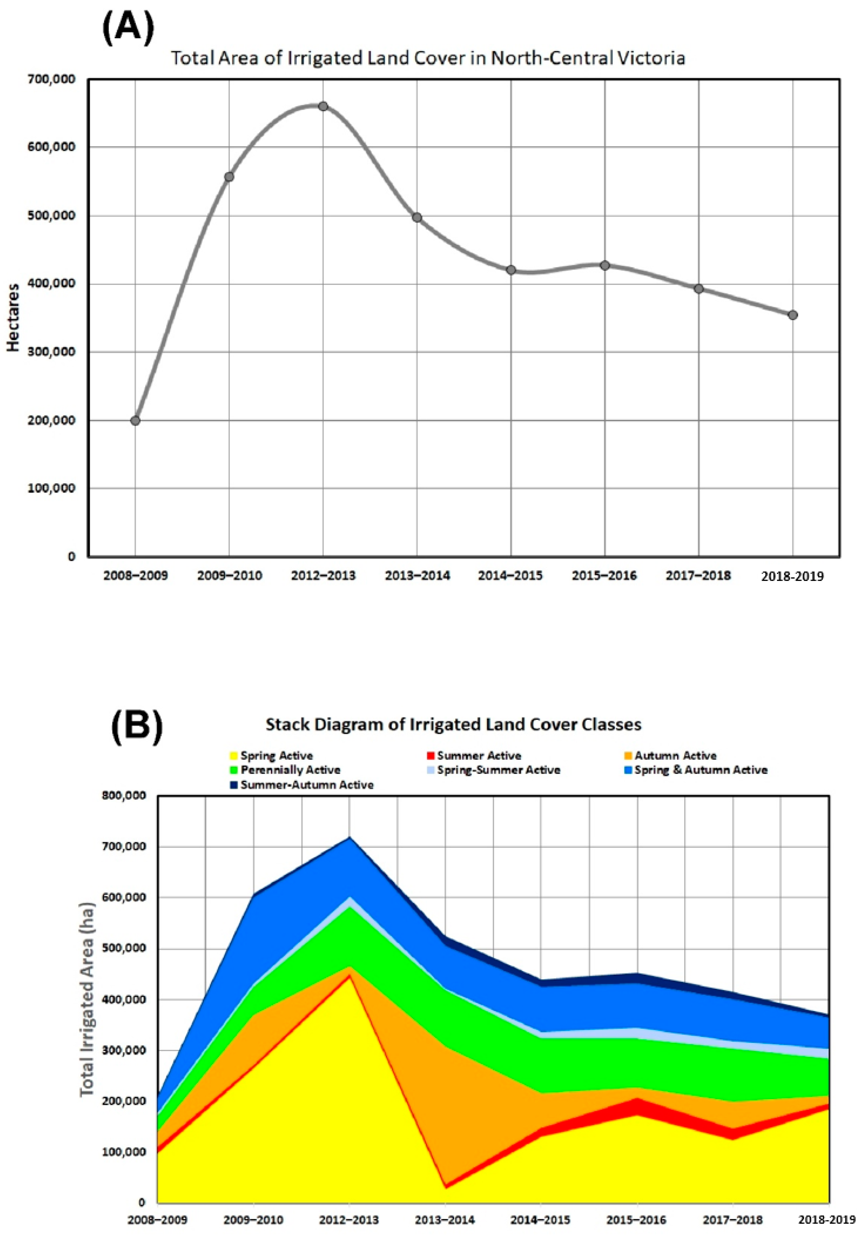
4.1. Regional Changes
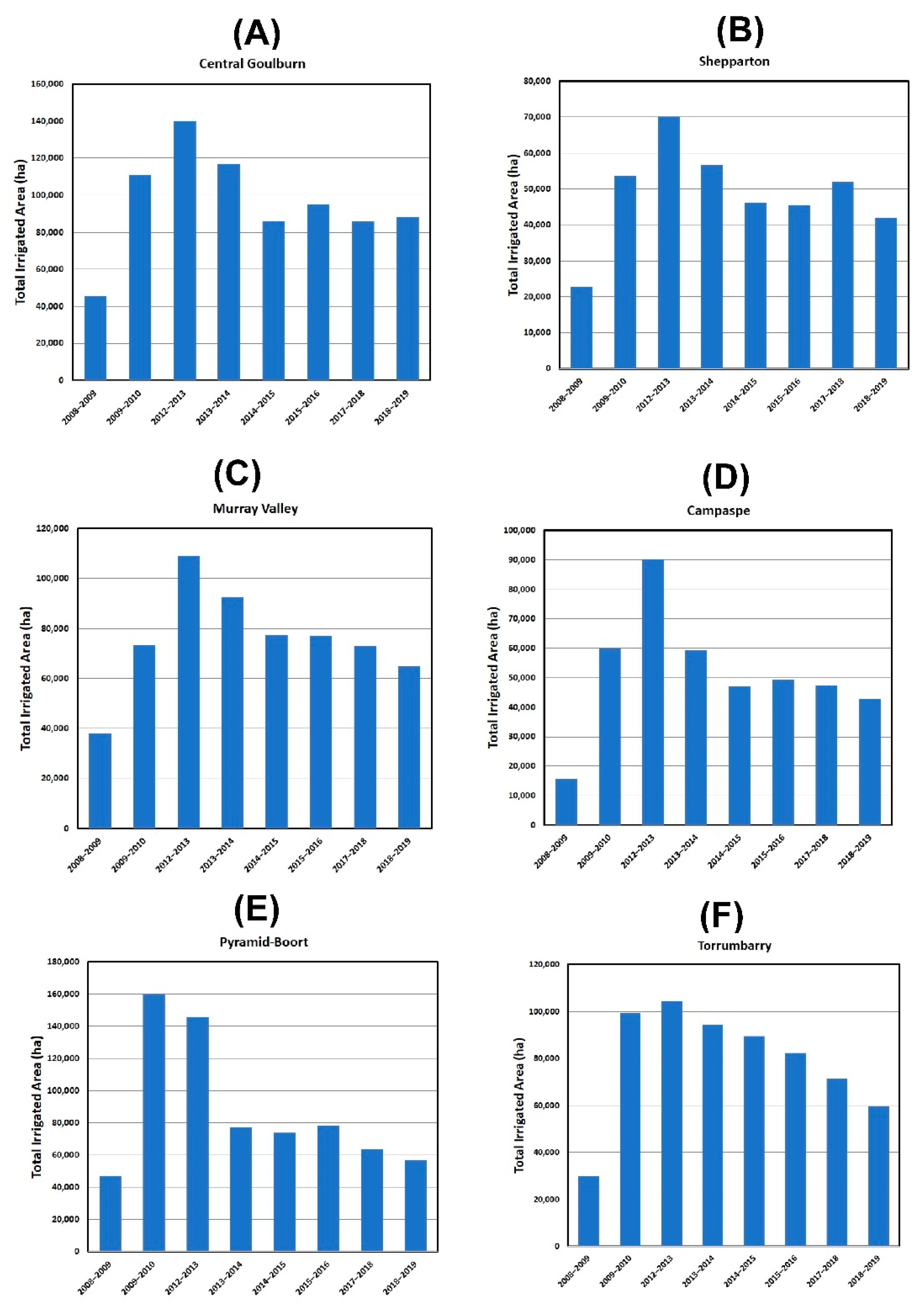
4.2. Changes in Sub-Regions
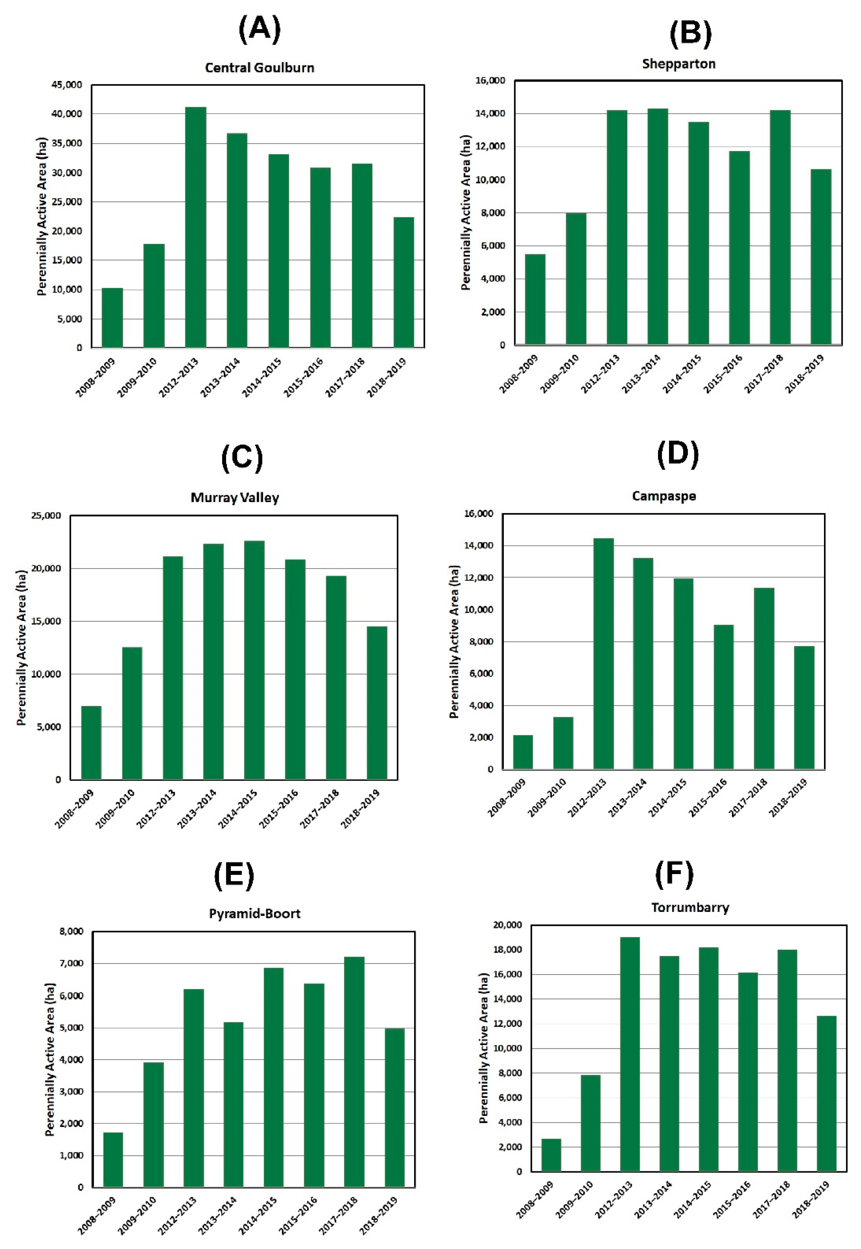
4.3. Changes in Perennially Active Class across Sub-Regions
5. Discussion
6. Conclusions
Author Contributions
Funding
Acknowledgments
Conflicts of Interest
References
- Colaizzi, P.; Bliesner, R.; Hardy, L. A Review of Evolving Critical Priorities for Irrigated Agriculture. In World Environmental and Water Resources Congress 2008; Raymond 1-15; Roger, W., Babcock, W., Jr., Eds.; American Society of Civil Engineers: Reston, VA, USA, 2008. [Google Scholar]
- World Bank. “Water in Agriculture.” World Bank. Available online: https://www.worldbank.org/en/topic/water-in-agriculture (accessed on 6 July 2020).
- Weiss, M.; Jacob, F.; Duveiller, G. Remote Sensing for Agricultural Applications: A Meta-Review. Remote Sens. Environ. 2020, 236, 111402. [Google Scholar] [CrossRef]
- Aleksandrova, M.; Lamers, J.P.; Martius, C.; Tischbein, B. Rural Vulnerability to Environmental Change in the Irrigated Lowlands of Central Asia and Options for Policy-Makers: A Review. Environ. Sci. Policy 2014, 41, 77–88. [Google Scholar] [CrossRef]
- Alvino, A.; Marino, S. Remote Sensing for Irrigation of Horticultural Crops. Horticulturae 2017, 3, 40. [Google Scholar] [CrossRef] [Green Version]
- Santos, C.; Lorite, I.J.; Tasumi, M.; Allen, R.G.; Fereres, E. Integrating Satellite-Based Evapotranspiration with Simulation Models for Irrigation Management at the Scheme Level. Irrig. Sci. 2008, 26, 277–288. [Google Scholar] [CrossRef]
- Ozdogan, M.; Yang, Y.; Allez, G.; Cervantes, C. Remote Sensing of Irrigated Agriculture: Opportunities and Challenges. Remote Sens. 2010, 2, 2274–2304. [Google Scholar] [CrossRef] [Green Version]
- Hatfield, J.L.; Prueger, J.H.; Sauer, T.J.; Dold, C.; O’Brien, P.; Wacha, K. Applications of Vegetative Indices from Remote Sensing to Agriculture: Past and Future. Inventions 2019, 4, 71. [Google Scholar] [CrossRef] [Green Version]
- Thenkabail, P.S.; Schull, M.; Turral, H. Ganges and Indus River Basin Land Use/Land Cover (LULC) and Irrigated Area Mapping Using Continuous Streams of MODIS Data. Remote Sens. Environ. 2005, 95, 317–341. [Google Scholar] [CrossRef]
- Xiao, X.; Boles, S.; Liu, J.; Zhuang, D.; Frolking, S.; Li, C.; Salas, W.; Moore, B., III. Mapping Paddy Rice Agriculture in Southern China Using Multi-Temporal MODIS Images. Remote Sens. Environ. 2005, 95, 480–492. [Google Scholar] [CrossRef]
- Biggs, T.W.; Thenkabail, P.S.; Gumma, M.K.; Scott, C.A.; Parthasaradhi, G.R.; Turral, H.N. Irrigated Area Mapping in Heterogeneous Landscapes with MODIS Time Series, Ground Truth and Census Data, Krishna Basin, India. Int. J. Remote Sens. 2006, 27, 4245–4266. [Google Scholar] [CrossRef]
- Alexandridis, T.K.; Zalidis, G.C.; Silleos, N.G. Mapping Irrigated Area in Mediterranean Basins Using Low Cost Satellite Earth Observation. Comput. Electron. Agric. 2008, 64, 93–103. [Google Scholar] [CrossRef]
- Ozdogan, M.; Gutman, G. A New Methodology to Map Irrigated Areas Using Multi-Temporal MODIS and Ancillary Data: An Application Example in the Continental Us. Remote Sens. Environ. 2008, 112, 3520–3537. [Google Scholar] [CrossRef] [Green Version]
- Dheeravath, V.; Thenkabail, P.S.; Chandrakantha, G.; Noojipady, P.; Reddy, G.P.O.; Biradar, C.M.; Gumma, M.K.; Velpuri, M. Irrigated Areas of India Derived Using Modis 500 M Time Series for the Years 2001–2003. Isprs J. Photogramm. Remote Sens. 2010, 65, 42–59. [Google Scholar] [CrossRef]
- Loveland, T.R.; Reed, B.C.; Brown, J.F.; Ohlen, D.O.; Zhu, Z.; Yang, L.; Merchant, J.W. Development of a Global Land Cover Characteristics Database and IGBP Discover from 1 Km AVHRR Data. Int. J. Remote Sens. 2000, 21, 1303–1330. [Google Scholar] [CrossRef]
- Arino, O.; Gross, D.; Ranera, F.; Leroy, M.; Bicheron, P.; Brockman, C.; Defourny, P.; Vancutsem, C.; Achard, F.; Durieux, L.; et al. Globcover: Esa Service for Global Land Cover from MERIS. In Proceedings of the 2007 IEEE International Geoscience and Remote Sensing Symposium, Barcelona, Spain, 23–28 July 2007. [Google Scholar]
- hen, Y.; Feng, X.; Fu, B.; Shi, W.; Yin, L.; Lv, Y. Recent Global Cropland Water Consumption Constrained by Observations. Water Resour. Res. 2019, 55, 3708–3738. [Google Scholar]
- Thenkabail, P.S.; Knox, J.W.; Ozdogan, M.; Gumma, M.K.; Congalton, R.G.; Wu, Z.T.; Milesi, C.; Finkral, A.; Marshall, M.; Mariotto, I.; et al. Assessing Future Risks to Agricultural Productivity, Water Resources and Food Security: How Can Remote Sensing Help? Photogramm. Eng. Remote Sens. 2012, 78, 774–782. [Google Scholar]
- Thenkabail, P.S.; Wu, Z. An Automated Cropland Classification Algorithm (ACCA) for Tajikistan by Combining Landsat, Modis, and Secondary Data. Remote Sens. 2012, 4, 2890–2918. [Google Scholar] [CrossRef] [Green Version]
- Jordan, C.F. Derivation of Leaf-Area Index from Quality of Light on the Forest Floor. Ecology 1969, 50, 663–666. [Google Scholar] [CrossRef]
- Rouse, J.W.; Haas, R.H.; Schell, J.A.; Deering, D.W. Monitoring Vegetation Systems in the Great Plains with Erts. In Third ERTS Symposium, 309–317; NASA: Washington, DC, USA, 1973. [Google Scholar]
- González-Dugo, M.P.; Moran, M.S.; Mateos, L.; Bryant, R. Canopy Temperature Variability as an Indicator of Crop Water Stress Severity. Irrig. Sci. 2006, 24, 233–240. [Google Scholar] [CrossRef]
- G-MW. Goulburn-Murray Irrigation District. Goulburn-Murray Water. Available online: https://www.g-mwater.com.au/downloads/gmw/MTR/TATDOC-_4079268-v1-fact_sheet_-_GMID_-_november_2015.PDF (accessed on 8 July 2020).
- Abuzar, M.; McAllister, A.; Whitfield, D. Mapping Irrigated Farmlands Using Vegetation and Thermal Thresholds Derived from Landsat and Aster Data in an Irrigation District of Australia. Photogramm. Eng. Remote Sens. 2015, 81, 229–238. [Google Scholar]
- Miura, T.; Turner, J.P.; Huete, A.R. Spectral Compatibility of the NDVI across VIIRS, MODIS, and AVHRR: An Analysis of Atmospheric Effects Using EO-1 Hyperion. Geosci. Remote Sens. IEEE Trans. 2013, 51, 1349–1359. [Google Scholar] [CrossRef]
- Chander, G.; Markham, B.L.; Helder, D.L. Summary of Current Radiometric Calibration Coefficients for Landsat MSS, TM, ETM+, and EO-1 ALI Sensors. Remote Sens. Environ. 2009, 113, 893–903. [Google Scholar] [CrossRef]
- USGS. Using the USGS Landsat Level-1 Data Product. USGS. Available online: https://www.usgs.gov/land-resources/nli/landsat/using-usgs-landsat-level-1-data-product (accessed on 8 July 2020).
- Abrams, M.; Hook, S.; Ramachandran, B. Aster User Handbook, Version 2. JPL; NASA: Washington, DC, USA, 2002.
- ESA. Sentinel-2 User Handbook; European Space Agency: Paris, France, 2015.
- Abuzar, M.; Whitfield, D.; McAllister, A.; Sheffield, K. Application of ET-NDVI-Relationship Approach and Soil-Water-Balance Modelling for the Monitoring of Irrigation Performance of Treed Horticulture Crops in a Key Fruit-Growing District of Australia. Int. J. Remote Sens. 2019, 40, 4724–4742. [Google Scholar] [CrossRef]
- Idso, S.B.; Jackson, R.D.; Pinter, P.J., Jr.; Reginato, R.J.; Hatfield, J.L. Normalizing the Stress-Degree-Day Parameter for Environmental Variability. Agric. Meteorol. 1981, 24, 45–55. [Google Scholar] [CrossRef]
- Jackson, R. Canopy Temperature and Crop Water Stress. Adv. Irrig. 1982, 1, 43–85. [Google Scholar]
- Otsu, N. A Threshold Selection Method from Gray-Level Histograms. Syst. Man Cybern. IEEE Trans. 1979, 9, 62–66. [Google Scholar] [CrossRef] [Green Version]
- Allen, R.G.; Pereira, L.S.; Raes, D.; Smith, M. Crop Evapotranspiration: Guidelines for Computing Crop Water Requirements, Fao Irrigation and Drainage Paper 56; FAO: Rome, Italy, 1998.
- Congalton, R.G. A Review of Assessing the Accuracy of Classifications of Remotely Sensed Data. Remote Sens. Environ. 1991, 37, 35–46. [Google Scholar] [CrossRef]
- Foody, G.M. Status of Land Cover Classification Accuracy Assessment. Remote Sens. Environ. 2002, 80, 185–201. [Google Scholar] [CrossRef]
- Van Dijk, A.I.; Beck, H.E.; Crosbie, R.S.; de Jeu, R.A.; Liu, Y.Y.; Podger, G.M.; Timbal, B.; Viney, N.R. The Millennium Drought in Southeast Australia (2001–2009): Natural and Human Causes and Implications for Water Resources, Ecosystems, Economy, and Society. Water Resour. Res. 2013, 49, 1040–1057. [Google Scholar] [CrossRef]
- State of Victoria. Regional Irrigated Land and Water Use Mapping in the Goulburn Murray Irrigation District-Technical Report; Shepparton: Victoria, Australia, 2020.
- Kirby, M. Irrigation. In Water; Prosser, I.P., Ed.; CSIRO Publishing: Victoria, Australia, 2011; pp. 105–118. [Google Scholar]
- Moran, M.S.; Clarke, T.R.; Inoue, Y.; Vidal, A. Estimating Crop Water Deficit Using the Relation between Surface-Air Temperature and Spectral Vegetation Index. Remote Sens. Environ. 1994, 49, 246–263. [Google Scholar] [CrossRef]
- Maas, S.J.; Vanderbilt, V.C.; Barnes, E.M.; Miller, S.N.; Clarke, T.R. Application of Image-Based Remote Sensing to Irrigated Agriculture. In Remote Sensing for Natural Resources Management and Environmental Monitoring: Manual of Remote Sensing; Susan, U., Ed.; John Wiley & Sons: Hoboken, NJ, USA, 2004; pp. 617–676. [Google Scholar]
- Petropolous, G.; Carlson, T.N.; Wooster, M.J.; Islam, S. A Review of Ts/VI Remote Sensing Based Methods for the Retrieval of Land Surface Energy Fluxes and Soil Surface Moisture. Prog. Phys. Geogr. 2009, 33, 224–250. [Google Scholar] [CrossRef] [Green Version]
- Fisher, J.B.; Lee, B.; Purdy, A.J.; Halverson, G.H.; Dohlen, M.B.; Cawse-Nicholson, K.; Wang, A.; Anderson, R.G.; Aragon, B.; Arain, M.A.; et al. ECOSTRESS: NASA’s Next Generation Mission to Measure Evapotranspiration from the International Space Station. Water Resour. Res. 2020, 56, e2019WR026058. [Google Scholar] [CrossRef]
- O’Connell, M.G. Satellite Based Yield: Water Use Relationships of Perennial Horticultural Crops. Ph.D. Thesis, University of Melbourne, Melbourne, Australia, 2011. [Google Scholar]
- Velpuri, N.M.; Thenkabail, P.S.; Gumma, M.K.; Biradar, C.M.; Dheeravath, V.; Noojipady, P.; Yuanjie, L. Influence of Resolution in Irrigated Area Mapping and Area Estimations. Photogramm. Eng. Remote Sens. 2009, 75, 1383–1395. [Google Scholar] [CrossRef] [Green Version]


| Season/Year | Western Part (WRS-2: 94/84-85) | Central Part (WRS-2: 93/85) | Eastern Part (WRS-2: 92/85) |
|---|---|---|---|
| Spring 2008 | L5: 10 October 2008 | L5: 4 November 2008 | L5: 28 October 2008 |
| Summer 2008–2009 | L5: 14 January 2009 | L5: 23 January 2009 | L5: 16 January and 1 February 2009 |
| Autumn 2009 | L5: 20 April 2009 | L5: 13 April 2009 | L5: 8 May 2009 |
| Spring 2009 | L5: 11 September 2009 | L5: 22 October 2009 | L5: 31 October 2009 |
| Summer 2009–2010 | L5: 16 December 2009 | L5: 9 December 2009 and 11 February 2010 | L5: 18 December 2009 |
| Autumn 2010 | L5: 22 March 2010 | L5: 2 May 2010 | L5: 25 April 2010 |
| Spring 2012 | L7: 11 September and 14 November 2012 | L7: 4 September and 22 October 2012 | ASTER: 15 October 2012 |
| Summer 2012–2013 | L7: 17 January, 2 February and 18 February 2013 | L7: 10 and 26 January, and 11 February 2013 ASTER: 9 and 18 December 2012; 1, 3 and 10 January 2013 | L7:2 January and 3 February 2013 |
| Autumn 2013 | L8: 15 April 2013 | L7:16 April and 2 May 2013 | L7: 11 May 13 L8: 19 May 2013 |
| Spring 2013 | L8: 22 September 2013 | L8: 18 November 2013 | L8: 27 November 2013 |
| Summer 2013–2014 | L8: 28 January 2014 | L8: 21 January 2014 | L8: 30 January 2014 |
| Autumn 2014 | L8: 18 April and 4 May 2014 | L8: 27 April and 13 May 2014 | L8: 6 May 2014 |
| Spring 2014 | L8: 11 October 2014 | L8: 5 November 2014 | L8: 29 October 2014 |
| Summer 2014–2015 | L8: 16 February 2015 | L8: 9 February 2015 | L8: 2 February 2015 |
| Autumn 2015 | L8: 21 April 2015 | L8: 16 May 2015 | L8: 10 June 2015 L7: 1 and 17 May 2015 |
| Spring 2015 | L8: 14 October 2015 | L8: 23 October 2015 | L7:24 October and 9 November 2015 |
| Summer 2015–2016 | L8: 18 January 2016 | L8: 12 February 2016 | L8: 5 February 2016 |
| Autumn 2016 | L8: 23 April 2016 | S2: 6 May 2016 | 25 April 2016 |
| Spring 2017 | L8: 4 November 2017 | L8: 13 November 2017 | S2: 4 November 2017 |
| Summer 2017–2018 | L8: 23 January 2018 | L8: 17 February 2018 | L8: 26 February 2018 |
| Autumn 2018 | L8: 29 April 2018 | L8: 8 May 2018 | L8: 1 May 2018 |
| Spring 2018 | L8: 22 October 2018 | L8: 31 October and 16 November 2018 | L8: 8 and 24 October 2018 |
| Summer 2018–2019 | L8: 11 and 27 February 2019 | L8: 19 January 2019 | L8: 12 January 2019 |
| Autumn 2019 | L8: 16 April 2019 | L8: 25 April 2019 | L8: 4 May 2019 |
| Land Cover Description | Binary Class PID Based on Ts - Ta and NDVI | ||
|---|---|---|---|
| Spring | Summer | Autumn | |
| Single-season active: | |||
| Spring active | S4, S3 * | S1, S2 | S1, S2 |
| Summer active | S1, S2 | S4, S3 * | S1, S2 |
| Autumn active | S1, S2 | S1, S2 | S4, S3 * |
| Two-season active: | |||
| Spring–Summer | S4, S3 * | S4, S3 * | S1, S2 |
| Spring & autumn | S4, S3 * | S1, S2 | S4, S3 * |
| Summer–Autumn | S1, S2 | S4, S3 * | S4, S3 * |
| All-season active: | |||
| Perennially Active# | S4 | S4 | S4 |
| a. Occurrence | ||
| Classification(Image Analysis) | Reference(Water Delivery Records) | |
| Irrigated | Non-Irrigated | |
| Irrigated | 4472 | 47 |
| Non-Irrigated | 196 | 935 |
| b. Accuracy | ||
| Producer’s Accuracy(%) | User’s Accuracy(%) | |
| Irrigated | 95.8 | 99.0 |
| Non-Irrigated | 95.2 | 82.7 |
© 2020 by the authors. Licensee MDPI, Basel, Switzerland. This article is an open access article distributed under the terms and conditions of the Creative Commons Attribution (CC BY) license (http://creativecommons.org/licenses/by/4.0/).
Share and Cite
Abuzar, M.; McAllister, A.; Whitfield, D.; Sheffield, K. Remotely-Sensed Surface Temperature and Vegetation Status for the Assessment of Decadal Change in the Irrigated Land Cover of North-Central Victoria, Australia. Land 2020, 9, 308. https://doi.org/10.3390/land9090308
Abuzar M, McAllister A, Whitfield D, Sheffield K. Remotely-Sensed Surface Temperature and Vegetation Status for the Assessment of Decadal Change in the Irrigated Land Cover of North-Central Victoria, Australia. Land. 2020; 9(9):308. https://doi.org/10.3390/land9090308
Chicago/Turabian StyleAbuzar, Mohammad, Andy McAllister, Des Whitfield, and Kathryn Sheffield. 2020. "Remotely-Sensed Surface Temperature and Vegetation Status for the Assessment of Decadal Change in the Irrigated Land Cover of North-Central Victoria, Australia" Land 9, no. 9: 308. https://doi.org/10.3390/land9090308