Climatic Characteristics and Modeling Evaluation of Pan Evapotranspiration over Henan Province, China

Abstract

Pan evapotranspiration (E) is an important physical parameter in agricultural water resources research. Many climatic factors affect E, and one of the essential challenges is to model or predict E utilizing limited climatic parameters. In this study, the performance of four different artificial neural network (ANN) algorithms i.e., multiple hidden layer back propagation (MBP), generalized regression neural network (GRNN), probabilistic neural networks (PNN), and wavelet neural network (WNN) and one empirical model namely Stephens–Stewart (SS) were employed to predict monthly E. Long-term climatic data (i.e., 1961–2013) was used for the validation of the proposed model in the Henan province of China. It was found that different models had diverse prediction accuracies in various geographical locations, MBP model outperformed other models over almost all stations (maximum R² = 0.96), and the WNN model was the best over two sites, the accuracies of the five models ranked as MBP, WNN, GRNN, PNN, and SS. The performances of WNN and GRNN were almost the same, five-input ANN models provided better accuracy than the two-input (solar radiation (R_o) and air temperature (T)) SS empirical model (R² = 0.80). Similarly. the two-input ANN models (maximum R² = 0.83) also generally performed better than the two-input (R_o and T) SS empirical model. The study could reveal that the above ANN models can be used to predict E successfully in hydrological modeling over Henan Province.

1. Introduction

The transfer mechanism between liquid water and water vapor is known as evapotranspiration. The change in water vapor pressure decides the characteristics of evapotranspiration [1,2]. In the fields of water resource information acquisition and irrigation system designing, pan evapotranspiration had become a fundamental physical variable [3]. Many climatic factors can influence the change of pan evapotranspiration including temperature, solar radiation, wind speed, and relative humidity. Few studies aimed at the quantitative influence of different climatic parameters on the changes of pan evapotranspiration in different regions [4,5,6,7,8,9]. Therefore, it is necessary to accurately estimate and predict pan evapotranspiration utilizing climatic parameters in the study of hydrological modeling and water resources management.

Many studies have directed efforts towards utilizing climatological parameters to estimate pan evapotranspiration indirectly [10,11,12]. For instance, empirical and semi-empirical models had been developed generally to explore the relationship between pan evapotranspiration and meteorological factors [13]. The literature suggests that these methods have been limited by the lack of data availability [14,15,16]. Artificial neural network (ANN) with superior performance has successfully been applied to the pan evapotranspiration modeling to solve nonlinear problems [17,18,19]. For example, Kisi et al. (2010) [20] had assessed three different ANN models and discovered that multilayer perceptron neural network (MLP) and radial basis neural networks (RBNN) can model the mechanism of pan evaporation successfully based on the meteorological dataset. Piri et al. (2010) [13] had improved the ANN algorithm by adding auto-regressive external input components to estimate the effect on modeling pan evapotranspiration. The results showed that the property of integrated ANN and autoregressive with exogenous inputs was superior to the traditional and Marciano algorithms. Chang et al. (2010) [21] had utilized self-organizing map neural networks (SOMN) to estimate daily pan evapotranspiration values in consideration of meteorological variables. It turned out that SOMN can give good estimation of the pan evapotranspiration daily means. Kim et al. (2012) [22] applied support vector machine neural network (SVM), MLP, and generalized regression neural network (GRNN) to compute pan evapotranspiration, and it was found that the performance of these ANN models was more robust to the MLR and Linacre models. Goyal et al. (2014) [18] explored the minimum mean square support vector machine (LSSVM), self-adaption neuro-fuzzy inference system (ANFIS), fuzzy logic (FG), and Stephens–Stewart model (SS) to improve the pan evapotranspiration modeling accuracy in subtropical India. Results showed that LSSVM and FG models were more accurate than SS. Kisi et al. (2015) [23] explored the precision of the LSSVM model, multiple adaptive regression spline (MARS), and M5 model tree (M5-Tree) in pan evapotranspiration estimation in Turkey. It revealed that the LSSVM model was capable of successfully estimating the pan evapotranspiration based on local meteorological data. It can be summarized that studies have been engaged to find the greatest pan evapotranspiration model, but most of them compared two or three models only [16,24,25]. Meanwhile, in the absence of significant long-term climatological data (e.g., radiation and heat flux data), there was no clear consensus on which model can better estimate pan evapotranspiration. At the same time, pan evapotranspiration estimation models were tested over a few sites and more different sites should be tested.

The purpose of the study was to explore the capacity of four different ANN models and one empirical Stephens—Stewart model for pan evapotranspiration estimation in Henan Province, China. In the estimation of the pan transpiration models, different climate inputs combinations were tried for modeling. The datasets were selected from 1961 to 2013 including 14 sites at different elevations and geographical locations in Henan province of China.

2. Datasets and Methods

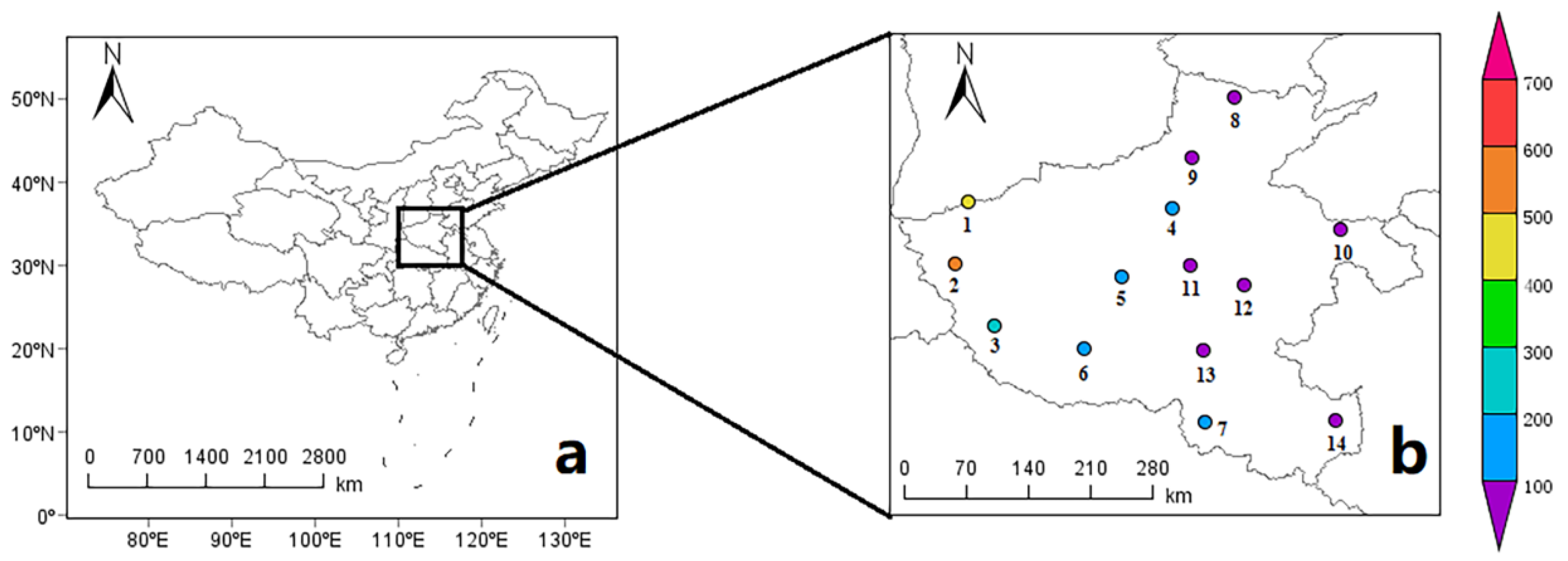
2.1. Datasets

This study utilized the monthly climate datasets of 14 stations in Henan Province (Figure 1 and

Table 1. The meteorological parameters (daily average value) of each station in Henan Province.

ID	Name	Latitude (DD)	Longitude (DD)	Elevation (m)	Region	Wind Speed	Relative Humidity	Air Temperature	Sunshine Hours
						(m/s)	(%)	(°C)	(h)
1	San menxia	34.8	111.2	409.9	Western part	2.4	62.6	14.1	7.7
2	Lu shi	34.1	111.0	568.8	Western part	1.4	69.9	12.7	7.4
3	Xi xia	33.3	111.5	250.3	Western part	2.1	70.7	15.3	7.3
4	Zheng zhou	34.7	113.7	110.4	Central part	2.5	65.9	14.7	7.3
5	Baofeng	33.9	113.1	136.4	Central part	2.6	77.2	14.7	7.2
6	Nan yang	33.0	112.6	129.2	Central part	2.2	71.7	15.2	7.1
7	Xin yang	32.1	114.1	114.5	Central part	2.3	74.1	15.5	7.3
8	An yang	36.1	114.4	62.9	Eastern part	2.3	65.2	14.1	7.6
9	Xin xiang	35.3	113.9	73.2	Eastern part	2.2	69.9	14.5	7.5
10	Shang qiu	34.5	115.7	50.1	Eastern part	2.5	71.5	14.3	7.5
11	Xu chang	34.0	113.9	66.8	Eastern part	2.4	69.5	14.7	7.2
12	Xi hua	33.8	114.5	52.6	Eastern part	2.2	72.0	14.7	7.4
13	Zhu madian	33.0	114.0	82.7	Eastern part	2.3	73.2	15.1	7.2
14	Gushi	32.2	115.6	42.9	Eastern part	2.7	76.2	15.6	7.4

). The monitoring stations are located in different topographies and elevations. For instance, the San menxia, Lu shi, and Xi Xia stations are in the western Henan Province with mountain topography and high elevation (elevation > 200 m); the Zheng zhou, BaoFeng, Nan yang, and Xin yang stations are in the central Henan Province with medium elevation (200 m > elevation > 100 m); the An yang, Xin Xiang, Shang Qiu, Xu chang, Xi Hua, Zhu madian, and Gushi stations are in the eastern Henan Province with plain terrain and low elevation (elevation < 100 m).

The monthly mean values of the solar radiation (Ro), relative humidity (RH), wind speed (W), air temperature (T), pan evapotranspiration (E), and sunshine duration (H) were used in this study for 53 years (from 1961 to 2013). The device of pan evapotranspiration is U20 type evaporator with a diameter of 0.20 m, depth of 0.10 m. The datasets were obtained from the China meteorological information center [26,27,28].

2.2. Models and Evaluation Criteria

2.2.1. Multiple Hidden Layer Back-Propagation (BP) Neural Network (MBP)

The back-propagation (BP) neural network was a feedforward neural network [29]. The main characteristic of the BP neural network was that the signal was forward feedback and the error was backpropagation. Prior to transmission, the input signal was processed step by step from the input layer to the hidden layer. Neurons state of each layer affected only the next layer. If the result layer did not get the desired output, the weight and threshold were adjusted based on the prediction error. BP neural network prediction results were constantly close to the expected forecast results.

The BP neural network was composed of an input layer, a hidden layer, and output layer. Hidden layers can be divided into a haploid hidden layer and multiple hidden layers according to the number of layers. Multiple hidden layers consisted of multiple single hidden layers. The multi-hidden layer had stronger generalization ability and higher prediction accuracy. The selection of hidden layer amounts should consider the network precision and training time comprehensively. For a simpler mapping relationship, the single hidden layer can be selected to improve the accuracy of the network. For complex mapping relationships, multiple hidden layers can be selected. In that regard, the multiple hidden layer BP neural network (MBP) was utilized in the current study.

2.2.2. Generalized Regression Neural Network (GRNN)

The generalized regression neural network (GRNN) was one of the radial base neural networks [30,31]. The GRNN had strong nonlinear mapping capability and a flexible network structure. The GRNN had higher fault tolerance and robustness. It was suitable for solving nonlinear problems. The GRNN had obvious advantages in approximation ability and learning speed. The GRNN can be converged to the optimal return along with the increase of samples. In addition, the GRNN can also deal with unstable data. Therefore, the GRNN had been widely used in signal processing, configurable analysis, and control decision system.

2.2.3. Probabilistic Neural Networks (PNN)

The probability neural network (PNN) was a feedforward neural network developed based on radial-based function [32,33]. Its theoretical foundation was the Bayesian minimum risk criterion and the probability of Parzen windows. The layers of the PNN were made up of input patterns, sum layers, and output layers. In practice, it had advantages of adopting a linear learning algorithm to complete the nonlinear problems with high precision. The corresponding weight of PNN was the distribution of design samples. The PNN network did not require drilling and can meet the real-time processing requirements.

2.2.4. Wavelet Neural Network (WNN)

The wavelet neural network (WNN) was based on the BP neural network topology. It was a feedforward recursive network with little pokey functions as the hidden nodes [34,35]. The wavelet base function used in this study was the Morlet wavelet function. It was similar to the BP neural network weight correction algorithm. It used a gradient correction method to calculate network weight and wavelet base function parameters and obtain the desired results of the wavelet neural network closer.

2.2.5. Stephens and Stewart Model (SS)

The Stephens and Stewart (SS) model was a simple linear regression function [10]. The equation can be indicated as E = Ro·(a₁ + b₁·T), where a₁ and b₁ are decided by training data utilizing the least square method.

2.2.6. Evaluation Criteria

The performance of neural networks and the empirical model were evaluated based on the root mean square error (RMSE) (Equation (1)), mean absolute error (MAE) (Equation (2)), coefficient of determination (R²) (Equation (3)), and Nash–Sutcliffe efficiency (E_N) (Equation (4)).

$$\mathrm{RMSE}=\sqrt{\frac{1}{\mathrm{N}}{{\displaystyle \sum }}_{\mathrm{i}=1}^{\mathrm{N}}{({\mathrm{E}}_{\mathrm{m},\mathrm{i}}-{\mathrm{E}}_{\mathrm{o},\mathrm{i}})}^2}$$

(1)

$$\mathrm{MAE}=\frac{1}{\mathrm{N}}{\displaystyle \sum }_{\mathrm{i}=1}^{\mathrm{N}}\left|{\mathrm{E}}_{\mathrm{m},\mathrm{i}}-{\mathrm{E}}_{\mathrm{o},\mathrm{i}}\right|$$

(2)

$${\mathrm{R}}^2=\frac{{({{\displaystyle \sum }}_{\mathrm{i}=1}^{\mathrm{N}}\left({\mathrm{E}}_{\mathrm{m},\mathrm{i}}-\overline{{\mathrm{E}}_{\mathrm{m}}}\right)\left({\mathrm{E}}_{\mathrm{o},\mathrm{i}}-\overline{{\mathrm{E}}_{\mathrm{o}}}\right))}^2}{{{\displaystyle \sum }}_{\mathrm{i}=1}^{\mathrm{N}}{({\mathrm{E}}_{\mathrm{m},\mathrm{i}}-\overline{{\mathrm{E}}_{\mathrm{m}}})}^2{{\displaystyle \sum }}_{\mathrm{i}=1}^{\mathrm{N}}{({\mathrm{E}}_{\mathrm{o},\mathrm{i}}-\overline{{\mathrm{E}}_{\mathrm{o}}})}^2}$$

(3)

$${\mathrm{E}}_{\mathrm{N}}=1-\frac{{{\displaystyle \sum }}_{\mathrm{i}=1}^{\mathrm{N}}{({\mathrm{E}}_{\mathrm{o},\mathrm{i}}-{\mathrm{E}}_{\mathrm{m},\mathrm{i}})}^2}{{{\displaystyle \sum }}_{\mathrm{i}=1}^{\mathrm{N}}{({\mathrm{E}}_{\mathrm{o},\mathrm{i}}-\overline{{\mathrm{E}}_{\mathrm{o}}})}^2}$$

(4)

where, N represents the number of variables, and the Em and the E_O are the modeled and observed values of pan evapotranspiration, respectively.

3. Results

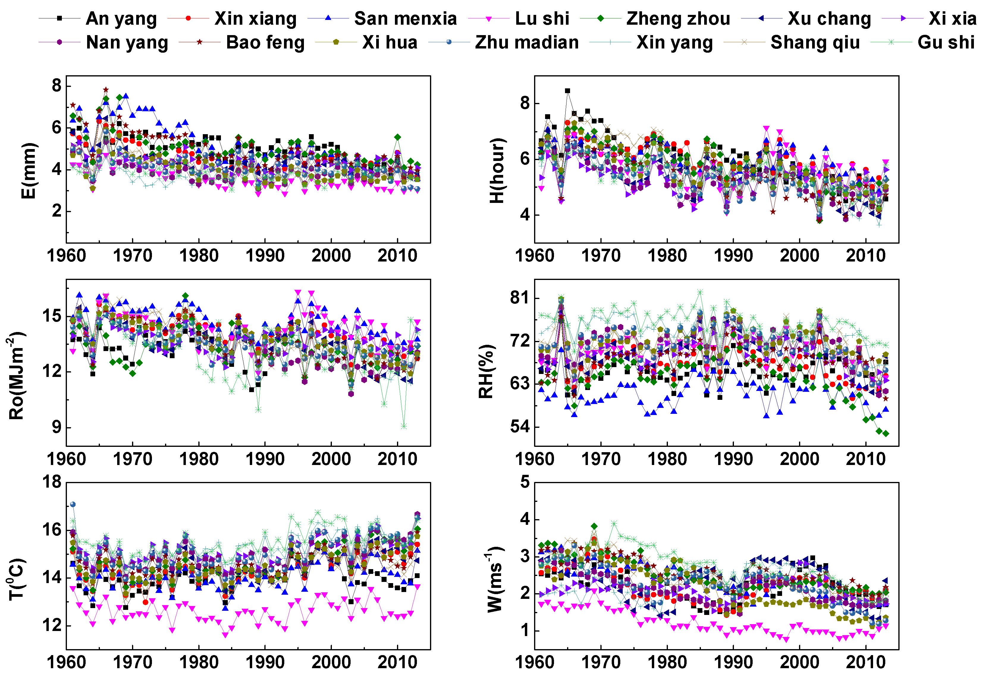
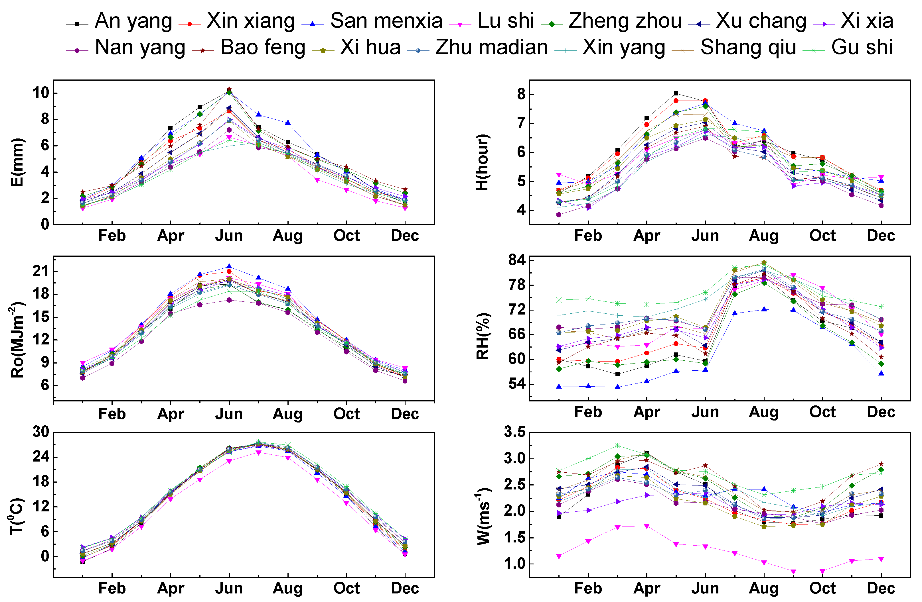
3.1. Interannual Variabilities of E

Figure 2 clearly shows the annual change of E and related climatic factors. From Figure 2, E values of San menxia, Zheng zhou, BaoFeng, and An yang stations were generally higher than those of other stations from 1961 to 2013. The tendencies of E values decreased slightly at every station from 1961 to 2013. The H values of Nan Yang, Xin Yang, and Xi Xia stations were relatively low and H monthly mean values of An yang, Xin xiang, and San menxia stations were high. The H values of all stations also showed downward trends. The R_o monthly mean values were high at San menxia, Lu shi stations, and low at Gushi, An yang, and Nan yang stations. The R_o values slightly decreased from 1961 to 1990, but slightly increased from 1990 to 2013. RH values of Gushi and Xin yang stations were generally greater than 72%, while RH values of San menxia stations were lower than 62%. Lu shi station had relatively lower T values than other stations; T values of Lu shi were generally lower than 13 °C, while T values of Gushi were generally above 15 °C. Meanwhile, W values were highest in Gushi station and lowest in Lu shi station. W values also showed downward trends at most stations from 1961 to 2013.

Figure 3 further illustrates the monthly variation of E and climatic parameters at each station. For example, the monthly changes of E, H, Ro, RH, and T are generally higher in summer, while the monthly changes of E, H, Ro, RH, and T are lower in winter. Differences in parameters at diverse observation stations revealed that the stations are typical in the study of E in different geographical regions of Henan province.

Table 2. Monthly mean values of meteorological variables for each observation station.

Station	Parameter	M	S	V	Skew	Min	Max	R
San menxia	Ro	14.69	5.12	26.2	0.14	5.43	25.32	0.93
	T	14.02	9.55	91.2	−0.14	−3.55	29.17	0.82
	H	6	1.59	2.52	0.13	1.94	10.11	0.8
	W	2.35	0.6	0.36	0.58	1.05	5.53	0.38
	RH	61.06	10.87	118.19	−0.24	30.14	88.37	−0.05
	E	5.18	3.11	9.65	0.84	0.88	16.75	1
Lu shi	Ro	14.26	4.68	21.88	0.23	6.02	25.29	0.94
	T	12.62	9.15	83.77	−0.12	−4.11	27.52	0.85
	H	5.64	1.51	2.27	0.09	1.91	9.76	0.64
	W	1.24	0.47	0.22	0.48	0.23	2.74	0.35
	RH	70.09	9.65	93.19	−0.51	41.39	90.39	−0.03
	E	3.46	2.04	4.17	0.69	0.58	10.24	1
Xi xia	Ro	13.75	4.63	21.46	0.12	5.3	24.54	0.94
	T	15.16	8.68	75.39	−0.11	−1.55	29.14	0.85
	H	5.28	1.48	2.18	0.02	1.3	9.55	0.8
	W	2.12	0.4	0.16	0.36	0.65	3.86	0.34
	RH	69.32	9.86	97.13	−0.62	27.45	90.33	−0.07
	E	4.16	2.13	4.54	0.78	0.84	12.66	1
Zheng zhou	Ro	13.29	4.36	19.04	0.14	4.51	23.7	0.89
	T	14.59	9.62	92.48	−0.14	−3.35	30.13	0.78
	H	5.84	1.65	2.71	0.05	1.63	10.38	0.82
	W	2.52	0.7	0.49	0.97	1.07	6.49	0.21
	RH	64.53	11.33	128.32	−0.27	29.74	87.77	−0.12
	E	4.98	2.73	7.47	1.01	0.9	16.07	1
Baofeng	Ro	13.62	4.76	22.63	0.14	4.97	24.16	0.88
	T	14.62	9.37	87.78	−0.11	−3.06	30.17	0.75
	H	5.39	1.61	2.59	0.1	1.54	9.67	0.81
	W	2.6	0.62	0.38	0.52	1.16	6.15	0.33
	RH	67.77	11.03	121.57	−0.45	23.58	90.83	−0.17
	E	4.99	2.71	7.33	1.19	0.93	17.06	1
Nan yang	Ro	12.31	4.21	17.75	0.04	4.83	23.18	0.95
	T	15.08	9.15	83.78	−0.12	−1.77	29.82	0.87
	H	5.2	1.61	2.59	0.14	1.29	9.75	0.8
	W	2.13	0.55	0.3	0.54	0.74	4.03	0.14
	RH	71.85	8.64	74.68	−0.55	40.48	90.48	−0.07
	E	3.7	2.05	4.19	0.73	0.66	11.13	1
Xin yang	Ro	13.51	4.57	20.89	0.18	4.73	24.2	0.95
	T	15.41	8.88	78.81	−0.13	−2.15	29.96	0.86
	H	5.29	1.62	2.63	0.23	1.18	10.49	0.8
	W	2.31	0.57	0.32	0.1	0.74	3.96	0.19
	RH	74.2	7.78	60.5	−0.6	49.97	90.32	−0.04
	E	3.64	1.9	3.6	0.61	0.61	10.25	1
An yang	Ro	13.19	4.5	20.24	0.13	4.28	23.21	0.94
	T	13.95	10.05	100.98	−0.17	−4.21	29.37	0.84
	H	6.07	1.82	3.3	0	1.02	10.87	0.79
	W	2.23	0.66	0.44	0.33	0.83	4.24	0.42
	RH	65.59	10.93	119.48	−0.14	37.52	88.81	−0.13
	E	4.98	2.93	8.58	0.52	0.66	13.52	1
Xin xiang	Ro	14.12	5.07	25.74	0.02	3.93	24.26	0.94
	T	14.36	9.74	94.86	−0.15	−3.27	29.34	0.79
	H	6.06	1.66	2.76	−0.16	1.28	9.93	0.8
	W	2.21	0.65	0.42	0.68	0.78	4.63	0.23
	RH	67.07	10.35	107.19	−0.28	35.23	87.94	−0.06
	E	4.48	2.39	5.72	0.68	0.66	13.09	1
Shang qiu	Ro	13.87	4.87	23.67	0.1	4.06	25.39	0.94
	T	14.23	9.62	92.58	−0.13	−4	29.42	0.81
	H	5.89	1.71	2.91	0.17	1.35	10.79	0.76
	W	2.46	0.7	0.49	0.59	1.01	5.66	0.34
	RH	71.47	9.62	92.56	−0.35	39.48	90.55	−0.12
	E	4.11	2.47	6.11	0.94	0.58	14.62	1
Xu chang	Ro	13.5	4.79	22.92	0.08	4.22	23.69	0.93
	T	14.69	9.41	88.54	−0.12	−2.6	30.01	0.83
	H	5.46	1.62	2.63	0.01	1.04	9.49	0.81
	W	2.33	0.67	0.45	−0.04	0.68	4.25	0.14
	RH	69.32	10.29	105.79	−0.5	32.13	89.81	−0.07
	E	4.32	2.39	5.71	0.8	0.78	12.77	1
Xi hua	Ro	13.79	4.83	23.33	0.08	4.67	24.72	0.92
	T	14.55	9.37	87.85	−0.12	−2.92	29.55	0.82
	H	5.71	1.64	2.69	0.08	1.72	10.44	0.78
	W	2.16	0.77	0.6	0.4	0.56	4.65	0.24
	RH	72.17	9.55	91.22	−0.61	36.9	90.23	−0.05
	E	3.85	2.27	5.15	1.02	0.67	16.66	1
Zhu madian	Ro	13.44	4.49	20.18	0.15	4.82	23.76	0.93
	T	15.09	9.18	84.36	−0.13	−3.21	30.01	0.84
	H	5.35	1.52	2.3	0.15	1.37	9.6	0.79
	W	2.26	0.62	0.38	0.05	0.86	4.24	0.18
	RH	71.45	9.63	92.73	−0.55	37.35	90.97	−0.08
	E	4.03	2.22	4.94	0.73	0.58	12.74	1
Gushi	Ro	13.12	4.67	21.78	0.25	3.72	25.14	0.92
	T	15.56	8.98	80.73	−0.14	−1.98	30.15	0.86
	H	5.52	1.62	2.63	0.19	1.54	10.92	0.82
	W	2.73	0.65	0.42	0.17	1.16	4.76	0.08
	RH	76.1	7.31	53.4	−0.64	52.61	90.29	−0.07
	E	3.65	1.92	3.69	0.7	0.65	11.05	1

The units of R_o, T, H, W, and E are MJm⁻², °C, hour, ms⁻¹, and mm/day, respectively; M, S, V, Skew, min, max represent the mean, standard deviation, variance, skewness, minimum, and maximum values, respectively. R represents the correlation between E and the relevant meteorological factor.

showed the monthly mean values of the climate parameters of every station. M, S, V, Skew, min, max represent the mean values, standard deviation values, variance values, skewness values, minimum, and maximum values, respectively. R represents the correlation coefficient between E and corresponding meteorological parameters. The monthly averages of E were from 0.61 (Xin yang) to 16.75 mm (San menxia) with corresponding V values varying from 3.60 to 9.65. The minimum monthly values of E were about 0.58 mm while the maximum monthly values of E reached 17.06 mm. At the same time, the monthly climatological parameters changed a lot in every observation station. For instance, the monthly mean values of R_o at San menxia were from 5.43 to 25.32 MJm⁻²; the monthly mean values of T also varied from −4.11 to 27.52 °C. The statistical data of S and V of each parameter of the above stations also show different climatic characteristics.

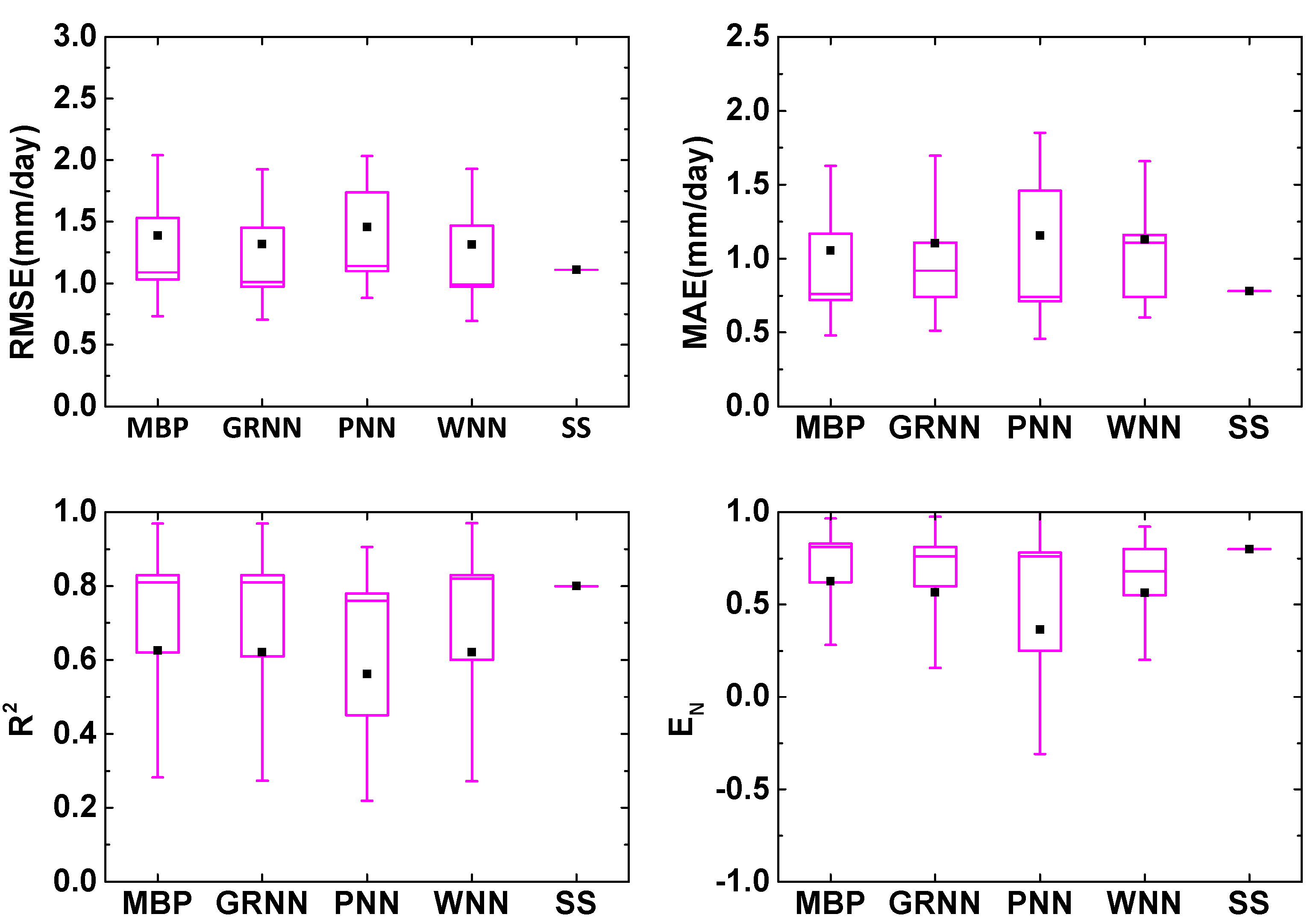
3.2. Prediction Results of Different ANN Models

This study tried different combinations of inputs.

Table 3. The input combination of different artificial neural network (ANN) models.

Models				Input Combination
MBP	GRNN	PNN	WNN
MBP 1	GRNN 1	PNN 1	WNN 1	Ro
MBP 2	GRNN 2	PNN 2	WNN 2	T
MBP 3	GRNN 3	PNN 3	WNN 3	H
MBP 4	GRNN 4	PNN 4	WNN 4	W
MBP 5	GRNN 5	PNN 5	WNN 5	RH
MBP 6	GRNN 6	PNN 6	WNN 6	Ro, T
MBP 7	GRNN 7	PNN 7	WNN 7	Ro, T, H
MBP 8	GRNN 8	PNN 8	WNN 8	Ro, T, H, W
MBP 9	GRNN 9	PNN 9	WNN 9	Ro, T, H, W, RH

provides an input combination for each model. Table S1 shows that the training and test results of MBP, GRNN, PNN, WNN, and SS models for predicting E of San menxia and Lu shi stations. From the table, the models with whole meteorological variables (Ro, T, H, W, and RH) had the optimum accuracy. In predicting E of San menxia, the WNN model is superior to other models. MBP model is superior to other models in the prediction of E at Lu shi. During the testing phase, the precision of the model was as follows WNN, GRNN, MBP, PNN, and SS in San menxia station. The accuracy level of the soft computing model in the test period was MBP, WNN, GRNN, PNN, and SS in Lu shi station. These accuracy levels are calculated based on the R², RMSE, MAE, E_N standards. Here, the WNN has the optimal precision, and the SS has the lowest precision at San menxia station. Additionally, MBP has the optimal precision while the SS also has the lowest precision in Lu shi. By comparing the simple two-input SS (R_o and T) model, the artificial neural network (ANN) models had better precision than the SS. Additionally, the two-input ANN computing models seem to have the same precision as the SS model in predicting E at San menxia and Lu shi stations. Table S2 shows the precision of applying models to predict E at Xi xia and Zheng zhou stations. Similar to Lu shi station, the all-weather input mode usually provides the best accuracy. The accuracy and optimal MBP model of Xi xia and Zheng zhou station in predicting E are better than the other models. The precisions ranks are MBP, GRNN, WNN, PNN, and SS. The precision of the two-input ANN models in predicting E at Xi xia and Zheng zhou station was the same as that of the SS model.

Table S3 provides the statistical data of the ANN model for predicting E at Baofeng and Nan yang stations. At Baofeng station, the performance of the five-input modes was the best, and the performance of the MBP model was better than that of other models. The accuracy ranks of models were as follows: MBP, WNN, GRNN, PNN, and SS. In Nan yang station, three-input MBP and two-input WNN models have better performance than their corresponding five-input models. The behavior of the GRNN is better than other models. The precision of the models is ranked as follows: GRNN, WNN, SS, MBP, and PNN. Obviously, compared with the two-input ANN model of Nan yang station, the effect of the SS model is poor. Table S4 reveals the results of Xin yang and An yang stations. It can be seen from those models with intact weather data that they usually have optimal accuracies. The WNN model has better behavior than the other models in Xin yang according to RMSE, MAE, R², and E_N. The rankings are WNN, MBP, GRNN, SS, and PNN in Xin yang. The MBP model has better behavior than others in An yang according to RMSE, MAE, R², and E_N. The rankings are MBP, GRNN, WNN, PNN, and SS in An yang. The SS model has the same precision as the two-input ANN models in predicting E at Xin yang and An yang station.

Table S5 shows the veracity of predicting E of Xin xiang and Shang qiu stations by using the ANN and experiential models. Similar to the previous stations, usually five-input models had optimal precisions, and the performance of the MBP model is superior to other models in RMSE, MAE, R², and E_N statistics. Accuracies of models in the test stage are ranked as follows: MBP, GRNN, WNN, PNN, and SS in both Xin xiang and Shang qiu stations. The accuracies of the MBP, GRNN, PNN, WNN, and SS models are shown in Table S6 for prediction E of Xu chang and Xi hua stations. Like previous sites, the five-input model typically provides the best performance. The five-input MBP model is both greater than the other models in Xu chang and Xi hua stations. The rankings of precisions are MBP, WNN, GRNN, SS, and PNN in Xu chang station. Additionally, in the Xi hua station, the accuracies are ranked as follows: MBP, WNN, GRNN, PNN, and SS. The comparison between the two-input models and SS model showed that the SS model had the same precision as other two-input ANN models in the test stage.

Table S7 provides the test accuracy of models for predicting E at Zhu madian and Gushi stations. In the two stations, the five-input ANN models also had the best precisions according to MAE, RMSE, R², and E_N index. The MBP model had optimal performance compared to the other models in predicting E at Zhu madian and Gushi stations. The performance ranks of the models both are MBP, GRNN, WNN, SS, and PNN at Zhu madian and Gushi stations. The comparison of two-input ANN models and SS models indicated that the two-input ANN models and SS models had similar performances. General precisions of models are shown in

Table 4. Accuracy rank ^a of the soft computing models in estimating pan evapotranspiration (E).

ID	Stations	MBP	GRNN	PNN	WNN	SS	Region
1	San menxia	3	2	4	1	5	Western part
2	Lu shi	1	3	4	2	5	Western part
3	Xi xia	1	3	4	2	5	Western part
4	Zheng zhou	1	2	4	3	5	Central part
5	Baofeng	1	3	4	2	5	Central part
6	Nan yang	4	1	5	2	3	Central part
7	Xin yang	2	3	5	1	4	Central part
8	An yang	1	2	4	3	5	Eastern part
9	Xin xiang	1	2	4	3	5	Eastern part
10	Shang qiu	1	2	4	3	5	Eastern part
11	Xu chang	1	3	5	2	4	Eastern part
12	Xi hua	1	3	4	2	5	Eastern part
13	Zhu madian	1	2	5	3	4	Eastern part
14	Gushi	1	2	5	3	4	Eastern part
	Total	20	33	61	32	64

^a Accuracy ranks were decided based on the RMSE, MAE, R², and E_N index. For the An yang station, for instance, BP has the highest precision (1st model) while the PNN has the lowest precision (4th model).

. The MBP model had much better scores than the other methods in predicting E and the final precisions are ranked as follows: MBP, WNN, GRNN, PNN, and SS. Additionally, the performance of GRNN and WNN were almost the same.

Figure 4 shows the comparison of models utilizing all stations database. Better accuracy appeared in five-input models. The MBP model was better than the other models. The precisions were ranked MBP, WNN, GRNN, PNN, and SS. Two-input MBP, WNN, GRNN models perform inferior to the SS model; the SS model has lower precision than the five-input ANN models (Figure 4 and

Table 5. The multiple hidden layer back propagation (MBP) model performances tested at different stations with full meteorological inputs (five-input).

ID	Stations	RMSE	MAE	R2	EN
1	San menxia	0.85	0.59	0.93	0.93
2	Lu shi	0.38	0.29	0.97	0.96
3	Xi xia	0.47	0.31	0.95	0.95
4	Zheng zhou	0.56	0.40	0.96	0.96
5	Baofeng	0.54	0.47	0.96	0.95
6	Nan yang	0.55	0.32	0.91	0.86
7	Xin yang	0.43	0.33	0.95	0.94
8	An yang	0.59	0.44	0.96	0.96
9	Xin xiang	0.46	0.34	0.96	0.96
10	Shang qiu	0.40	0.29	0.97	0.97
11	Xu chang	0.48	0.37	0.96	0.96
12	Xi hua	0.39	0.28	0.97	0.97
13	Zhu madian	0.38	0.30	0.97	0.97
14	Gushi	0.51	0.36	0.93	0.93

The unit of RMSE and MAE are mm/day.

). In Figure 4, all the ANN computing models generally have good generalization ability. The generalized MBP model was also tested at every site (Table 5). The results showed that the five-input MBP model had a high generalization ability based on RMSE, MAE, R², and E_N index.

4. Discussion

The Ro, T, and H were much better at modeling E than other variables in San menxia station. Table 2 shows the value of R also confirms this. Ro, T, and H parameters of Xi xia station also had a good performance in modeling E and is also shown in Table 2. In the Lu shi station, the R_o and T parameters were proved to be more valid in modeling E than H. This was because R_o (R = 0.94) had a higher correlation with E than H (R = 0.64) at Lu shi station. R_o proved to be the most valid variable in modeling E at Nan yang, Xin yang, Xu chang, and Gushi stations, which is also confirmed by the high R values. Models with W (or RH) generally provided worse results than those with R_o input. Adding W input generally decreased the model accuracies at Zheng zhou and BaoFeng stations (R = 0.21 in Zheng zhou and R = 0.33 in BaoFeng). Similar to the San menxia and Xi xia stations, the R_o input was found to be better at modeling E than the other input variables at An yang, Xin xiang, Shang qiu, Xi hua, and Zhu madian stations. Similar to the An yang and Xin xiang stations, the R_o variable had higher correlations with E (see Table 2) than H, W, and RH at Xi hua and Zhu madian stations. The T variable also provided better accuracy than the H, W, and RH in predicting E here.

Figure 4 also indicates that the R_o was the most useful variable in predicting E based on the all stations dataset. It is noteworthy that T and H input parameters were better. W and RH input parameters were worst. It was also indicated that only T or H input was deficient for high precision modeling E. The model behaviors were becoming better generally with the increase of input parameter amounts, which indicated that all meteorological variables had positive influences on modeling E in most of the stations of Henan Province. Some underestimations of ANN models also existed. Different geographical locations and climates may be the reason.

In short, ANN models with whole meteorological variables (R_o, T, H, W, and RH) generally had the best precision. This indicated that all these parameters are required for the best E model. The R_o was the most useful variable in modeling E from the all stations dataset. Then, T and H inputs parameters were better. W and RH input parameters were worst. Adding W or RH inputs into models usually weakens their precisions in modeling E in the all stations dataset. This reveals that the complicated nonlinear relationship between W (RH) and E cannot be shown from the ANN models we tested in this study. Two-input (R_o and T) ANN models usually provide better precision than the SS model in the all stations dataset. This told us that R_o and T can be preferred in some areas where obtaining the data of the other variables (H, W, and RH) are difficult.

Many ANN models, such as multi-layer perceptron (MLP), generalized regression neural network (GRNN), fuzzy genetic (FG), least-square support vector machine (LSSVM), multivariate adaptive regression spline (MARS), and adaptive neuro-fuzzy inference systems with grid partition (ANFIS-GP) have different accuracies in different climates. For example, the GRNN model performed better in Tibetan Plateau [2], however, SS models are preferred for some climatic zones such as BJ (Beijing), CQ (Chongqing), and HK (Haikou) stations [2] compared to the complex nonlinear models. Previous studies showed that ANN models are accurate, but their time efficiency is a little slower than the SS model. The adaptive neuro-fuzzy inference system (ANFIS) and ANN evaporation models also showed good performance when limited climatic parameters were used in the USA [3]. Shirsath et al. [9] also showed that ANN had slightly better performance than multiple linear regression (MLR) models, Penman, Priestley–Taylor, and SS [10]. Shiri et al. [10] showed that the gene expression programming (GEP) model was more accurate than empirical-physical models with improvements of adding gene thinking in the model [11]. It has been found that ANN worked very well at the study site in estimating evaporation in the hot and dry region [13]. The optimal COMBINE-GRNNM-GA method also had a good performance in predicting pan evaporation in the Republic of Korea by combining the advantages of both [17]. Comparing with ANN, the least squares-support vector, regression (LS-SVR), fuzzy logic, and adaptive neuro-fuzzy inference system (ANFIS) models revealed that machine learning models outperform the traditional Hargreaves and Samani method (HGS) and SS empirical methods [18]. We should choose appropriate ANN models in different regions of different climatic types. Such as, Ro, T, and H are the most useful variable of MBP in predicting E that we can choose in Henan Province (subtropical temperate continental climate). In the future, novel genetic algorithms of ANNs can be tried in predicting E, such as a stacking model that makes synergetic use of multiple ANN models can create more accurate and robust models [36,37]. Therefore, the ANN models of predicting pan evaporation have the advantage of efficiency and accuracy.

5. Conclusions

This study explored the abilities of four different ANN models, MBP, GRNN, PNN, and WNN, and one empirical SS model in modeling E utilizing different meteorological dataset combinations of Ro, T, H, W, and RH in Henan Province from 1961–2013. The climatic dataset obtained from 14 stations in different geographical locations were used as inputs for training and testing in Henan Province. The results of this study could be applied practically in the field of regional evaporation calculation. This study concluded that:

(a) ANN models with five-inputs generally have better accuracies (maximum R² = 0.96). The five-input ANN models provided better accuracy than the two-input (R_o and T) SS empirical model (R² = 0.80). Additionally, the two-input ANN models (maximum R² = 0.83) also generally performed better than the two-input (R_o and T) SS empirical model (R² = 0.80).

(b) The accuracies of the applied models rank as MBP (rank index: 20), WNN (rank index: 32), GRNN (rank index: 33), PNN (rank index: 61), and SS (rank index: 64). The MBP models are the most appropriate for predicting E using limited climatic inputs in different geographical locations and climatic zones in Henan Province. The performances of WNN and GRNN were almost the same.

(c) R_o seems to be the most important parameter in predicting E at most stations, while T and H inputs parameters were better. W and RH input parameters were worst. Adding W or RH inputs into models generally can increase model accuracies in predicting E.

References

1. Kim, S.; Shiri, J.; Singh, V.P.; Kisi, O.; Landeras, G. Predicting daily pan evaporation by soft computing models with limited climatic data. Int. Assoc. Sci. Hydrol. Bull. 2015, 60, 1120–1136. [Google Scholar] [CrossRef] [Green Version]
2. Wang, L.; Kisi, O.; Zounemat-Kermani, M.; Li, H. Pan evaporation modeling using six different heuristic computing methods in different climates of china. J. Hydrol. 2016, 544, 407–427. [Google Scholar] [CrossRef]
3. Shiri, J.; Dierickx, W.; Baba, P.A.; Neamati, S.; Ghorbani, M.A. Estimating daily pan evaporation from climatic data of the state of illinois, USA using adaptive neuro-fuzzy inference system (anfis) and artificial neural network (ann). Hydrol. Res. 2011, 42, 491–502. [Google Scholar] [CrossRef]
4. Adnan, S.; Ullah, K.; Khan, A.H.; Gao, S. Meteorological impacts on evapotranspiration in different climatic zones of pakistan. J. Arid Land 2017, 9, 144–158. [Google Scholar] [CrossRef] [Green Version]
5. Cheshmberah, F.; Zolfaghari, A.A. The effect of climate change on future reference evapotranspiration in different climatic zones of iran. Pure Appl. Geophys. 2019, 176, 3649–3664. [Google Scholar] [CrossRef]
6. Eslamian, S.; Khordadi, M.J.; Abedi-Koupai, J. Effects of variations in climatic parameters on evapotranspiration in the arid and semi-arid regions. Glob. Planet. Chang. 2011, 78, 188–194. [Google Scholar] [CrossRef]
7. Elahi, E.; Weijun, C.; Jhab, S.K.; Zhang, H. Estimation of realistic renewable and non-renewable energy use targets for livestock production systems utilising an artificial neural network method: A step towards livestock sustainability. Energy 2019, 183, 191–204. [Google Scholar] [CrossRef]
8. Eahi, E.; Weijun, C.; Zhang, H.; Abid, M. Use of artificial neural networks to rescue agrochemical-based health hazards: A resource optimisation method for cleaner crop production. J. Clean. Prod. 2019, 238, 117900. [Google Scholar]
9. Qiu, R.; Han, G.; Ma, X.; Xu, H.; Shi, T.; Zhang, M. A comparison of oco-2 sif, modis gpp, and gosif data from gross primary production (gpp) estimation and seasonal cycles in north america. Remote Sens. 2020, 12, 258. [Google Scholar] [CrossRef] [Green Version]
10. Shirsath, P.B.; Singh, A.K. A comparative study of daily pan evaporation estimation using ann, regression and climate based models. Water Resour. Manag. 2010, 24, 1571–1581. [Google Scholar] [CrossRef]
11. Shiri, J.; Marti, P.; Singh, V.P. Evaluation of gene expression programming approaches for estimating daily evaporation through spatial and temporal data scanning. Hydrol. Process. 2014, 28, 1215–1225. [Google Scholar] [CrossRef]
12. Martí, P.; González-Altozano, P.; López-Urrea, R.; Mancha, L.A.; Shiri, J. Modeling reference evapotranspiration with calculated targets. Assessment and implications. Agric. Water Manag. 2015, 149, 81–90. [Google Scholar] [CrossRef]
13. Piri, J.; Amin, S.; Moghaddamnia, A.; Keshavarz, A.; Han, D.; Remesan, R. Daily pan evaporation modeling in a hot and dry climate. J. Hydrol. Eng. 2010, 14, 803–811. [Google Scholar] [CrossRef]
14. Sharda, V.N.; Prasher, S.O.; Patel, R.M.; Ojasvi, P.R.; Prakash, C. Performance of multivariate adaptive regression splines (mars) in predicting runoff in mid-himalayan micro-watersheds with limited data/performances de régressions par splines multiples et adaptives (mars) pour la prévision d’écoulement au sein de micro-bassins versants Himalayens d’altitudes intermédiaires avec peu de données. Int. Assoc. Sci. Hydrol. Bull. 2008, 53, 1165–1175. [Google Scholar]
15. Kisi, O.; Shiri, J. Prediction of long-term monthly air temperature using geographical inputs. Int. J. Climatol. 2014, 34, 179–186. [Google Scholar] [CrossRef]
16. Majidi, M.; Alizadeh, A.; Farid, A.; Vazifedoust, M. Estimating evaporation from lakes and reservoirs under limited data condition in a semi-arid region. Water Resour. Manag. 2015, 29, 3711–3733. [Google Scholar] [CrossRef]
17. Kim, S.; Kim, H.S. Neural networks and genetic algorithm approach for nonlinear evaporation and evapotranspiration modeling. J. Hydrol. 2008, 351, 299–317. [Google Scholar] [CrossRef]
18. Goyal, M.K.; Bharti, B.; Quilty, J.; Adamowski, J.; Pandey, A. Modeling of daily pan evaporation in sub tropical climates using ann, ls-svr, fuzzy logic, and anfis. Expert Syst. Appl. 2014, 41, 5267–5276. [Google Scholar] [CrossRef]
19. Shiri, J.; Marti, P.; Nazemi, A.H.; Sadraddini, A.A.; Kisi, O.; Lenderas, G.; Fakherifard, A. Local vs. External training of neuro-fuzzy and neural networks models for estimating reference evapotranspiration assessed through k-fold testing. Hydrol. Res. 2015, 46, 72–88. [Google Scholar] [CrossRef]
20. Ki, Ö. Daily pan evaporation modelling using multi-layer perceptrons and radial basis neural networks. Hydrol. Process. 2010, 23, 213–223. [Google Scholar]
21. Chang, F.J.; Chang, L.C.; Kao, H.S.; Wu, G.R. Assessing the effort of meteorological variables for evaporation estimation by self-organizing map neural network. J. Hydrol. 2010, 384, 118–129. [Google Scholar] [CrossRef]
22. Kim, S.; Shiri, J.; Kisi, O. Pan evaporation modeling using neural computing approach for different climatic zones. Water Resour. Manag. 2012, 26, 3231–3249. [Google Scholar] [CrossRef]
23. Kisi, O. Pan evaporation modeling using least square support vector machine, multivariate adaptive regression splines and m5 model tree. J. Hydrol. 2015, 528, 312–320. [Google Scholar] [CrossRef]
24. Keskin, M.E.; Terzi, Ö.; Taylan, D. Fuzzy logic model approaches to daily pan evaporation estimation in western turkey/estimation de l’evaporation journaliere du bac dans l’Ouest de la Turquie par des modeles a base de logique floue. Int. Assoc. Sci. Hydrol. Bull. 2004, 49, 1010. [Google Scholar] [CrossRef]
25. Sanikhani, H.; Kisi, O.; Nikpour, M.R.; Dinpashoh, Y. Estimation of daily pan evaporation using two different adaptive neuro-fuzzy computing techniques. Water Resour. Manag. 2012, 26, 4347–4365. [Google Scholar] [CrossRef]
26. Zhang, Q.; Xu, C.Y.; Chen, X. Reference evapotranspiration changes in china: Natural processes or human influences? Theor. Appl. Climatol. 2011, 103, 479–488. [Google Scholar] [CrossRef]
27. Zhang, Q.; Xu, C.Y.; Chen, Y.D.; Ren, L. Comparison of evapotranspiration variations between the yellow river and pearl river basin, China. Stoch. Environ. Res. Risk Assess. 2011, 25, 139–150. [Google Scholar] [CrossRef]
28. Zhang, Q.; Qi, T.; Li, J.; Singh, V.P.; Wang, Z. Spatiotemporal variations of pan evaporation in china during 1960–2005: Changing patterns and causes. Int. J. Climatol. 2015, 35, 903–912. [Google Scholar] [CrossRef]
29. Sadeghi, B.H.M. A bp-neural network predictor model for plastic injection molding process. J. Mater. Process. Technol. 2000, 103, 411–416. [Google Scholar] [CrossRef]
30. Mantel, N. The detection of disease clustering and a generalized regression approach. Cancer Res. 1967, 59, 209–220. [Google Scholar]
31. Machado, R.N.D.M.; Bezerra, U.H.; Pelaes, E.G.; Oliveira, R.C.L.D.; Tostes, M.E.D.L. Use of wavelet transform and generalized regression neural network (grnn) to the characterization of short-duration voltage variation in electric power system. IEEE Lat. Am. Trans. 2009, 7, 217–222. [Google Scholar] [CrossRef]
32. Hornik, K.; Stinchcombe, M.; White, H. Multilayer feedforward networks are universal approxmations. Neural Netw. 1989, 2, 359–366. [Google Scholar] [CrossRef]
33. Araghi, L.F.; Hamid, K.; Arvan, M.R. Ship identification using probabilistic neural networks (pnn). Lect. Notes Eng. Comput. Sci. 2009, 2175, 18–22. [Google Scholar]
34. Zhang, Q.; Benveniste, A. Wavelet networks. IEEE Trans. Neural Netw. 1992, 3, 889–898. [Google Scholar] [CrossRef]
35. Chen, Y.; Yang, B.; Dong, J. Time-series prediction using a local linear wavelet neural network. Neurocomputing 2006, 69, 449–465. [Google Scholar] [CrossRef]
36. Arrieta, A.B.; Díaz-Rodríguez, N.; Del Ser, J.; Bennetot, A.; Tabik, S.; Barbado, A.; García, S.; Gil-López, S.; Molina, D.; Benjamins, R.; et al. Explainable artificial intelligence (xai): Concepts, taxonomies, opportunities and challenges toward responsible ai. Inf. Fusion 2020, 58, 82–115. [Google Scholar] [CrossRef] [Green Version]
37. Tsakiridis, N.L.; Tziolas, N.V.; Theocharis, J.B.; Zalidis, G.C. A genetic algorithm-based stacking algorithm for predicting soil organic matter from vis–NIR spectral data. Eur. J. Soil Sci. 2018, 70, 578–590. [Google Scholar] [CrossRef]
Figure 1. (a) The location of Henan province in China; (b) locations of weather stations in Henan Province (the color represents the height of each station). These stations were divided into three parts: western part (elevation > 200 m), central part (200 m > elevation> 100 m), and eastern part (elevation < 100 m) (Table 1).
Land 09 00229 g001
Figure 2. Annual variation trend of E and corresponding meteorological parameters of each station in Henan province.
Land 09 00229 g002
Figure 3. Seasonal variation trend of meteorological variables in each station.
Land 09 00229 g003
Figure 4. Statistics of different models at all stations.
Land 09 00229 g004