Article

Monitoring of Urban Landscape Ecology Dynamics of Islamabad Capital Territory (ICT), Pakistan, Over Four Decades (1976–2016)

1
Geospatial Research & Education Lab (GREL), Department of Space Science, Institute of Space Technology, Islamabad 44000, Pakistan
2
Freelance Journalist, Lahore 54000, Pakistan
*
Author to whom correspondence should be addressed.
Land 2020, 9(4), 123; https://doi.org/10.3390/land9040123
Submission received: 25 March 2020 / Revised: 15 April 2020 / Accepted: 16 April 2020 / Published: 20 April 2020
(This article belongs to the Special Issue Urban Ecosystem Services)

Abstract

:
In the late 1960s, the Islamic Republic of Pakistan’s capital shifted from Karachi to Islamabad, officially named Islamabad Capital Territory (ICT). In this aspect, the ICT is a young city, but undergoing rapid expansion and urbanization, especially in the last two decades. This study reports the measurement and characterization of ICT land cover change dynamics using Landsat satellite imagery for the years 1976, 1990, 2000, 2010, and 2016. Annual rate of change, landscape metrics, and urban forest fragmentation spatiotemporal analyses have been carried out, along with the calculation of the United Nations Sustainable Development Goal (SDG) indicator 11.3.1 Land Consumption Rate to the Population Growth Rate (LCRPGR). The results show consistent increase in the settlement class, with highest annual rate of 8.79% during 2000–2010. Tree cover >40% and <40% canopy decreased at an annual rate of 0.81% and 0.77% between 1976 to 2016, respectively. Forest fragmentation analysis reveals that ‘core forests of >500 acres’ class decreased from 392 km2 (65.41%) to 241 km2 (55%), and ‘patch forest’ class increased from 15 km2 (2.46%) to 20 km2 (4.54%), from 1976 to 2016. The LCRPGR ratio was 0.62 from 1976 to 2000, increasing to 1.36 from 2000 to 2016.

1. Introduction

The conversion of one land cover type to another is one of the most visible and rapid changes that the earth is experiencing and these conversions have profound social and environmental impacts at multiple scales. In the past, the drivers of land cover changes have been classified into two categories: proximate and distant, or indirect [1]. Recently, the phenomenon of tele-coupling between places has been recognized as key to understanding how distant drivers relate to proximate drivers and influence local landscape changes [2,3,4]. Some of the key drivers of landscape changes include economic, technological, institutional and policy, cultural, and demographic factors [5].
The growth of urban areas leads to land cover change in many parts of the world, especially in developing countries [3,6]. Intense urbanization and increase in anthropogenic activities reflect the scope, intensity, and frequency of human interference, and the changes they cause in ecological processes and systems in the urbanized areas [7]. The urban areas consist of only 1–6% of the earth’s land surface, yet they have enormous impacts on the functioning and service of local and global ecosystems, by modifying local climate conditions, eliminating and fragmenting native habitats, generating anthropogenic pollutants, etc. [8]. The spatial pattern of an urban landscape is a result of the interaction between various driving forces including natural and socioeconomic factors [9]. Increasing trends in industrialization and urbanization, along with the migration from rural to urban areas, are the most dominant factors influencing the land cover transformation. In the rural areas, employment opportunities and income are insufficient, which contributes to large differences in income and facility levels between urban and rural areas [10]. In developing countries, new cities are being developed due to human migration, infrastructure development, and growing job opportunities [10,11].
The United Nations (UN) Sustainable Development Goals (SDGs) are a collection of 17 global goals, which include 232 indicators set by the UN General Assembly for the year 2030. These goals are an urgent call for action by all countries—developed and developing—in a global partnership. Pakistan is a signatory to the UN SDGs, and this study analyzes the land use change dynamics of Islamabad Capital Territory (ICT) in the context of the relevant SDGs and indicators. The Goal 11 of the SDGs, “Make cities and human settlements inclusive, safe, resilient and sustainable”, with indicator number 11.3.1 “Ratio of Land Consumption Rate to Population Growth Rate (LCRPGR)” [12] is an important parameter for analyzing sustainability of land use and land change with population growth. The LCRPGR parameter is actually based on the previously defined parameters of LCR [13,14] and PGR [15], and several studies of urban areas have been carried out before on the basis of these parameters. The LCRPGR parameter and terminology has been given prime importance now after being linked with the UN defined SDGs. LCRPGR is vital to understand the rate of land change as compared to the population boom, to understand historical land consumption traditions, and to guide decision and policy makers on the planned expansion of the city along with the protection of environmental, social, and economic assets. Another SDG, Goal 15, “Protect, restore and promote sustainable use of terrestrial ecosystems, sustainably manage forests, combat desertification, and halt and reverse land degradation and halt biodiversity loss” emphasizes the protection of tree cover and sustainable management of forests. The SDG indicator number 15.2.1, "Progress towards sustainable forest management" [16] calls for sustainable management strategies for conserving the forest cover, enhancing environmental education, and engaging a wide range of stakeholder institutions, policies, regulations, and considerations that promote sustainability and utilization of natural resources at multiple spatial scales [17].
Assessment and monitoring of land cover dynamics is essential for the sustainable management of natural resources, environmental protection, biodiversity conservation, and developing sustainable livelihoods. Therefore, the development of applicable and systematic methods for producing and updating land cover databases are considered an urgent need [18]. Around the globe, urban land expansion rates are higher than or equal to urban population growth rates [19,20,21]. Many research studies focus on big cities and metropolises, where increase in population through analysis of census statistics is directly linked with the urban land expansion; however, these statistics do not provide information regarding spatial distribution, pattern, and scale of urban land use change. Multi-temporal land cover change analysis and simulation based on coarse to very high resolution satellite remote sensing images is becoming a well established technique for quantifying changes occurring on the earth’s surface, and multi-temporal aerial and satellite datasets are now widely and continuously being used for urban growth mapping, monitoring, and modeling with a focus on the spatial dimension and structures [22,23,24,25]. In urban expansion studies, spatiotemporal analysis of land cover and land use changes has helped towards understanding the underlying natural and socio-economic factors and drivers. For instance, Seto et al. [26] have presented a meta-analysis of 326 studies which used temporal satellite images to map urban land conversion. A total of 58,000 km2 increase in urban land area was reported in thirty years (1970 to 2000) and by 2030, global urban land cover is expected to increase between 430,000 km2 and 12,568,000 km2, with an estimate of 1,527,000 km2 more likely. According to Seto et al. [26], across all regions and for all three decades, urban land expansion rates are higher than or equal to urban population growth rates. Yang et al. [27] studied and reported the evidence of urban agglomerations through satellite images in four major bay areas of US (San Francisco and New York), China (Hong Kong-Macau), and Japan (Tokyo), from 1987 to 2017.
Clarke et al. [28] proposed a framework to combine remote sensing and spatial metrics for improved understanding and representation of urban dynamics to come up with alternative conceptions of urban spatial structure and change. Particularly with regards to urban forestry, a few studies have focused towards the assessment, mapping, and monitoring of urban forest parameters in fast-growing cities of developing countries. For example, Gong et al. [29] carried out a 30-year forest fragmentation study over Shenzhen Special Economic Zone (SEZ), a city which was established in 1979 in Southern China. Huang et al. [30] utilized satellite images of 77 metropolitan areas in Asia, US, Europe, Latin America, and Australia to calculate and analyze seven spatial metrics (area weighted mean shape, area weighted mean patch fractal dimension index, centrality, compactness index, compactness index of the largest patch, ratio of open space, and density). According to their analysis, the compactness, density, and regularity of urban areas in developing regions generally exceeded the levels reported throughout developed countries [30]. Dewan et al. [31] studied the dynamics of land use/cover changes though landscape fragmentation analysis in Dhaka Metropolitan, Bangladesh, computing and analyzing the following metrics: Number of patches, Patch density, Landscape shape index, Largest patch index, Mean patch size, Area-weighted mean fractal dimension, Interspersion and juxtaposition, Contagion, and Shannon’s diversity index.
In Pakistan, like other developing countries, most urban development is haphazard, typically lacking appropriate planning strategies [10]. Pakistan’s urbanization rate is the highest in South Asia, and by 2030, Pakistan will have more people in cities than in rural areas. Growing population and rapid development is causing prime agricultural land to be encroached and also causing loss of tree cover [32,33,34,35,36]. In the late 1960s, the capital of the Islamic Republic of Pakistan was shifted from Karachi to Islamabad (officially named Islamabad Capital Territory (ICT)). The masterplan of ICT was developed by the famous Greek architect and town planner C. A. Doxiadis [37]. In terms of a planned new capital, ICT is similar to planned new post-colonial capitals/relocations as in the cases of Brasilia (Brazil), Nur-Sultan (named as Astana from 1998 to 2019, and Akmola previously) in Kazakhstan, and Canberra (Australia) [38,39,40]. In the recent decades, with various ongoing development activities, ICT has been struggling with rapid urbanization and gigantic levels of pollution from industrial, residential, and transportation sources. In terms of population, ICT is considered as the most diverse city of Pakistan with a large percentage of immigrants and foreigner population [41]. Unprecedented influx of migrants and population increase has resulted in urban sprawl and conversion of fertile agricultural land and green cover into concrete—a clear deviation from the original ICT master plan [39,40]. Uncontrolled population growth in ICT due to rapid urbanization has deteriorated the living environment, and increased the adverse ecological impacts on human health, flora, and fauna [42].

1.1. Literature Review—ICT Mapping and Monitoring

In the last 20 years, several studies have been conducted on the ICT, regarding land cover change, biomass estimation, water quality monitoring, and temperature increase using satellite datasets. In this section, we present a synthesis of published work regarding land cover change dynamics in the ICT.
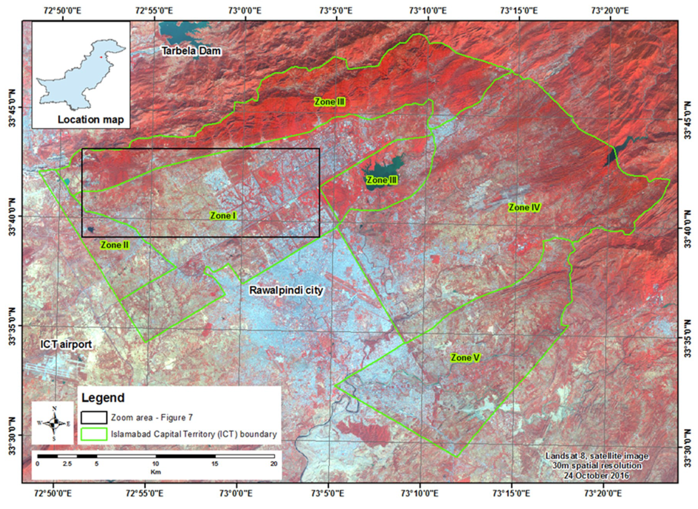
Adeel [43] identified urban growth potential through land use for ICT zone IV (Figure 1), based on SPOT-5 2.5 m panchromatic dataset and population census data, and found that nearly 63% of zone IV carries a ’High’ to ’Very High’ future growth potential, which is mainly located close to Islamabad Expressway. This work uses satellite imagery and field data from one year (2007) and does not report spatiotemporal change dynamics. Butt et al. [35] studied the metropolitan development in ICT, based on growth direction and expansion trends from the city center, for the period 1972–2009 using Landsat satellite images. Using Principal Components Analysis (PCA), band ratios, and supervised classification methods, they found that the urban development had expanded by 87.31 km2 in 38 years. Butt et al. [44] conducted a study on land cover change analysis over Simly dam watershed, ICT; the results derived from maximum likelihood supervised classification showed tree cover loss of up to 26% and 6% increase in settlements from 1992–2012, based on Landsat 5 TM and SPOT-5 imagery, respectively. Similarly, the watershed analysis of Rawal dam, ICT using Landsat 5 TM imagery, showed 3% degradation of tree cover and 2% gain of settlement from 1992–2012 [45]. Another ICT land cover change dynamics study conducted by Hassan et al. [46] utilized 30 m Landsat 5 TM data for 1992 and 2.5 m SPOT-5 data for 2012, using the maximum likelihood algorithm for image classification. The study revealed a decrease in forest cover of approximately 49% and over 213% gain of settlement area from 1992–2012. Sohail et al. [47] conducted a study to assess the water quality index and analyze the major change in land cover types, vegetation cover, rate of urbanization and its possible impact on groundwater resources, vegetation, and barren land. They used Landsat images for the years 1993, 1997, 2002, 2007, 2013, and 2017 for the assessment and mapping of land cover dynamics; according to their findings, from 1993 to 2017, vegetation areas decreased by 101.77 km2, surface water was reduced by 1.10 km2, barren land was reduced by 2.90 km2, while built-up lands expanded by 105.77 km2.
A comparison of Beijing, China and ICT for the role of vegetation in “controlling the eco environmental conditions for sustainable urban environment” was performed by Naeem et al. [42], where they used Gaofen-1 (GF-1) and Landsat-8 Operational Land Imager (OLI) satellite imagery with 8 m and 30 m spatial resolution, respectively. They evaluated various scenarios and models for future development to predict future spatial patterns in both cities. Another study was conducted by Naeem et al. [48] to study the association between green space characteristics, analyzed through landscape metrics, and land surface temperature for sustainable urban environments comparing Beijing, China and ICT.
Khalid et al. [49] conducted a study to quantify the decline of forest reserves and associated temperature variations in a relatively unexplored biodiversity hotspot of ICT, the Margalla Hills National Park (MHNP). In this work, Landsat satellite imagery from 1992, 2000, and 2011 was used to monitor the changes in forest cover and statistical significance tests were used to determine the significance of temperature variation associated with a shift in land cover classes. The study finds that deforestation and forest degradation by local communities is an ongoing practice in MHNP; this necessitates the promotion of conservation practices to minimize ecological disturbances here [49]. Batool and Javaid [50] carried out a study on the assessment of Margalla Hills forest by using Landsat imagery for years 2000 and 2018, and report that the forest cover has decreased from 87% in 2000 to 74% in 2018, whereas built-up area has increased from 5% in 2000 to 7% in 2018, and open land in the study area increased from 2% in 2000 to 7% in 2018. Mannan et al. [51] conducted a study using Landsat imagery, Markov Chain, and Cellular Automata on Margalla Hills, focusing on the quantitative assessment of spatiotemporal land use and land cover changes during 1998, 2008, 2018, and a simulation of 2028. In addition, a forest inventory survey was conducted for biomass and carbon sink estimations. This work shows that the forest area has reduced from 409.36 km2 to 392.31 km2 and settlement area has increased from 14.97 km2 to 39.66 km2 from 1998 to 2018. The average yearly biomass and carbon losses were 50.34 Gg/ha/yr and 31.33 Gg C/ha/yr, respectively.
The ICT is a relatively new and spatially heterogeneous city surrounded by the Himalaya mountainous dense forest as compared to other fast growing and expanding cities like Dhaka, Bangladesh [31,52,53,54,55], New Delhi, India [56], Beijing, China [42,48,57,58], Shanghai, China [59,60,61], Tokyo, Japan [27,62], etc. Based on the literature review, we observed that most studies of the ICT land cover dynamics have used different remotely sensed data, methods, definitions, and classification schemes, and have provided diverse results. Most studies which have analyzed the land change dynamics in the ICT focus on the overall analysis of land-cover and land-use change, and a detailed analysis of the landscape ecology and urban forestry characteristics is missing. There has further been very little focus in these studies towards urban landscape metrics and indicators of sustainable urban growth such as LCRPGR.

1.2. Study Objectives

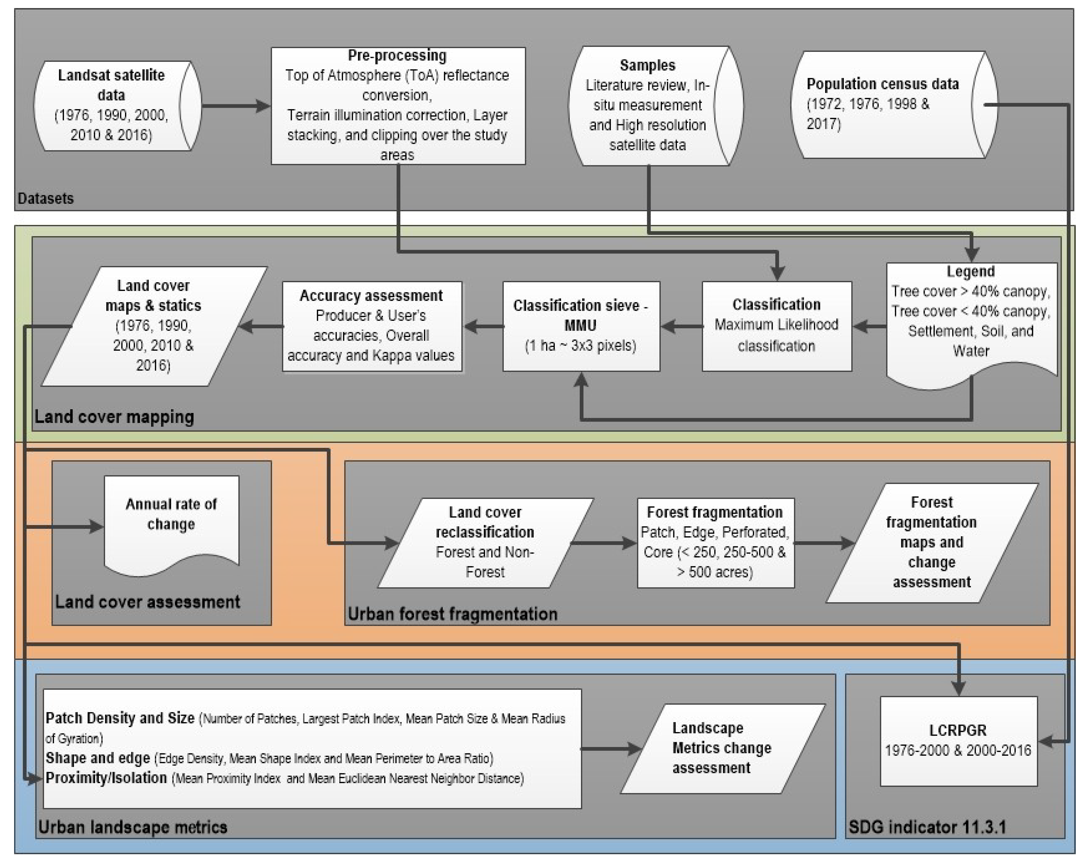
In this paper, well established, proven, and articulated research methodology, satellite datasets, and definitions of features were adopted with the goal to systematically achieve the following defined objectives:
  • Detection, measurement, and characterization of land cover features using Landsat medium resolution freely available satellite data (1976, 1990, 2000, 2010, and 2016) and determine the annual rate of change in land cover classes at 10 years interval.
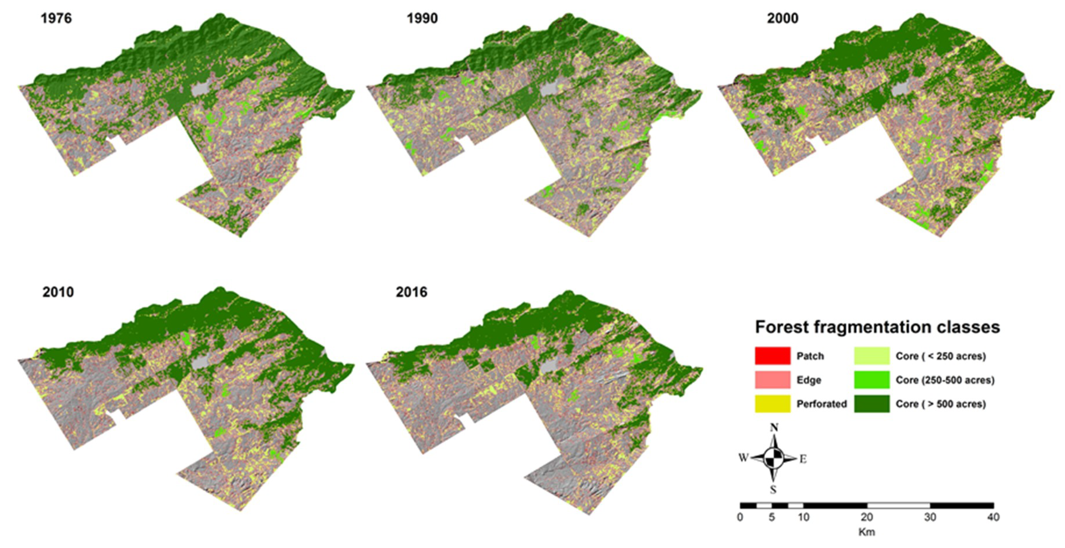
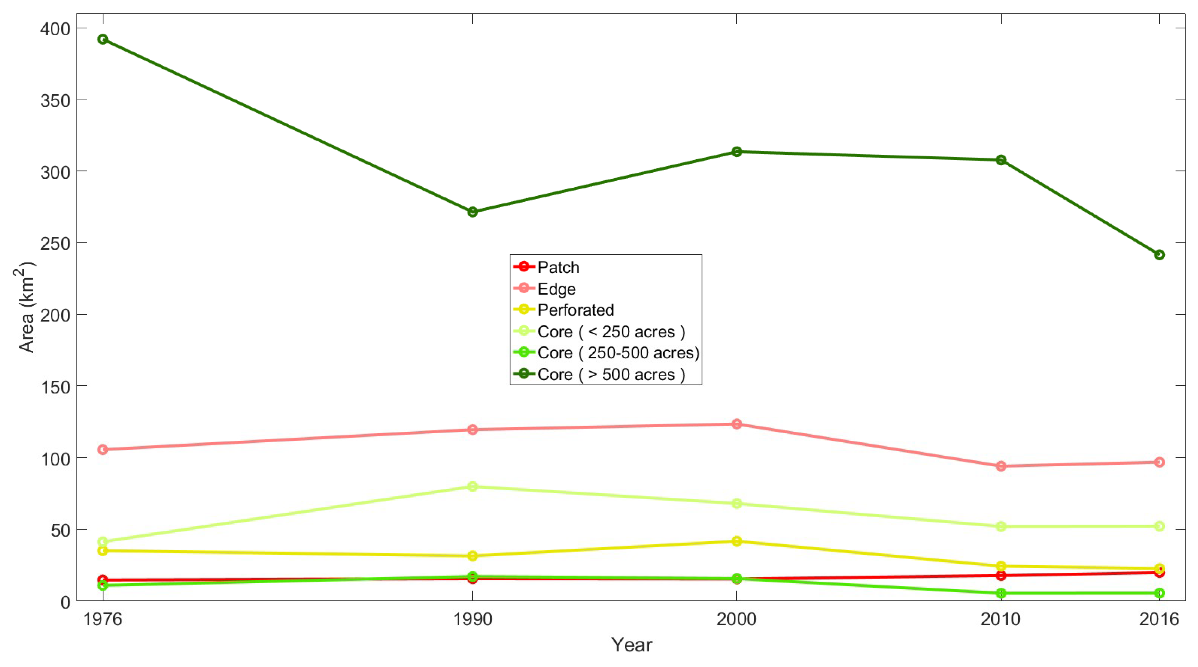
  • Landscape metrics and forest fragmentation spatiotemporal analysis, to estimate and report changes in the ICT urban ecosystem over forty years.
  • Calculation of SDG indicator number 11.3.1 “Land Consumption Rate to the Population Growth Rate (LCRPGR).”

2. Study Area

The ICT is the capital city of Islamic Republic of Pakistan (Figure 1) located in the Potohar plateau. It comprises an area of 906 km2 including mountains and uneven plains exceeding 1,175 m in height above the mean sea level [63]. According to the 2017 national population census, the total population of ICT is approximately two million, which makes it the ninth largest city of Pakistan. It has a humid and sub-tropical climate with four distinct seasons: autumn, spring, summer, and winter. The temperatures vary from 13 °C in January to 38 °C in June. ICT consists of five planning zones: Zone I, II, and V are reserved for planned urban development, while the remaining two zones, III and IV, are managed as National Park and the rural fringes. Marble and chemical factories, steel mills, flour mills, oil units, pigments, paints, and pharmaceutical manufacturing plants are some of the main industries in the city [34].

3. Materials and Methods

3.1. Datasets

To study the land cover dynamics and spatial analysis of ICT, various datasets have been collected from primary and secondary sources. The data collected from the primary sources include Landsat medium resolution satellite imagery and field observations using Geographical Positioning System (GPS) receiver, while the secondary or ancillary data consist of population census and ground truth data from Very High Resolution Satellite (VHRS) imagery.

3.1.1. Landsat Satellite and Digital Elevation Model (DEM) Data

For land cover mapping, we used 30 m spatial resolution orthorectified and cloud free Landsat Multispectral Scanner System (MSS), Thematic Mapper (TM), Enhanced Thematic Mapper Plus (ETM+), and Operational Land Image (OLI) sensor images. The TM, ETM+, and OLI sensors have the same 30 m spatial resolution, while the MSS has a spatial resolution of 57 m. The overall ICT region is covered within one Landsat scene (185 × 185 km). A total of five images for years 1976, 1990, 2000, 2010, and 2016 were downloaded from the United States Geological Survey (USGS) Earth Resources Observation and Science (EROS) archive. All satellite data was collected for the months of October and November, to avoid cloud cover (Table 1).
A 30 m spatial resolution Shuttle Radar Topography Mission (SRTM) Digital Elevation Model (DEM) from USGS was used to understand the topography of the area and to prepare the study area maps.

3.1.2. Population Census Data

For the calculation of SDG Goal 11 indicator 11.3.1 LCRPGR, we used the data collected from secondary sources including demographic data (primary census abstracts for the year 1972, 1998, and 2017) from the Pakistan Bureau of Statistics. We used actual census data of 1972 and 1998 to determine the shape of the population curve, which was exponential, as expected. Using the fitted exponential regression function, we derived the growth rate through the exponential function derivative—Equation (1), and then Equation (2) was utilized to determine the approximate population for the year 1976. The population data used for the calculation of LCRPGR is given in Table 2.
Growth   rate = ( ab ) e ac
Pop 1976 = Pop 1972 + 4   ×   Growth   rate
where a and b are regression coefficients, c represents the population variable, POP1976 = Estimated Population in 1976, and POP1972 = Past Population in 1972.

3.1.3. Ground Truth Data

In this study, we collected ground truth data from two sources: the primary ground data was collected using a Global Positioning System (GPS) receiver in October 2016 during field survey at various locations of ICT, while for the secondary ground data we relied on sub-meter VHRS imagery from Google Earth. A total of 205 samples were gathered, which were utilized as reference data for the satellite image classification and accuracy assessment of results. Using the Google Earth temporal VHRS data, we visually identified and geo-tagged the sites witnessing land degradation, urban development, and tree loss. The geo-tagged dataset helped to validate Landsat-based land cover changes.

3.2. Methodology

Our methodology (Figure 2) on land cover assessment and spatial analysis of ICT consists of (i) pre-processing of Landsat images, (ii) classification of Landsat images, (iii) accuracy assessment of land cover products, (iv) temporal land cover assessment, (v) urban landscape metrics analysis, (vi) urban forest fragmentation analysis, and (vii) LCRPGR calculation.

3.2.1. Pre-Preprocessing Landsat Images

Pre-processing steps for Landsat images included Top of Atmosphere (ToA) reflectance conversion, terrain illumination correction, and layer stacking of spectral bands. A reduction in between-scenes variability was accomplished through normalization for solar irradiance with a two-step process. First, we converted all pixels’ Digital Numbers (DNs) to radiance values using the bias and gain values, which were scene-specific and given in the metadata file of the respective scene. Second, we converted radiance data to ToA reflectance [64]. Terrain illumination correction was conducted using an empirical rotation model proposed by Tan et al. [65]. Layer stacking was performed to construct multi-spectral images at 30 m spatial resolution. The false color composite (FCC) of bands 542 from the multi-spectral images was used to visually interpret land cover features.

3.2.2. Classification of Landsat Satellite Images

The image classification procedure is to instinctively categorize all pixels in an image into land cover classes [66]. In this study, the maximum likelihood classification method was used for land cover-mapping from Landsat images. The maximum likelihood classification method is a supervised classification technique, which works on the basis of multivariate normal probability density function of categories, and utilizes both the variance and co-variance of the spectral response of each unknown pixel to assign it to a particular category [67,68]. In this study, five land cover classes were specified: Tree cover >40% canopy, Tree cover <40% canopy, Settlement, Soil, and Water. Almost 35 training samples were collected for each land cover class to classify the various Landsat images. The classified objects with an area smaller than the Minimum Mapping Unit (MMU) (i.e., 1 ha ~ 3 × 3 pixels) were fused with the neighboring land cover classes [69]. We adopted on-scene digitization technique for land cover change detection. First, we overlaid 2016 base land cover map on the multi-spectral Landsat image of 2010. We traced patches where land changes had occurred, leaving unchanged patches unmodified for consistency [70]. We followed the similar approach to detect land cover change between 2000 and 2010, using 2010 land cover map as a base layer. This process was repeated to generate land cover change maps between 1976–1990, 1990–2000, 2000–2010, and 2010–2016.

3.2.3. Accuracy Assessment of Land Cover Products

Assessment of classification accuracy of 1976, 1990, 2000, 2010, and 2016 land cover maps was carried out to determine the quality of information derived from the data. Random sampling method was adopted to assess the accuracy of satellite derived land cover products. Accuracy was assessed using 125 reference points, based on ground truth data and satellite visual interpretation. The comparison of classification results and reference data was carried out statistically using error matrices. In addition, the non-parametric kappa statistic was computed for each classified map to measure the accuracy of results, as it not only accounts for diagonal elements but also for all elements in the confusion matrix [71].

3.2.4. Temporal Land Cover Assessment

In this study, within the 906 km2 total area of ICT, the land cover maps (1976, 1990, 2000, 2010, and 2016) were compared in terms of the area. According to Puyravaud [72], the annual rate of change is based on the compound interest law, considering non-linear change across the timeline to estimate the percentage change per year. In this study, the annual rate of change was calculated using Equation (3) proposed by Puyravaud [72].
r = ( 1 t 2 t 1 ) × ( ln   A 2 A 1 )   ×   100
where r is the annual rate of change in percentage, and A 1 and A 2 is the area at earlier time t 1 and later time t 2 , respectively, and ln denotes the natural logarithm function.

3.2.5. Urban Landscape Metrics Analysis

Landscape metrics are used in this study to quantify the spatial patterns of land cover categories. The landscape metrics can be defined as quantitative and comprehensive measurements showing spatial diversity at a specific scale and resolution [73,74]. In this study, landscape metrics analysis was performed at land cover class level to quantitatively analyze spatial structures and patterns of the topographically and biophysically heterogeneous and diverse landscape of the ICT [74].
Under the three habitat categories Patch Density and Size, Shape and Edge, and Proximity/Isolation, a total of nine landscape metrics were used to quantify structural changes: Number of patches (NP), Mean Patch Size (MPS), Largest Patch Index (LPI), Mean Radius of Gyration (MRG), Mean Shape Index (MSI), Edge Density (ED), Mean Perimeter to Area Ratio (MPAR), Mean Euclidean Nearest Neighbor Distance (MED), and Mean Proximity Index (MPI) (Table 3). The landscape metrics were calculated using the FRAGSTATS v4 software tool. The output of the landscape metric analysis depends upon the spatial resolution of the data [75]; in this particular study, 30 m spatial resolution data has been chosen from 1990 to 2015 and 60 m spatial resolution for 1976.

3.2.6. Urban Forest Fragmentation Analysis

Forest fragmentation is the splitting up of large contiguous forest fields into smaller or less contiguous areas. A number of events or activities can lead to forest fragmentation including road formations, woodcutting, forest conversion to agriculture, forest fires, and human conflict over forest patches [25]. To assess forest fragmentation in ICT, the land cover map is divided into two major categories: forest and non-forest. Forest class consists of tree cover greater and less than 40% canopy cover while non-forest class comprises of settlement, soil, and water land cover classes. The outcome of forest fragmentation analysis was represented into six categories: Patch, Edge, Perforated, Core (<250 acres), Core (250–500 acres), and Core (>500 acres). These categories are signs of forest ecosystem quality and can be used to estimate the amount of fragmentation present in a landscape and the potential habitat impacts [25,76].

3.2.7. Ratio of Land Consumption Rate to the Population Growth Rate (LCRPGR) Calculation

One of the goals of this study is the calculation of the SDGs indicator 11.3.1 Land Consumption Rate to the Population Growth Rate (LCRPGR), which aims at monitoring and measuring urban development by comparing the urban expansion rate with the population growth rate on similar temporal and spatial scales [12,77]. If the LCRPGR ratio value lies between 0 ≤ LCRPGR ≤ 1, it shows the simultaneous increase of population growth rate (PGR) and land consumption rate (LCR), but the land consumption rate is much slower than the population growth rate. On the other hand, if LCRPGR > 1, it reflects the simultaneous increase of PGR and LCR, with a faster LCR than the PGR. To estimate the LCRPGR, satellite data derived land cover maps were used for the years 1976, 1998/2000 and 2016/2017, and census data was used for the specific years (Table 2). The indicator 11.3.1 was assessed at the local level for ICT using the mathematical expressions currently proposed by UN-Habitat, given below in Equations (4)–(6) [77]:
LCRPGR   = Land   Consumption   Rate Population   Growth   Rate  
Land   Consumption   Rate = ln ( Urb t + n Urb t ) n
Population   Growth   Rate = ln ( Pop t + n Pop t ) n
where, ln = Natural logarithm, Ur b t + n = Surface occupied by urban areas at the final year (t + n). Ur b t = Surface occupied by urban area at the initial year (t), Po p t + n = Population living in urban areas at the final year (t + n), Po p t = Population living in urban areas at the initial year (t), and n = Number of years between the two time intervals.

4. Results

4.1. Accuracy Assessment of Land Cover Products

According to the confusion matrix analysis, 90% overall accuracy and kappa coefficient value of 0.85 was attained for the 2016 classified map. Similarly, overall classification accuracy levels of 88% with kappa coefficient of 0.84 for 2010, 86% with kappa coefficient of 0.82 for 2000, 85% with kappa coefficient of 0.81 for 1990, and 83% with kappa coefficient of 0.79 for 1976 image classifications were achieved (Table A1 in Appendix A).

4.2. Temporal Land Cover Assessment

The overall settlement in the ICT increased while tree cover classes (greater and less than 40% tree canopies) decreased in forty years (1976 to 2016). The estimated land cover area for each image is summarized in Table 4 and spatial distributions are presented in Figure 3.
The settlement class in ICT increased from 29.99 km2 (3.31%) in 1976 to 170.40 km2 (18.80%) in 2016. The tree cover >40% canopy class showed a slight increase, 182.87 km2 (20.18%) in 1976 to 192.19 km2 (21.21%) in 1990 and then declined to 132.27 km2 (14.59%) in 2016. Tree cover <40% canopy land cover class faced overall decline from 1976 to 2016: 417.03 km2 (46.02%) in 1976 to 342.94 km2 (37.85%) in 1990, increase from 1990 to 2000 to 399.31 km2 (44.07%), while again decreased from 2000 to 2016 to 306.53 km2 (35.72%). The other two land cover classes, soil and water, observed fluctuating trends in the forty year period. The soil area of 270.27 km2 (29.83%) in 1976 increased to 317.91 km2 (35.08%) in 1990 and then reduced to 257 km2 (28.37%) in 2000, then further decreased to 254.34 (28.02%) in 2010, and again increased to 289.45 km2 (33.82%) in 2016. The change in water area was not significant though it has shown fluctuations during the study period; it increased from 5.86 km2 (0.64%) in 1976 to 8.44 km2 (0.94%) in 1990, and to 10.51km2 (1.16%) in 2000, then decreased to 6.29 km2 (0.69%) in 2010, and then increased slightly to 6.51 km2 (0.76%) in 2016 (Table 4).
Based on the temporal land cover data in the ICT, urban landscape settlement increased at an annual rate of 4.34% since 1976, with the highest annual rate of 8.79% during 2000–2010. The tree cover >40% canopy decreased at an annual rate of 0.81% between 1976 to 2016 and tree cover >40% canopy declined at an annual rate of 0.77% in forty years (1976–2016). The tree cover >40% canopy witnessed the highest loss rate at 2.38% per annum between 2000–2010, and tree cover <40% canopy experienced tree cover loss at 2.72% during 2010–2016 (Table 5).

4.3. Urban Landscape Matrix Analysis

Landscape matrix analysis was performed at class level, and the results for each class are reported in Figure 4 and Table A2 in Appendix A. The parameters Number of patches (NP), Largest Patch Index (LPI), Edge Density (ED), and Mean Proximity Index (MPI) for the settlement class overall increased from 1976 to 2016. Largest Patch Index (LPI) increased to 16% in 1990 from 13% in 1976, and then reduced to less than 10% in 2000, 2010, and 2016. For tree cover greater than and less than 40% canopy, Number of patches (NP) and Edge Density (ED) initially increased from 1976 to 2000, and then declined from 2000–2016. For tree cover greater than and less than 40% canopy, soil, and settlement classes, the Mean Patch Size (MPS) and Mean Euclidean Nearest Neighbor Distance (MED) sharply declined from 1976 to 1990 and remained lower. In the Mean Euclidean Nearest Neighbor Distance (MED), tree cover greater than and less than 40% canopy, soil and settlement classes remained less than 250 m throughout from 1976 to 2016. From 1976 to 2010, the Mean Radius of Gyration (MRG) decreased for tree cover greater than and less than 40% canopy, and then slightly increased during the years 2010 to 2016. For tree cover >40%, the canopy Mean Proximity Index (MPI) slightly increased between 1976 to 2016 while for tree cover >40%, the canopy MPI decreased from 1976 to 1990, grew between 1990 to 2010, and then again sharply reduced from 2010 to 2016. In all the land cover classes, the Mean Shape Index (MSI) value remained greater than 1 with slight fluctuations. In the Mean Perimeter to Area Ratio (MPAR), the settlement class increased from 640 in 1976 to 1000 in 1990 with slight increase till 2016.

4.4. Urban Forest Fragmentation Analysis

The forest fragmentation analysis results are presented in Figure 5 and Figure 6, and Table A3 in Appendix A. The analysis shows that the overall core forests of >500 acres decreased from 391.98 km2 (65.41%) in 1976 to 241.44 km2 (40.29%) in 2016. In the forty years’ time span, the patch class increased to 20 km2 (4.54%) in 2016 from 14.74 km2 (2.46%) in 1976. The perforated forest fragmentation class was 35.21 km2 (5.88%) in 1976, which increased 41.79 km2 (7.23%) in 2000, and then again declined to 22.74 km2 (5.18%) in 2016. For the edge class, a minor increase was observed from 1976 to 2000 and then a drop in 2016.

4.5. Ratio of Land Consumption Rate to the Population Growth Rate (LCRPGR)

For the years 1976–2000, the LCRPGR ratio (SDG indicator 11.3.1) was obtained to be 0.62, which highlights the simultaneous increase of Population Growth Rate (PGR) and Land Consumption Rate (LCR), but the LCR is much slower than the PGR. For the years 2000–2016, the LCRPGR ratio was obtained to be 1.36, which reflects the simultaneous increase of PGR and LCR, with a faster LCR than PGR.

5. Discussion

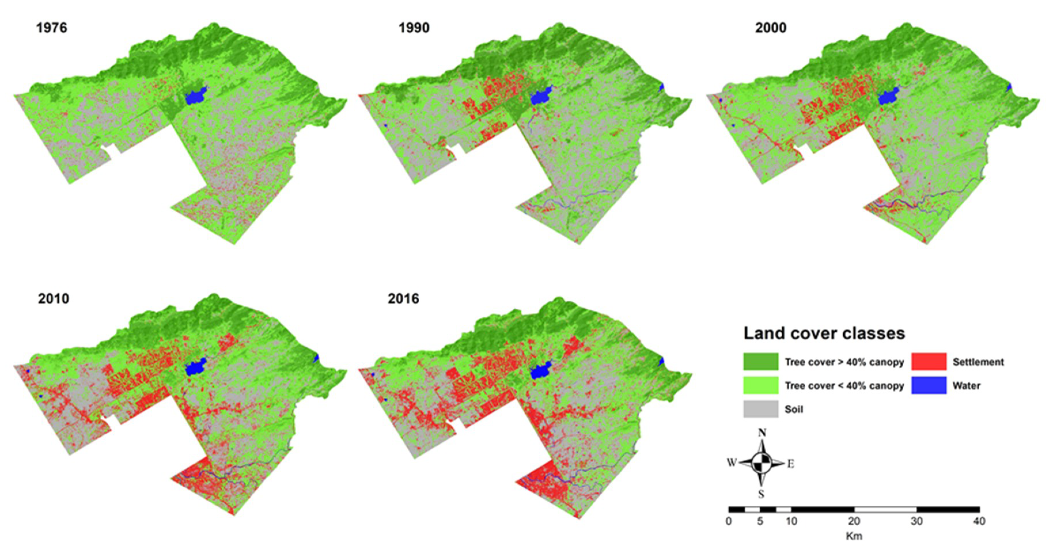
The present study was conducted in order to quantitatively analyze the landscape change dynamics in the ICT from 1976 to 2016 using medium spatial resolution Landsat images. In this study, we observed an increase in settlements over the last forty years. The dramatic land cover change in settlements is exerting severe pressure on other land cover classes, particularly tree cover and soil. Already existing urban areas can be seen expanding through rapid construction of residential blocks in the form of housing societies, industrial blocks and road expansions, leading to horizontal and vertical developments in the city and development of lavish farm houses in the vicinity areas (Figure 7). This rapid increase in urbanization is linked also with migrations. Urban growth may have positive or negative impacts on the environment but unplanned growth of urban areas has negative effects. For the economic development of the country, necessary planning is required to make urbanization helpful, as social, health, and environmental issues often accompany the process of urbanization.
In the time span of forty years, an overall decrease has been observed in the area of tree cover classes (i.e., greater than and less than 40% tree canopy) in the ICT, and most of the tree loss has occurred after the year 2000 with a corresponding increase in built-up areas. Apart from tree cutting, another important reason behind rapid tree loss or degradation is forest fires. In the Margalla Hills, forest fires usually take place during dry hot climate conditions when there is no rain for months and temperature goes up to 45 °C. According to Khalid and Ahmad [78], a total of 320 forest fires were recorded from 2002 to 2012 and approximately 8 km2 area got burnt as a result. In the ICT, due to uncontrolled urbanization and lack of awareness, huge tree loss has been observed in the last sixteen years, i.e., 2000–2016. Another factor for forest degradation is uncontrolled grazing of livestock [78]. As such, there are no adequate plans or manageable methods to stop grazing activities. For ecotourism and public awareness drives, a number of jogging and hiking trails have been formed in Margalla Hills National Park, and a large number of visitors has severely affected the Margalla Hills National Park by dumping waste. These illegal and unmonitored activities in the forested area cause threats to the forest ecosystem [50,79].
Massive migrations have occurred over the past few years from rural to urban areas, mostly due to low cultivated land output, landlessness, sub-division of land, poor economy, and better educational and health opportunities in urban areas. The rapid increase in population has contributed towards natural resource depletion and rapid deforestation close to settlements [80].
The LCRPGR parameter is an indicator of urban sustainable development, whether urban expansion is in balance with population growth or not. According to literature review, limited scientific peer reviewed studies have been reported on the monitoring and mapping of LCRPGR. Under each SDG, a number of targets and indicators have been defined, which countries have to quantify, but most of the developing countries do not have comprehensive databases through which they can compute, quantify, and report the SDGs indicators. To the best of the authors’ knowledge, only Nicolau et al. [77] and Wang et al. [81] have computed and reported scientific results of SDG proposed LCRPGR over urban areas. Nicolau et al. [77] based their study over the mainland of Portugal, while Wang et al. [81] carried out their study over mainland China, using earth observation and population census data, and reported the increase of LCRPGR value from 1.69 in 1990–2000 to 1.78 in 2000–2010. The LCRPGR related research findings from these studies show that in most cities, both horizontal and vertical urban expansions are carried out in an unplanned manner which has already effected the equilibrium of land consumption versus population increase to attain effective development goals by 2030 [77,81]. In this study over the ICT, the LCRPGR ratio was 0.62 from 1976 to 2000, which increased to 1.36 from 2000 to 2016. Based on studies conducted on the global scale, in the most of the cases LCR is higher than or equal to PGR due to high demand of luxurious occupancies in the urban areas [26,30].
The Shenzhen SEZ and ICT cities were both developed in late 1970s. In terms of urban forest cover change, Shenzhen SEZ had been restored to ~85% (1973–2005) [29] while in this study, we detected urban forest loss of ~27% (1976–2016) in the ICT. In both cities (SEZ and ICT), urban forest fragmentation results revealed losses in forest patches. In South Asia, the landscape of the ICT resembles strongly with the cities of Kathmandu (the capital of Nepal) and Thimphu (the capital of Bhutan), as they are all cities topographically surrounded by the pine trees. As compared to ICT, Kathmandu and Thimphu cities are older but highly migrant resident populated, vastly encroached, and over grazed. Although many studies have investigated the land cover dynamics of Kathmandu and Thimphu cities using temporal satellite data [82,83,84,85], detailed analysis using parameters such as landscape metrics, forest fragmentation, and LCRPGR has not been performed. In this aspect, this study serves as a methodological framework for application and analysis over other similar cities in developing countries.
Due to rapid tree loss and urbanization, the ICT has observed rapid spells of dust storms and soil erosion [86]. Soil erosion, dry temperatures, and consequent dust storms have a negative impact in the form of air pollution [87] and land degradation. The soil in ICT and the surrounding areas is shallow and has a clay composition [63]. The alluvial lands and terraces in the area tend to have low agricultural productivity and in the southern and western parts of the Potohar plateau, the soil is thin and infertile [88]. Streams and ravines cut the loose plain and cause erosion and steep slopes. This land is generally unsuitable for cultivation. However, large patches of deep, fertile soil are found in the depressions and sheltered parts of the plateau and these support small forests and agriculture [89]. Butt et al. [45] described the most significant land degradation issues in the Rawal watershed as soil erosion and loss of soil nutrients. They further showed that, between 1992 to 2012, the majority of land that was previously vegetation, bare soil, or water bodies was converted to agriculture and settlements, suggesting increased pressure on natural resources in the Rawal watershed [45].
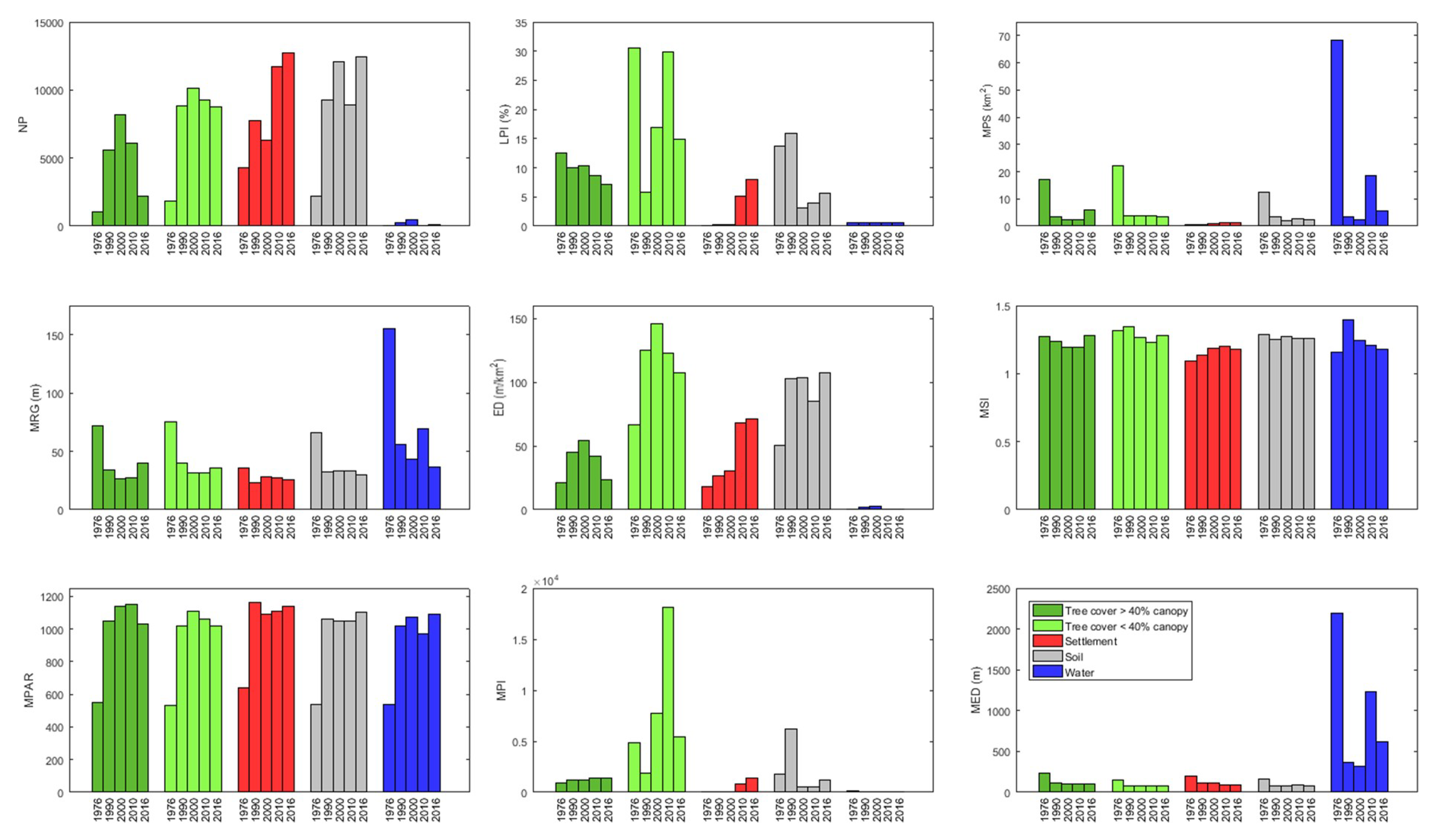
The results of landscape analysis in this study reveal that the ICT urban landscape has become more heterogeneous, disproportional and diverse, and tree patches have declined. Alarmingly, core forests of >500 acres have declined almost 15% in forty years. Although at the individual level, the residents of ICT, civil society, and the local government are trying to recover tree cover loss by planting trees, but these initiatives should be continuous and ongoing on a regular basis to monitor the growth of trees without damaging the existing mature standing trees. The temporal forest fragmentation analysis shows that due to tree cover loss, the three categories of core forest fragmentations (i.e., <250 acres, 250–500 acres, and >500 acres) have decreased in forty years (1976–2016). The loss in forest fragmentation negatively influences the habitat and terrestrial biodiversity of ICT [79,90,91]. Based on landscape metrics analysis over the Dhaka metropolitan, a similar Asian developing city, Dewan et al. [31] revealed that cultivated areas and vegetated lands became highly fragmented with increasing anthropogenic disturbances and urban built up category became aggregated and convoluted.
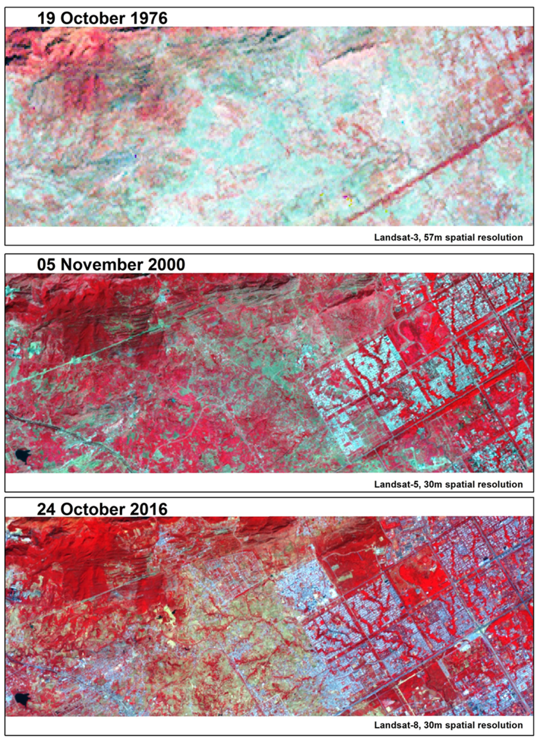
While our analysis of ICT land cover change dynamics in this study is important and unique, there are a few caveats which are worth mentioning. First of all, for the 1976 land cover map, we have relied on approximately 57 m spatial resolution Landsat 3 Multispectral Scanner System (MSS) sensor data which is relatively coarser spatially as compared to Landsat 5 and 8 (i.e., 30 m), which may affect the spatial heterogeneity and accuracy of developed land cover maps. Second, as Landsat is a pioneer Earth Observation (EO) satellite program initiated in 1972, so acquiring remote sensing imagery of the years before that is not possible, and thus we cannot derive land cover maps before the 1960s, when the Islamic Republic of Pakistan’s capital shifted from Karachi to Islamabad. Third, from Landsat 30 m medium spatial resolution satellite data, we cannot detect and delineate the boundaries of built-up areas as well as can be done from sub-meter VHRS images available from the 2000s onward. However, the VHRS datasets come with a high cost, especially when acquisitions at multiples times have to be acquired, and may not be therefore feasible for study sites in developing countries. Of course, research in this domain is ongoing with regards to utilization of VHRS data for study of urban areas, using methods like object-based image analysis, machine learning, etc. Fourth, there may be some level of uncertainty for the field measurement data, as there is always a potential for human error especially when ground truth is collected over larger areas. Fifth, in this study, we utilized only temporal optical satellite data, which may cause optical signal saturation in closed canopy forests, and atmospheric effects (i.e., cloud coverage, haze, and smog).

6. Conclusions

This study sheds new light on systematic land cover dynamics of ICT over the period of four decades, underlining a major decrease in tree cover along with significant increase in settlements and soil. The findings from the analysis of land cover changes, landscape metrics, forest fragmentation, and LCRPGR, are aligned well and agree overall with previous published work on the regional and global scales. The computation of LCRPGR is vital to understand the rate of land change as compared to the population boom, to understand historical land consumption traditions, and to guide decision and policy makers on planned urban expansion while ensuring the protection of environmental, social, and economic assets. It is indeed a scientifically accepted phenomenon that in most of the cities, the land consumption rate overall is much faster than the population growth rate, due to high demand of luxurious occupancies in the urban areas.
Both natural and anthropogenic activities are responsible for land cover changes in ICT. In terms of landscape and fragmentations, the ICT urban landscape ecology is continuously under threat due to the encroachment of housing societies, and influential business community. The findings from urban landscape matrix and forest fragmentation analysis in this study could help ICT Capital Development Authority (CDA) and Islamabad Wildlife Management Board (IWMB) in making strategic decisions to prevent tree loss, forest degradation, and encroachment in the urban landscape of ICT, and also plan future urban growth keeping with the use of remote sensing imagery and geospatial analysis. The methodology outlined in this study is cost-effective and could be easily replicable to other countries/regions, especially in developing countries, through integrating freely available satellite images with a 5–10 years interval.

Author Contributions

Conceptualization, H.G., W.A.Q.; data analysis, S.A., M.K.; supervision, H.G., visualization, H.G., W.A.Q., S.A., M.K.; writing—original draft preparation, H.G., S.A., W.A.Q., S.M.A.; writing—review and editing, H.G., W.A.Q., S.M.A. All authors have read and approved the final version of this paper. All authors have read and agreed to the published version of the manuscript.

Funding

This research received no external funding.

Acknowledgments

This work is an extension of an Undergraduate Final Year Project, which was completed in 2018, and we would like to express our thanks to Institute of Space Technology (IST) management and academic staff for their support. The authors also would like to acknowledge the editors and three anonymous reviewers for their extensive and critical comments on the paper, which helped to improve the paper immensely.

Conflicts of Interest

The authors declare no conflict of interest. The views and interpretations in this publication are those of the authors, and they are not necessarily attributable to their organizations.

Appendix A

Table A1. Accuracy assessment of land covers classification for 1976, 1990, 2000, 2010, and 2016.
2016’s Land cover accuracy assessment report
Tree cover > 40% canopyTree cover < 40% canopySettlementSoilWaterTotalUser’s accuracy (%)
Tree cover >40% canopy2230002588
Tree cover <40% canopy3210102584
Settlement0023302688
Soil0122102488
Water00002525100
Total2525252525125
Producer’s accuracy (%)88849284100
Overall accuracy: 0.90, Kappa: 0.85
2010’s Land cover accuracy assessment report
Tree cover >40% canopy2250012879
Tree cover <40% canopy3200002387
Settlement0023402785
Soil0022102391
Water00002424100
Total2525252525
Producer’s accuracy (%)8880928496
Overall accuracy: 0.88, Kappa: 0.84
2000’s Land cover accuracy assessment report
Tree cover >40% canopy2230022781
Tree cover <40% canopy3201102580
Settlement0022302588
Soil0222102584
Water00002323100
Total2525252525125
Producer’s accuracy (%)8880888492
Overall accuracy: 0.86, Kappa: 0.82
1990’s Land cover accuracy assessment report
Tree cover >40% canopy2120012488
Tree cover <40% canopy4201102677
Settlement0021402584
Soil0332002677
Water00002424100
Total2525252525125
Producer’s accuracy (%)8480848096
Overall accuracy: 0.85, Kappa: 0.81
1976’s Land cover accuracy assessment report
Tree cover >40% canopy2130012584
Tree cover <40% canopy4211202875
Settlement0020502580
Soil0141802378
Water00002424100
Total2525252525125
Producer’s accuracy (%)8484807296
Overall accuracy: 0.83, Kappa: 0.79
Table A2. Land cover class level landscape matrix parameters results for 1976, 1990, 2000, 2010, and 2016.
Land Cover ClassYearPatch Density and SizeShape and EdgeProximity/Isolation
NPLPI (%)MPS (km2)MRG (m)ED (m/km2)MSIMPAR ×103MPIMED (m)
Tree cover >40% canopy1976107212.5016.9871.5821.081.270.55869.65228.47
199055909.953.4434.1344.781.241.051233.12109.63
2000819510.312.1826.8954.251.191.141247.7798.59
201061218.592.3027.3441.941.201.151401.38104.15
201622237.105.9540.3023.541.281.031407.0399.17
Tree cover <40% canopy1976187230.6222.2975.5266.351.320.534809.76145.76
199088565.893.8740.00125.301.351.021837.1977.20
20001014516.923.9431.18146.141.261.117773.8173.00
2010925329.833.8931.39122.421.231.0618114.3279.52
2016872814.973.5136.00107.081.281.025386.7083.08
Settlement197642960.020.7035.8317.731.090.641.06193.66
199077520.220.5722.9226.691.131.1612.70116.02
200063100.300.9528.2830.581.191.0933.80115.14
2010116945.161.2327.3968.281.201.11784.8686.70
2016127548.071.3425.5671.351.181.141382.8187.29
Soil1976218013.7612.4065.8650.431.290.541763.86159.37
1990927115.943.4232.34102.901.251.066172.9781.38
2000120603.152.1333.12103.571.271.05564.4780.48
201088854.022.8633.4984.811.261.05530.0585.99
2016124365.722.3330.23107.681.261.11197.4276.53
Water197680.6068.27154.900.251.150.54162.662192.65
19902420.623.4955.791.901.391.0229.98362.05
20004490.612.3543.542.931.251.0726.36322.78
2010340.5918.5169.640.471.210.9765.201230.49
20161200.585.4336.360.711.181.0946.78620.00
Table A3. Forest fragmentation results for 1976, 1990, 2000, 2010, and 2016 and percentage assessment based on satellite images).
Forest Fragmentation Classes19761990200020102016
km2
Patch14.74 (2.46)15.67 (2.93)15.46 (2.68)17.84 (3.56)19.92 (4.54)
Edge105.58 (17.62)119.48 (22.33)123.42 (21.36)94.06 (18.75)96.83 (22.07)
Perforated35.21 (5.88)31.52 (5.89)41.79 (7.23)24.39 (4.86)22.74 (5.18)
Core (<250 acres)41.4 (6.91)79.94 (14.94)68.04 (11.77)52.05 (10.38)52.24 (11.91)
Core (250–500 acres)10.99 (1.83)17.18 (3.21)15.74 (2.72)5.54 (1.10)5.63 (1.28)
Core (>500 acres)391.98 (65.41)271.34 (50.71)313.42 (54.24)307.67 (61.34)241.44 (55.02)
Total585.16 (100)535.13 (100)577.87 (100)501.55 (100)438.80 (100)

References

  1. Lambin, E.F.; Meyfroidt, P. Land use transitions: Socio-ecological feedback versus socio-economic change. Land Use Policy 2010, 27, 108–118. [Google Scholar] [CrossRef]
  2. Balooni, K.; Lund, J.F. Forest rights: The hard currency of REDD+. Conserv. Lett. 2014, 7, 278–284. [Google Scholar] [CrossRef] [Green Version]
  3. Belal, A.A.; Moghanm, F.S. Detecting urban growth using remote sensing and GIS techniques in Al Gharbiya governorate, Egypt. Egypt. J. Remote Sens. Sp. Sci. 2011, 14, 73–79. [Google Scholar] [CrossRef] [Green Version]
  4. Congalton, R.; Gu, J.; Yadav, K.; Thenkabail, P.; Ozdogan, M. Global Land Cover Mapping: A Review and Uncertainty Analysis. Remote Sens. 2014, 6, 12070–12093. [Google Scholar] [CrossRef] [Green Version]
  5. Rasul, G. Ecosystem services and agricultural land-use practices: A case study of the Chittagong Hill Tracts of Bangladesh. Sustain. Sci. Pract. Policy 2009, 5, 15–27. [Google Scholar] [CrossRef]
  6. Addae, B.; Oppelt, N. Land-Use/Land-Cover Change Analysis and Urban Growth Modelling in the Greater Accra Metropolitan Area (GAMA), Ghana. Urban Sci. 2019, 3, 26. [Google Scholar] [CrossRef] [Green Version]
  7. Redman, C.L. Human Dimensions of Ecosystem Studies. Ecosystems 1999, 2, 296–298. [Google Scholar] [CrossRef]
  8. Xu, C.; Liu, M.; Zhang, C.; An, S.; Yu, W.; Chen, J.M. The spatiotemporal dynamics of rapid urban growth in the Nanjing metropolitan region of China. Landsc. Ecol. 2007, 22, 925–937. [Google Scholar] [CrossRef]
  9. Burgi, M.; Hersperger, A.M.; Schneeberger, N. Driving forces of landscape change - current and new directions. Landsc. Ecol. 2005, 19, 857–868. [Google Scholar] [CrossRef]
  10. Bilsborrow, R.E.; McDevitt, T.M.; Kossoudji, S.; Fuller, R. The Impact of Origin Community Characteristics on Rural-Urban Out-Migration in a Developing Country. Demography 1987, 24, 191–210. [Google Scholar] [CrossRef]
  11. Magidi, J.; Ahmed, F. Assessing urban sprawl using remote sensing and landscape metrics: A case study of City of Tshwane, South Africa (1984–2015). Egypt. J. Remote Sens. Sp. Sci. 2019, 22, 335–346. [Google Scholar] [CrossRef]
  12. Melchiorri, M.; Pesaresi, M.; Florczyk, A.J.; Corbane, C.; Kemper, T. Principles and applications of the global human settlement layer as baseline for the land use efficiency indicator—SDG 11.3.1. ISPRS Int. J. Geo-Inf. 2019, 8, 96. [Google Scholar] [CrossRef] [Green Version]
  13. Sharma, L.; Pandey, P.C.; Nathawat, M.S. Assessment of land consumption rate with urban dynamics change using geospatial techniques. J. Land Use Sci. 2012, 7, 135–148. [Google Scholar] [CrossRef]
  14. Salvati, L.; Carlucci, M. Distance matters: Land consumption and the mono-centric model in two southern European cities. Landsc. Urban Plan. 2014, 127, 41–51. [Google Scholar] [CrossRef]
  15. Sibly, R.M.; Hone, J. Population growth rate and its determinants: An overview. Philos. Trans. R. Soc. B Biol. Sci. 2002, 357, 1153–1170. [Google Scholar] [CrossRef]
  16. Philippe, D.; Jean-Marie, O.-B.; Marta, G.-D.; Thomas, C. Global immunization: Status, progress, challenges and future. BMC Int. Health Hum. Rights 2009, 9, S2. [Google Scholar] [CrossRef] [Green Version]
  17. Ghazanfari, H.; Namiranian, M.; Sobhani, H.; Mohajer, R.M. Traditional forest management and its application to encourage public participation for sustainable forest management in the northern Zagros mountains of Kurdistan Province, Iran. Scand. J. For. Res. Suppl. 2004, 19, 65–71. [Google Scholar] [CrossRef]
  18. Turner, A.B.L.; Meyer, W.B.; Skole, D.L. Global land-use/land-cover change: Towards an integrated study. Ambio 1994, 23, 91–95. [Google Scholar]
  19. Seto, K.C.; Guneralp, B.; Hutyra, L.R. Global forecasts of urban expansion to 2030 and direct impacts on biodiversity and carbon pools. Proc. Natl. Acad. Sci. 2012, 109, 16083–16088. [Google Scholar] [CrossRef] [PubMed] [Green Version]
  20. Grimm, N.B.; Faeth, S.H.; Golubiewski, N.E.; Redman, C.L.; Wu, J.; Bai, X.; Briggs, J.M. Global Change and the Ecology of Cities. Science. 2008, 319, 756–760. [Google Scholar] [CrossRef] [PubMed] [Green Version]
  21. Angel, S.; Parent, J.; Civco, D.L.; Blei, A.; Potere, D. The dimensions of global urban expansion: Estimates and projections for all countries, 2000–2050. Prog. Plann. 2011, 75, 53–107. [Google Scholar] [CrossRef]
  22. Boggs, G.S. Assessment of SPOT 5 and QuickBird remotely sensed imagery for mapping tree cover in savannas. Int. J. Appl. Earth Obs. Geoinf. 2010, 12, 217–224. [Google Scholar] [CrossRef]
  23. Wulder, M.A.; Coops, N.C.; Roy, D.P.; White, J.C.; Hermosilla, T. Land cover 2.0. Int. J. Remote Sens. 2018, 39, 4254–4284. [Google Scholar] [CrossRef] [Green Version]
  24. Dong, J.; Xiao, X.; Menarguez, M.A.; Zhang, G.; Qin, Y.; Thau, D.; Biradar, C.; Moore, B. Mapping paddy rice planting area in northeastern Asia with Landsat 8 images, phenology-based algorithm and Google Earth Engine. Remote Sens. Environ. 2016, 185, 142–154. [Google Scholar] [CrossRef] [Green Version]
  25. Uddin, K.; Shrestha, H.L.H.L.; Murthy, M.S.R.S.R.; Bajracharya, B.; Shrestha, B.; Gilani, H.; Pradhan, S.; Dangol, B. Development of 2010 national land cover database for the Nepal. J. Environ. Manage. 2015, 148, 82–90. [Google Scholar] [CrossRef]
  26. Seto, K.C.; Fragkias, M.; Güneralp, B.; Reilly, M.K. A Meta-Analysis of Global Urban Land Expansion. PLoS ONE 2011, 6, e23777. [Google Scholar] [CrossRef]
  27. Yang, C.; Li, Q.; Hu, Z.; Chen, J.; Shi, T.; Ding, K.; Wu, G. Spatiotemporal evolution of urban agglomerations in four major bay areas of US, China and Japan from 1987 to 2017: Evidence from remote sensing images. Sci. Total Environ. 2019, 671, 232–247. [Google Scholar] [CrossRef]
  28. Herold, M.; Couclelis, H.; Clarke, K.C. The role of spatial metrics in the analysis and modeling of urban land use change. Comput. Environ. Urban Syst. 2005, 29, 369–399. [Google Scholar] [CrossRef]
  29. Gong, C.; Yu, S.; Joesting, H.; Chen, J. Determining socioeconomic drivers of urban forest fragmentation with historical remote sensing images. Landsc. Urban Plan. 2013, 117, 57–65. [Google Scholar] [CrossRef]
  30. Huang, J.; Lu, X.X.; Sellers, J.M. A global comparative analysis of urban form: Applying spatial metrics and remote sensing. Landsc. Urban Plan. 2007, 82, 184–197. [Google Scholar] [CrossRef]
  31. Dewan, A.M.; Yamaguchi, Y.; Ziaur Rahman, M. Dynamics of land use/cover changes and the analysis of landscape fragmentation in Dhaka Metropolitan, Bangladesh. GeoJournal 2012, 77, 315–330. [Google Scholar] [CrossRef]
  32. Mandelas, E. A fuzzy cellular automata based shell for modeling urban growth–a pilot application in Mesogia area. In Proceedings of the 10th AGILE International Conference on Geographic Information Science, Allborg, Denmark, 8–11 May 2007; pp. 1–9. [Google Scholar]
  33. Farhat, K.; Waseem, L.A.; Khan, A.A.; Baig, S. Spatiotemporal Demographic Trends and Land Use Dynamics of Metropolitan Lahore. J. Hist. Cult. Art Res. 2018, 7, 92. [Google Scholar] [CrossRef] [Green Version]
  34. Shah, M.H.; Shaheen, N. Seasonal behaviours in elemental composition of atmospheric aerosols collected in Islamabad, Pakistan. Atmos. Res. 2010, 95, 210–223. [Google Scholar] [CrossRef]
  35. Butt, M.J.; Waqas, A.; Iqbal, M.F.; Muhammad, G.; Lodhi, M.A.K. Assessment of Urban Sprawl of Islamabad Metropolitan Area Using Multi-Sensor and Multi-Temporal Satellite Data. Arab. J. Sci. Eng. 2012, 37, 101–114. [Google Scholar] [CrossRef]
  36. Shahzad, N.; Saeed, U.; Gilani, H.; Ahmad, S.R.; Ashraf, I.; Irteza, S.M. Evaluation of state and community/private forests in Punjab, Pakistan using geospatial data and related techniques. For. Ecosyst. 2015, 2, 7. [Google Scholar] [CrossRef] [Green Version]
  37. Doxiadis, C.A. Islamabad, the creation of a new capital. Town Plan. Rev. 1965, 36, 1. [Google Scholar] [CrossRef] [Green Version]
  38. Stephenson, G.V. Two Newly Created Capitals: Islamabad and Brasilia. Town Plan. Rev. 1970, 41, 317. [Google Scholar] [CrossRef]
  39. Kreutzmann, H. Islamabad, living the plan. Südasien-Chronik-South Asia Chron. 2013, 3, 2013. [Google Scholar]
  40. Beacco, D. Urban Planning in Islamabad: From the Modern Movement to the Contemporary Urban Development Between Formal and Informal Settlements. In Sustainable Urban Development and Globalization; Springer: Cham, Switzerland, 2018; pp. 65–74. [Google Scholar]
  41. Bokhari, S.A.; Saqib, Z.; Ali, A.; Haq, M.Z. Perception of Residents about Urban Vegetation: A Comparative Study of Planned Versus Semi-Planned Cities of Islamabad and Rawalpindi, Pakistan. J. Ecosyst. Ecography 2018, 8, 1–8. [Google Scholar] [CrossRef]
  42. Naeem, S.; Cao, C.; Waqar, M.M.; Wei, C.; Acharya, B.K. Vegetation role in controlling the ecoenvironmental conditions for sustainable urban environments: A comparison of Beijing and Islamabad. J. Appl. Remote Sens. 2018, 12, 016013. [Google Scholar] [CrossRef] [Green Version]
  43. Adeel, M. Methodology for identifying urban growth potential using land use and population data: A case study of Islamabad Zone IV. Procedia Environ. Sci. 2010, 2, 32–41. [Google Scholar] [CrossRef] [Green Version]
  44. Butt, A.; Shabbir, R.; Ahmad, S.S.; Aziz, N. Land use change mapping and analysis using Remote Sensing and GIS: A case study of Simly watershed, Islamabad, Pakistan. Egypt. J. Remote Sens. Sp. Sci. 2015, 18, 251–259. [Google Scholar] [CrossRef] [Green Version]
  45. Butt, A.; Shabbir, R.; Ahmad, S.S.; Aziz, N.; Nawaz, M.; Shah, M.T.A. Land cover classification and change detection analysis of Rawal watershed using remote sensing data. J Biodivers Env. Sci 2015, 6, 236–248. [Google Scholar]
  46. Hassan, Z.; Shabbir, R.; Ahmad, S.S.; Malik, A.H.; Aziz, N.; Butt, A.; Erum, S. Dynamics of land use and land cover change (LULCC) using geospatial techniques: A case study of Islamabad Pakistan. Springerplus 2016, 5, 812. [Google Scholar] [CrossRef] [PubMed] [Green Version]
  47. Sohail, M.T.; Mahfooz, Y.; Azam, K.; Yat, Y.; Genfu, L.; Fahad, S. Impacts of urbanization and land cover dynamics on underground water in Islamabad, Pakistan. Desalin. WATER Treat. 2019, 159, 402–411. [Google Scholar] [CrossRef]
  48. Naeem, S.; Cao, C.; Qazi, W.; Zamani, M.; Wei, C.; Acharya, B.; Rehman, A. Studying the association between green space characteristics and land surface temperature for sustainable urban environments: An analysis of Beijing and Islamabad. ISPRS Int. J. Geo-Inf. 2018, 7, 38. [Google Scholar] [CrossRef] [Green Version]
  49. Khalid, N.; Ullah, S.; Ahmad, S.S.; Ali, A.; Chishtie, F. A remotely sensed tracking of forest cover and associated temperature change in Margalla hills. Int. J. Digit. Earth 2019, 12, 1133–1150. [Google Scholar] [CrossRef]
  50. Batool, R.; Javaid, K. Spatio-temporal assessment of Margalla hills forest by using Landsat imagery for year 2000 and 2018. In Proceedings of the International Archives of the Photogrammetry, Remote Sensing and Spatial Information Sciences, ISPRS TC III Mid-term Symposium “Developments, Technologies and Applications in Remote Sensing”, Beijing, China, 7–10 May 2018; Volume XLII–3, pp. 69–72. [Google Scholar]
  51. Mannan, A.; Liu, J.; Zhongke, F.; Khan, T.U.; Mukete, B.; Chaoyong, S.; Saeed, S.; Yongxiang, F.; Ahmad, A.; Amir, M.; et al. Application of land-use/land cover changes in monitoring and projecting forest biomass carbon loss in Pakistan. Glob. Ecol. Conserv. 2019, 17, e00535. [Google Scholar] [CrossRef]
  52. Dewan, A.M.; Yamaguchi, Y. Land use and land cover change in Greater Dhaka, Bangladesh: Using remote sensing to promote sustainable urbanization. Appl. Geogr. 2009, 29, 390–401. [Google Scholar] [CrossRef]
  53. Dewan, A.M.; Yamaguchi, Y. Using remote sensing and GIS to detect and monitor land use and land cover change in Dhaka Metropolitan of Bangladesh during 1960–2005. Environ. Monit. Assess. 2009, 150, 237–249. [Google Scholar] [CrossRef]
  54. Pramanik, M.M.A.; Stathakis, D. Forecasting urban sprawl in Dhaka city of Bangladesh. Environ. Plan. B Plan. Des. 2016, 43, 756–771. [Google Scholar] [CrossRef] [Green Version]
  55. Gruebner, O.; Sachs, J.; Nockert, A.; Frings, M.; Khan, M.M.H.; Lakes, T.; Hostert, P. Mapping the Slums of Dhaka from 2006 to 2010. Dataset Pap. Sci. 2014, 2014, 1–7. [Google Scholar] [CrossRef] [Green Version]
  56. Sharma, R.; Joshi, P.K. Monitoring Urban Landscape Dynamics Over Delhi (India) Using Remote Sensing (1998–2011) Inputs. J. Indian Soc. Remote Sens. 2013, 41, 641–650. [Google Scholar] [CrossRef]
  57. Naeem, S.; Cao, C.; Fatima, K.; Najmuddin, O.; Acharya, B.K. Landscape greening policies-based land use/land cover simulation for Beijing and Islamabad—An implication of sustainable urban ecosystems. Sustainability 2018, 10, 1049. [Google Scholar] [CrossRef] [Green Version]
  58. Huang, H.; Chen, Y.; Clinton, N.; Wang, J.; Wang, X.; Liu, C.; Gong, P.; Yang, J.; Bai, Y.; Zheng, Y.; et al. Mapping major land cover dynamics in Beijing using all Landsat images in Google Earth Engine. Remote Sens. Environ. 2017, 202, 166–176. [Google Scholar] [CrossRef]
  59. Cui, L.; Shi, J. Urbanization and its environmental effects in Shanghai, China. Urban Clim. 2012, 2, 1–15. [Google Scholar] [CrossRef] [Green Version]
  60. Zhao, S.; Da, L.; Tang, Z.; Fang, H.; Song, K.; Fang, J. Ecological consequences of rapid urban expansion: Shanghai, China. Front. Ecol. Environ. 2006, 4, 341–346. [Google Scholar]
  61. Yue, W.; Fan, P.; Wei, Y.D.; Qi, J. Economic development, urban expansion, and sustainable development in Shanghai. Stoch. Environ. Res. Risk Assess. 2014, 28, 783–799. [Google Scholar] [CrossRef]
  62. Bagan, H.; Yamagata, Y. Landsat analysis of urban growth: How Tokyo became the world’s largest megacity during the last 40 years. Remote Sens. Environ. 2012, 127, 210–222. [Google Scholar] [CrossRef]
  63. Sheikh, I.M.; Pasha, M.K.; Williams, V.S.; Raza, S.Q.; Khan, K.S.A.A. Environmental Geology of the Islamabad-Rawalpindi Area. In Regional Studies of the Potwar Plateau Area, Northern Pakistan; 2007; pp. 1–32. Available online: https://pubs.usgs.gov/bul/2078/ (accessed on 5 February 2020).
  64. Teillet, P.; Barker, J.; Markham, B.; Irish, R.; Fedosejevs, G.; Storey, J. Radiometric cross-calibration of the Landsat-7 ETM+ and Landsat-5 TM sensors based on tandem data sets. Remote Sens. Environ. 2001, 78, 39–54. [Google Scholar] [CrossRef] [Green Version]
  65. Tan, B.; Masek, J.G.; Wolfe, R.; Gao, F.; Huang, C.; Vermote, E.F.; Sexton, J.O.; Ederer, G. Improved forest change detection with terrain illumination corrected Landsat images. Remote Sens. Environ. 2013, 136, 469–483. [Google Scholar] [CrossRef]
  66. Congalton, R.G. Remote Sensing and Image Interpretation. 7th Edition. Photogramm. Eng. Remote Sens. 2015, 81, 615–616. [Google Scholar] [CrossRef]
  67. Kasereka, K. Remote Sensing and Geographic Information System for Inferring Land Cover and Land Use Change in Wuhan (China), 1987-2006. J. Sustain. Dev. 2010, 3, 221–229. [Google Scholar] [CrossRef] [Green Version]
  68. Khatami, R.; Mountrakis, G.; Stehman, S.V. A meta-analysis of remote sensing research on supervised pixel-based land-cover image classification processes: General guidelines for practitioners and future research. Remote Sens. Environ. 2016, 177, 89–100. [Google Scholar] [CrossRef] [Green Version]
  69. Saura, S. Effects of minimum mapping unit on land cover data spatial configuration and composition. Int. J. Remote Sens. 2002, 23, 4853–4880. [Google Scholar] [CrossRef]
  70. Roy, P.S.; Roy, A.; Joshi, P.K.; Kale, M.P.; Srivastava, V.K.; Srivastava, S.K.; Dwevidi, R.S.; Joshi, C.; Behera, M.D.; Meiyappan, P.; et al. Development of decadal (1985-1995-2005) land use and land cover database for India. Remote Sens. 2015, 7, 2401–2430. [Google Scholar] [CrossRef] [Green Version]
  71. Rosenfield, G.H.; Fitzpatrick-Lins, K. A coefficient of agreement as a measure of thematic classification accuracy. Photogramm. Eng. Remote Sens. 1986, 52, 223–227. [Google Scholar]
  72. Puyravaud, J.P. Standardizing the calculation of the annual rate of deforestation. For. Ecol. Manage. 2003, 177, 593–596. [Google Scholar] [CrossRef]
  73. McGarigal, K. Landscape Pattern Metrics. In Wiley StatsRef: Statistics Reference Online; John Wiley & Sons, Ltd.: Chichester, UK, 2014; Volume 45, pp. 1–18. [Google Scholar]
  74. Nichol, J.E.; Abbas, S.; Fischer, G.A. Spatial patterns of degraded tropical forest and biodiversity restoration over 70-years of succession. Glob. Ecol. Conserv. 2017, 11, 134–145. [Google Scholar] [CrossRef]
  75. McGarigal, K.; Marks, B.J. FRAGSTATS: Spatial pattern analysis program for quantifying landscapes structure. Gen. Tech. Rep. PNW-GTR-351. U.S. Dep. Agric. For. Serv. Pacific Northwest Res. Station. Portland, OR 1994, 97331, 134. [Google Scholar]
  76. Vogt, P.; Riitters, K.; Estreguil, C.; Kozak, J.; Wade, T.; Wickham, J. Mapping spatial patterns with morphological image processing. Landsc. Ecol. 2007, 22, 171–177. [Google Scholar] [CrossRef]
  77. Nicolau, R.; Caetano, M.; David, J.; Caetano, M.; Pereira, J. Ratio of Land Consumption Rate to Population Growth Rate—Analysis of Different Formulations Applied to Mainland Portugal. ISPRS Int. J. Geo-Inf. 2018, 8, 10. [Google Scholar] [CrossRef] [Green Version]
  78. Khalid, N.; Saeed Ahmad, S. Monitoring Forest cover change of Margalla Hills over a period of two decades (1992-2011): A spatiotemporal perspective. J. Ecosyst. Ecography 2016, 06, 1–8. [Google Scholar] [CrossRef]
  79. Malik, I.U.; Faiz, A.H.; -i- Abbas, F. Biodiversity Assessment and its Effect on the Environment of Shakarparian Forest. J. Bioresour. Manag. 2014, 1, 4. [Google Scholar] [CrossRef] [Green Version]
  80. Ahmed, K.; Jatoo, W.; Jing, F.C.; Saengkrod, W.; Mastoi, A.G. Urbanization in Pakistan: Challenges and Way Forward (Options) For Sustainable Urban Development. In Proceedings of the 4th International Conference on Energy, Environment and Sustainable Development, Jamshoro, Pakistan, 1–3 November 2016. [Google Scholar]
  81. Wang, Y.; Huang, C.; Feng, Y.; Zhao, M.; Gu, J. Using Earth Observation for Monitoring SDG 11.3.1- Ratio of Land Consumption Rate to Population Growth Rate in Mainland China. Remote Sens. 2020, 12, 357. [Google Scholar] [CrossRef] [Green Version]
  82. Rimal, B. Application of remote sensing and GIS, land use/land cover change in Kathmandu Metropolitan City, Nepal. J. Theor. Appl. Inf. Technol. 2011, 23, 80–86. [Google Scholar]
  83. Thapa, B.R.; Ishidaira, H.; Pandey, V.P.; Shakya, N.M. A multi-model approach for analyzing water balance dynamics in Kathmandu Valley, Nepal. J. Hydrol. Reg. Stud. 2017, 9, 149–162. [Google Scholar] [CrossRef]
  84. Giri, N.; Singh, O.P. Urban growth and water quality in Thimphu, Bhutan. J. Urban Environ. Eng. 2013, 7, 82–95. [Google Scholar] [CrossRef]
  85. Khanal, N.; Uddin, K.; Matin, M.; Tenneson, K. Automatic Detection of Spatiotemporal Urban Expansion Patterns by Fusing OSM and Landsat Data in Kathmandu. Remote Sens. 2019, 11, 2296. [Google Scholar] [CrossRef] [Green Version]
  86. Ellis, S.; Taylor, D.; Masood, K.R. Land degradation in northern Pakistan. Geography 1993, 78, 84–87. [Google Scholar]
  87. Cavanaugh, R. Increased pollution and problems in respiratory health menace Pakistan’s soaring population. Lancet Respir. Med. 2018, 6, 175–176. [Google Scholar] [CrossRef]
  88. Rashid, K.; Rasul, G. Rainfall variability and maize production over the Potohar plateau of Pakistan. Pakistan J. Meteorol. 2011, 8, 63–74. [Google Scholar]
  89. Pandey, V.P.; Manandhar, S.; Kazama, F. Climate change vulnerability assessment. In Climate Change and Water Resources; CRC Press: Boca Raton, FL, USA, 2014; pp. 183–208. ISBN 9781466594678. [Google Scholar]
  90. Akram, A.; Rais, M.; Asadi, M.A.; Jilani, M.J.; Balouch, S.; Anwar, M.; Saleem, A. Do habitat variables correlate anuran abundance in arid terrain of Rawalpindi–Islamabad Areas, Pakistan? J. King Saud Univ. Sci. 2015, 27, 278–283. [Google Scholar] [CrossRef] [Green Version]
  91. Shabbir, A.; Bajwa, R. Distribution of parthenium weed (Parthenium hysterophorus L.), an alien invasive weed species threatening the biodiversity of Islamabad. Weed Biol. Manag. 2006, 6, 89–95. [Google Scholar] [CrossRef]
Figure 1. Study area map—Islamabad Capital Territory (ICT), Pakistan. The bounded box inset covering Zone I and Zone II partially is representing the area shown in the Figure in Section 5.
Land 09 00123 g001
Figure 2. Methodological flow chart.
Land 09 00123 g002
Figure 3. Land cover maps for 1976, 1990, 2000, 2010, and 2016.
Land 09 00123 g003
Figure 4. Land cover class level landscape matrix parameters graphs for 1976, 1990, 2000, 2010, and 2016.
Land 09 00123 g004
Figure 5. Forest fragmentation maps for 1976, 1990, 2000, 2010, and 2016.
Land 09 00123 g005
Figure 6. Forest fragmentation graphs for 1976, 1990, 2000, 2010, and 2016.
Land 09 00123 g006
Figure 7. Temporal Landsat satellite images of 1976, 2000, and 2016 in standard False Color Composite (FCC), illustrating an overall increase in built-up areas over the years in the ICT. The area of the ICT shown here represents the bounded box inset covering Zone I and Zone II partially in Figure 1.
Land 09 00123 g007
Table 1. Landsat images used for land cover mapping.
Acquisition DateSatelliteSensorPath/RowSpatial Resolution
19 October 1976Landsat 3MSS161/3757 m
01 October 1990Landsat 5TM150/3730 m
05 November 2000Landsat 7ETM+150/3730 m
09 November 2010Landsat 5TM150/3730 m
24 October 2016Landsat 8OLI150/3730 m
Table 2. Population data of ICT for 1972, 1976, 1998/2000, and 2016/2017.
Year197219761998/20002016/2017
Population238,000 291,888 805,235 2,006,572
Table 3. Land cover class level description of landscape metrics used in this study.
CategoryMetricsUnitDescription
Patch size and densityNumber of Patches (NP) Gives the total number of patches in the landscape of a particular category.
Largest Patch Index (LPI)Percentage (%)Ratio of area of largest patch to total landscape area.
Mean Patch Size (MPS)Square Kilometer (km2)Sum of area of all the patches divided by the number of patches of the class.
Mean Radius of Gyration (MRG)Meter (m)Mean distance for each cell in one patch to the patch centroid. It measures connectivity inside habitat patches.
Shape and edgeEdge Density (ED)Meter per Square Kilometer (m/km2)Measures total length of edge per unit area. It explains complexity of patch shape.
Mean Shape Index (MSI) Measures complexity of patch shape compared to a standard shape of the same size. Its value increases with complexity of shape.
Mean Perimeter to Area Ratio (MPAR) Patch shape complexity, based on perimeter length to patch area. It explains shape complexity without standardization to a standard Euclidean shape (square).
Proximity/IsolationMean Proximity Index (MPI) Measure of connectedness of a habitat class. Considers size and proximity of all patches with the same habitat type inside a specified search radius.
Mean Euclidean Nearest Neighbor Distance (MED)Meter (m)Measures minimum edge-to-edge distance to the nearest neighboring patch of the same type. It explains connectedness or isolation in landscape or habitat class.
Table 4. Land cover 1976, 1990, 2000, 2010, and 2016 assessment based on satellite images.
Land Cover Classes19761990200020102016
km2 (%)
Tree cover >40% canopy182.87 (20.18)192.19 (21.21)178.56 (19.70)140.76 (15.53)132.27 (10.86)
Tree cover <40% canopy417.03 (46.02)342.94 (37.85)399.31 (44.07)360.79 (39.82)306.53 (35.72)
Settlement29.99 (3.31)44.51 (4.91) 59.73 (6.60) 143.82 (15.87) 170.40 (18.80)
Soil270.27 (29.83) 317.91 (35.08)257.00 (28.37)254.34 (28.02) 289.45 (33.82)
Water5.86 (0.65)8.44 (0.94)10.51 (1.16)6.29 (0.69)6.51 (0.76)
Total906 (100)
Table 5. Land cover annual rate of change (% change per year) from 1976–1990, 1990–2000, 2000–2010, 2010–2016, and 1976–2016.
Land Cover Classes1976–19901990–20002000–20102010–20161976–2016
Tree cover >40% canopy0.36−0.74−2.38−1.04−0.81
Tree cover <40% canopy−1.401.52−1.01−2.72−0.77
Settlements2.822.948.792.834.34
Soil1.16−2.09−0.142.160.17
Water2.612.19−5.131.590.42

