Trade-Offs between Economic Benefits and Ecosystem Services Value under Three Cropland Protection Scenarios for Wuhan City in China

Abstract

Over the past few decades urbanization and population growth have been the main trend all over the world, which brings the increase of economic benefits (EB) and the decrease of cropland. Cropland protection policies play an important role in the urbanization progress. In this study, we assess the trade-offs between EB and ecosystem services value (ESV) under three cropland protection policy scenarios using the LAND System Cellular Automata for Potential Effects (LANDSCAPE) model. The empirical results reveal that trade-offs between EB and ESV in urbanizing areas are dynamic, and that they considerably vary under different cropland protection policy scenarios. Especially, the results identify certain “turning points” for each policy scenario at which a small to moderate growth in EB would result in greater ESV losses. Among the three scenarios, we found that the cropland protection policy has the most adverse effect on trade-offs between EB and ESV and the results in the business as usual scenario have the least effect on the trade-offs. Furthermore, the results show that a strict balance between requisition and compensation of cropland is an inappropriate policy option in areas where built-up areas are increasing rapidly from the perspective of mitigating conflict between EB and ESV and the numbers of cropland protection that restrained by land use planning policy of Wuhan is a better choice.

1. Introduction

The pace of urbanization has been accelerated, and it is anticipated that over 60% of the global population will live in metropolitan centers by the year 2050 [1]. Nearly 90% of global urban expansion is predicted to take place in developing countries, especially in Asia and Africa, where the largest numbers of the world’s poor and undernourished people are concentrated [2]. Therefore, urbanization is increasingly recognized as a major driver of land use/land cover changes (LULC) changes that progressively affect the socioeconomic and environmental landscape in developing countries [3]. For instance, the 2030 Agenda for Sustainable Development and the New Urban Agenda recognize urbanization and demographic changes as key components of resilient and sustainable development [4]. While several Sustainable Development Goals (SDGs) relate to urban expansion, Goal 11 directly addresses the linkages between urbanization and the deterioration in natural resources, ecosystem services, food security, poverty, and sustainable development.

From a literature perspective, the growing importance of urbanization in economic growth and sustainable development in developing countries has stimulated extensive literature regarding the synergies and trade-offs between the economic benefits and the environmental effects of urbanization [5,6]. That is urbanization, the natural environment and economic development are interlinked through a series of positive and negative effects [7,8]. On the one hand, urbanization processes in many developing countries have been generally associated with rapid economic growth and an agglomeration of secondary and tertiary industries in urban areas and an increase in the proportion of urban populations due to rural outmigration [9]. On the other hand, urbanization affects the condition of the environment and adds pressures on the functionality and capacity of ecosystems to provide goods and services through processes of land use/land cover changes (LULC), and by adversely affecting natural habitat, biodiversity and contributing to climate change [10,11].

In this context, many Chinese cities have often been considered as examples of how urbanization can fuel economic growth and transform wellbeing; but also, as examples of how rapid urbanization trends adversely affect ecosystem services. Ecosystem services refer to the materials and functions provided by ecosystems and directly or indirectly benefiting human beings [10,12]. In 2011, half of China’s population became concentrated in urban centers, increasing from 20% in 1980 [13]. Urbanization processes have been associated with economic growth that absorbed surplus labor in rural areas, accelerated industrial transformation, drove rural development, promoted scientific and technological progress, and significantly reduced regional income disparity [14]. Nevertheless, China’s urbanization policies have, until recently, ignored largely ecological conservations and sustainable use of natural resources [15,16]. In this respect, the literature provides strong evidence that rapid urbanization and economic development in China led to the degradation of ecosystem services value (ESV), the deterioration in ecosystem services and posed severe environmental sustainability challenges [17]. Among these impacts is the loss of fertile cropland and green open spaces, the decrease in forest cover and the disappearance of natural habitats [18,19].

While urban expansion occurred on some of the most productive agricultural lands in China, issues related to cropland protection in rapidly urbanizing areas within China received extensive attention from policymakers and urban planners. For instance, the government of China implemented a series of policies, including, for example: the Cropland Balance Policy and the Cropland Protection Policy System, to protect the cropland from the impacts of urbanization [20,21]. In the early stages, these policies focused on balancing the total amount of cropland, which means that the total amount of cropland was fixed but their locations could change. In the latter stages, the government realized that it was too difficult to identify the various reasons for cropland loss, especially from other policies (e.g., Grain-For-Green, Returning Cropland to Lake). In recent years, the focus has shifted to the compensation of cropland, which means that if a cropland is lost for urbanization, the developer must create the same area of cropland in other places. Furthermore, the requirement of a “quality” balance has been incorporated in recently adopted cropland protection policies [22]. Nevertheless, several studies have pointed out that Chinese cropland protection policies have ignored their influences on ecosystem services or even reduce them [23,24].

A critical look at existing studies on urbanization and ecosystem services reveals that the bulk of the literature has extensively focused on the impacts of cropland protection on ecosystem services [24,25]; on the quantity of cropland and yield loss [26]; on regional or national land quality [27]; on cropland productivity [28]; the trade-offs among different ecosystem services [29,30]; and on the quantitative assessment of the impacts of urbanization on ESV [17]. However, less understood is how cropland protection policies influences the trade-offs between EB and ESV of land use in rapidly urbanizing areas in developing countries including China. A better understanding of the interdependence between EB and ESV is crucial for furnishing the means for a sustainable management of the competing demands embedded within the complexity, multifunctionality and trade-offs between EB and ESV and across temporal and spatial scales.

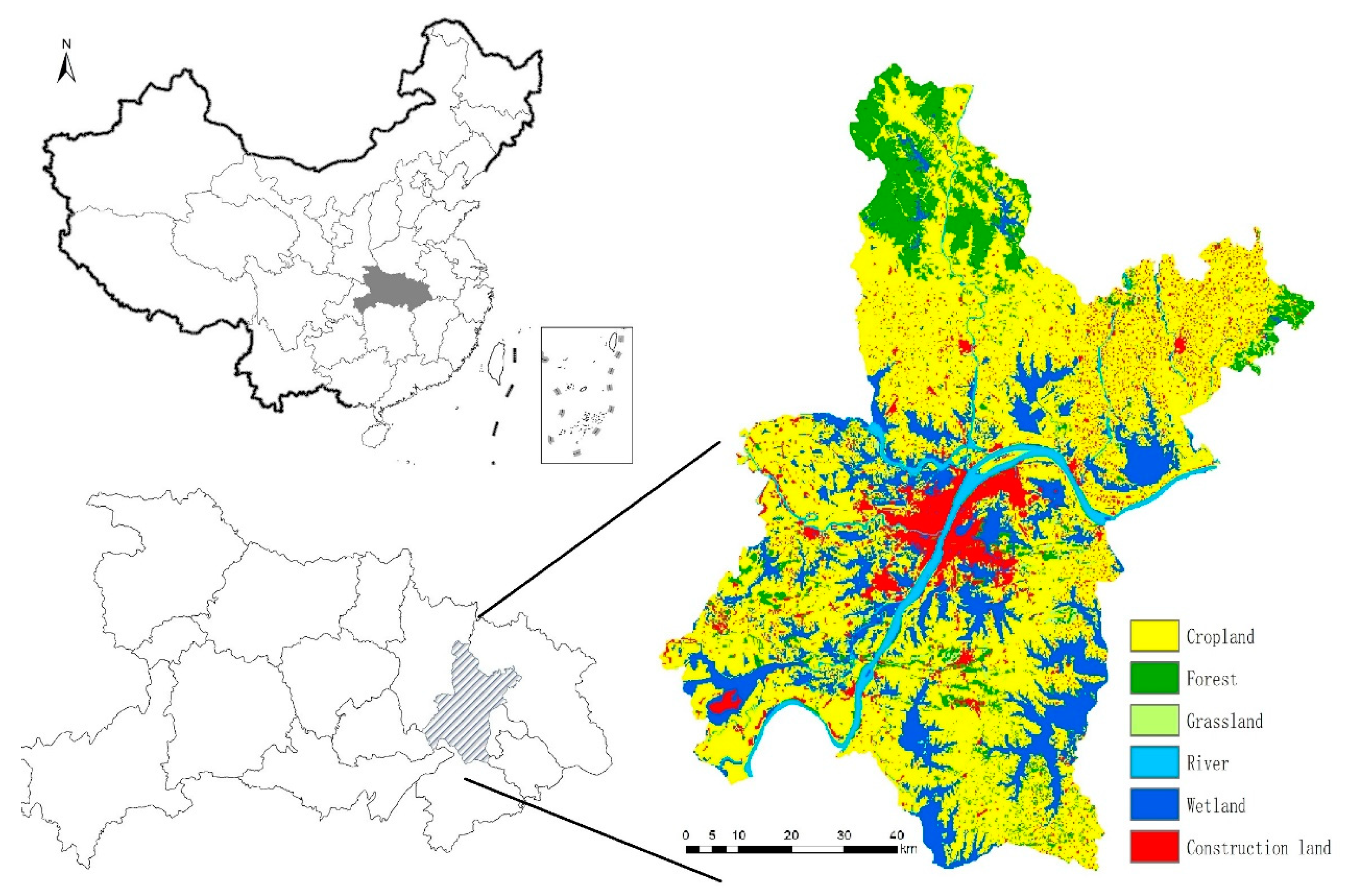
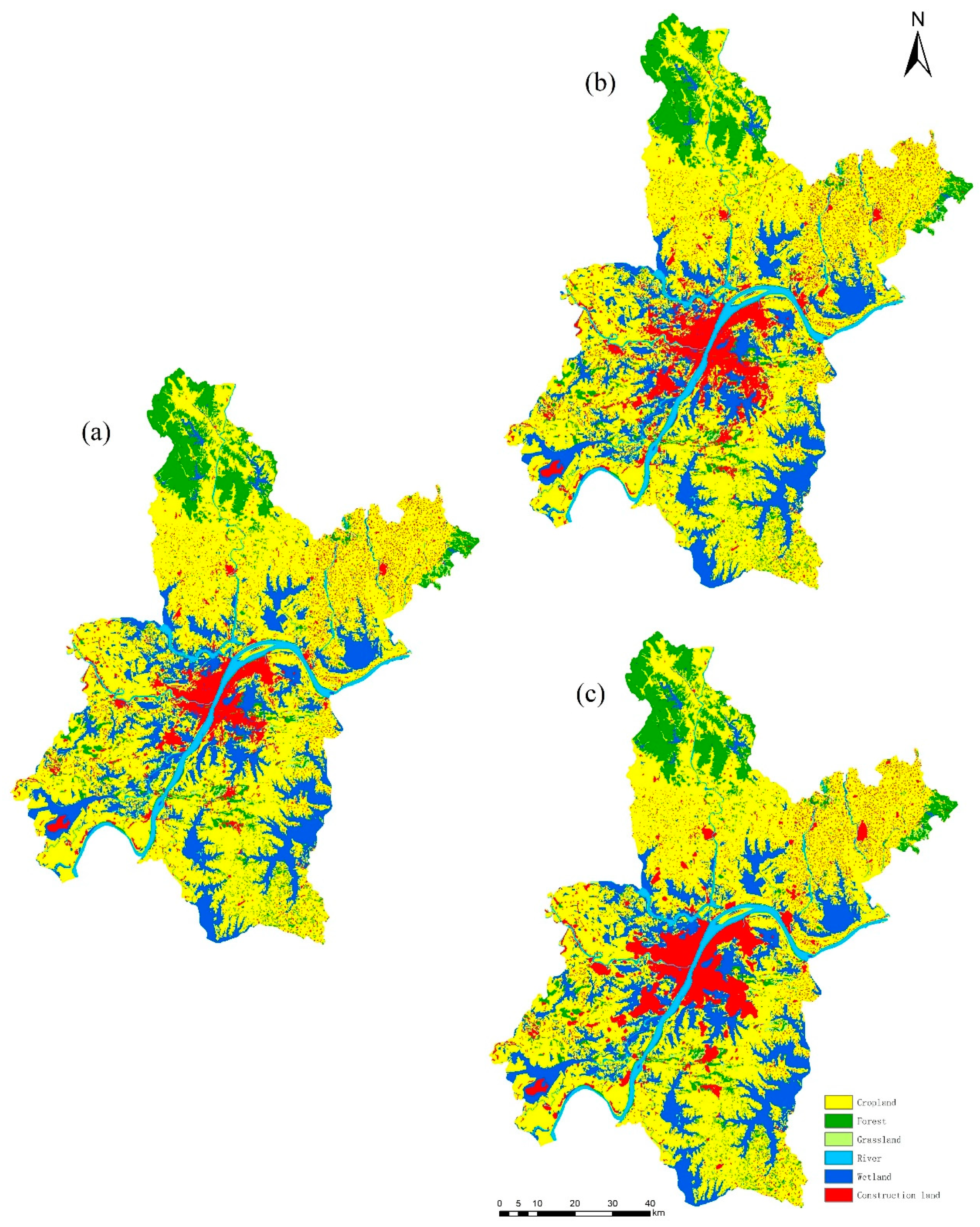
To address this gap in the literature, this study aims to assess the trade-offs between EB and ESV under various cropland protection policy scenarios. Our analysis focuses on the City of Wuhan, a rapidly urbanizing megacity in central China that has witnessed massive changes in both land uses, and local and regional policies of urbanization and urban development. We first employed a land-use change model to simulate the growth in construction land and the displacement of cropland as well as other land use changes under three scenarios for cropland protection policies: (i) business as usual scenario (BAU) where there is no restriction of urbanization and no requirement for cropland protection; (ii) land use planning scenario (LUP) that involves a requirement for certain quantities of cropland in response to the land use planning policy of Wuhan 2006–2020; and (iii) cropland protection scenario (CLP) where cropland protection policies are implemented based on the increased cost of cropland conversion. Following this, we analyzed the trade-offs between the EB and ESV of land use based on these policy scenarios.

2. Method and Materials

2.1. Study Area

Wuhan is the leading city in Hubei province, China (Figure 1). According to the statistical yearbook of Wuhan in 2015, the population of Wuhan was estimated at 10.6 million, of which over 80% live in urban areas. Wuhan is the most important economic center in Hubei province as well as in central China. It also covers an area of more than 8494 km², which accounts for 5029 km² of intensive croplands. More than 160 lakes, 4 wetland parks, 16 mountains, 6 forest parks, etc. in Wuhan make the city an ecologically important one. As a city with an outstanding advantage in geographic location, Wuhan is a pilot city in China for resource-saving and environmental protection. Naturally, competition for land between ecological conservation, agricultural production, and urban expansion has become increasingly severe in Wuhan, which makes the city an ideal area for this study.

2.2. Method

2.2.1. The Land Use Change Model

Cellular automata (CA) consists of a series of cells that assume a certain status at any time. The time changes in discrete steps and all cells can change their status or their neighbor’s status according to a certain function of their transition rules and neighborhood effects [31]. Furthermore, CA models have been widely employed to project future land use trajectories because of their capacity of generating patterns and representing the nonlinear spatial random land use change progresses [32,33]. However, most of the CA-based models can only reveal the changes of one certain land use type (mostly urban). Thus, they fail to show the interactions and feedbacks among different land use types. The Land System Cellular Automata for Potential Effects (LANDSCAPE) model is a promoted CA-based model that has the ability to simulate multiple land use changes by introducing the hierarchical allocation strategy [34]. In addition, recently, several researchers have utilized the LANDSCAPE model to project future land use change [24,35].

The allocation of land use in the LANDSCAPE model is based on two key parameters: the hierarchical allocation strategy and transition probability [34]. According to the theory of hierarchical allocation strategy, different land use types are classified into two groups: active and passive groups [36]. In the active group, the driving factors of land use changes are socioeconomic demands, whereas land use types in the passive group are driven by the changes in the active ones. For example, the expansion of the construction land is to meet the human demand for developing, whereas the changes of wetland are driven by the changes of construction land. The transition probability is made up of two parameters, namely, suitability and resistance. Suitability refers to the quality of a pixel to be transformed into its objective. Resistance refers to the cost of a pixel to change its current situation. Based on suitability and resistance, the transition probability is based on the following equation:

$${\mathrm{TP}}_{\mathrm{m},\mathrm{n}}=\frac{{\mathrm{S}}_{\mathrm{m},\mathrm{n}}}{{\mathrm{R}}_{\mathrm{m},\mathrm{j}}}$$

(1)

where ${\mathrm{TP}}_{\mathrm{m},\mathrm{n}}$ is the probability for pixel $\mathrm{m}$ to be converted to its objective $\mathrm{n}$; ${\mathrm{S}}_{\mathrm{m},\mathrm{n}}$ is the suitability of pixel $\mathrm{m}$ for its objective $\mathrm{n}$; ${\mathrm{R}}_{\mathrm{m},\mathrm{j}}$ is the resistance of the pixel $\mathrm{m}$ to be transformed from its land use type $\mathrm{j}$.

In this study, the resistance of each land use type, shown in

Table 1. Resistance of each land use type.

Land Use Type	Cropland	Forest	Grassland	River	Wetland	Construction Land
Resistance	1	1.25	1.25	1.5	1.25	1.5

, is based on Ke et al. [37]. The suitability ${\mathrm{S}}_{\mathrm{m},\mathrm{n}}$ is calculated based on the following equation:

$${\mathrm{S}}_{\mathrm{m},\mathrm{n}}=\left(1+{\left(-\ln \mathsf{\beta }\right)}^{\mathsf{\delta }}\right)\times {\mathrm{EF}}_{\mathrm{m},\mathrm{n}}\times {\mathrm{Con}}_{\mathrm{m},\mathrm{n}}\times {\mathsf{\Omega }}_{\mathrm{m},\mathrm{n}}$$

(2)

where $\left(1+{\left(-\ln \mathsf{\beta }\right)}^{\mathsf{\delta }}\right)$ is a stochastic influence factor, representing the relationship between suitability and the parameters that cannot be explained by the variables; $\mathsf{\beta }$ is a stochastic number and δ is a dispersion factor to restrain $\mathsf{\beta }$; ${\mathrm{EF}}_{\mathrm{m},\mathrm{n}}$ is the impacts of environmental factors on suitability, including slope, distances to roads, soil matters, etc. ${\mathrm{Con}}_{\mathrm{m},\mathrm{n}}$ is the constraint of pixel $\mathrm{m}$ to be transformed into objective $\mathrm{n}$. ${\mathsf{\Omega }}_{\mathrm{m},\mathrm{n}}$ is neighborhood effect.

2.2.2. Model Calibration

According to Ke et al. [34], the calibration progress of the LANDSCAPE model can be summarized in the following steps: (i) decide the active and passive land uses and figure out the demand of each active land use; (ii) reveal transition probability for each active land use; (iii) project land use change in the calibration stage. In this study, we calibrated the LANDSCAPE model by simulating the land use map in 2013 based on the land use map in 2000.

Kappa simulation was used to test the reliability of the LANDSCAPE model. Unlike the traditional Kappa index, the Kappa Simulation has the advantage of distinguishing the changed and unchanged pixels according to the land use map both at the original and the end of the simulated period and only assessing the accuracy of the changed pixels [38]. The value of the Kappa simulation score ranges from −1 to 1, and a land use type with a score bigger than 0 means the probability of reliability of the simulation results; whereas a score closer to 1 means a higher confidential level.

2.2.3. Scenario Development

To explore the impacts of different cropland protection policies on the trade-offs between EB and ESV, three policy scenarios have been developed. In each scenario, we simulated a series of land use changes caused by the growth in construction land with an interval of 5000 ha. In the first simulation, the initial land use map is the land use map of 2013, and the demand for construction land is the demand in 2013 plus 5000 ha. In the second simulation, the basic data is the simulation results of the first simulation, and the demand for construction land is the demand in the first simulation plus 5000 ha. As for the next simulations, the basic data and the demand for construction land are obtained by the same methods.

The first land use policy scenario, denoted business as usual scenario (BAU), assumes that there are no policies to restrain the development of construction land. The second scenario, termed land use planning scenario (LUP), assumes that the quantity of cropland follows the constraint of land use planning of Wuhan 2006–2020. The third scenario, denoted cropland protection scenario (CLP), aims to reduce the loss cropland during urbanization. The cropland protection scenario is based on the cropland protection policies which have been implemented since 1997. Further, the land use planning scenario is developed according to the land use planning of Wuhan in 2006–2020, which restrains the minimum area of cropland. We didn’t consider the effects of stakeholders in the scenario development. Different combinations of demands and resistances were used to identify these scenarios (

Table 2. The demands and resistances of land uses in different scenarios.

		Cropland	Forest	Grassland	River	Wetland	Construction Land
Initial	Amount	470,616	78,273	13,847	30,396	153,089	104,385
BAU	Demand	-	-	-	-	-	Dynamic
	Resistance	1	1.25	1.25	1.5	1.25	1.5
LUP	Demand	338,000	-	-	-	-	Dynamic
	Resistance	1	1.25	1.25	1.5	1.25	1.5
CLP	Demand	-	-	-	-	-	Dynamic
	Resistance	1.5	1.25	1.25	1.5	1.25	1.5

BAU: business as usual scenario; LUP: land use planning scenario; CLP: cropland protection scenario.

).

In the BAU scenario, there were no demands for land use types except construction land. Moreover, the resistances used during each simulation were the same as the calibration period since there were no constraints for the expansion of construction land. To identify the demand for cropland in the LUP scenario, we relied on the land use planning of Wuhan 2006–2020, which states that an amount of cropland of 338,000 ha will be needed. The resistances in the LUP scenario were set as the same as that in the calibration progress. In the CLP scenario, the demands for cropland, forest, grassland, river and wetland were not given too. Thus, to reduce the loss of cropland, the resistance of cropland was set as that of construction land, representing the increased cost of cropland conversion.

2.2.4. Economic Benefits Calculation

Each land use type has its economic output. The economic benefits refer to the return of assets or economic activities [39]. Therefore, we used the gross domestic product of the primary industry (GDPPI) to represent the EB of cropland, forest, grassland, wetland, and river. Two major EBs were calculated in this study: from construction land and the primary industry.

To calculate the EB of construction land, we used the Cobb–Douglas (C–D) production function to measure the economic efficiency of land while controlling the multicollinearity among the explanatory variables [40]. This production function is extensively applied to measure the relationship between the input and output factors. The form of this function we used in this research is shown in Equation (5):

$${\mathrm{EB}}_{\mathrm{j}}={\displaystyle \prod }{\mathrm{FC}}_{\mathrm{i}}^{{\mathrm{a}}_{\mathrm{i}}}\times {\mathrm{LD}}_{\mathrm{j}}^{{\mathrm{b}}_{\mathrm{j}}}$$

(3)

where ${\mathrm{EB}}_{\mathrm{j}}$ (j refers to construction land in this research) is the economic benefits of a specific land use; FC_i is the i-th input factors (i refers to labor and capital investment in this research); ${\mathrm{a}}_{\mathrm{i}}$ is the associated coefficient of ${\mathrm{FC}}_{\mathrm{i}}$; ${\mathrm{LD}}_{\mathrm{j}}$ is the area of a specific land use type; and ${\mathrm{b}}_{\mathrm{j}}$ is the associated coefficient of ${\mathrm{LD}}_{\mathrm{j}}$.

The log-transformed functional form is:

$$\ln {\mathrm{EB}}_{\mathrm{j}}={\displaystyle \sum }\left({\mathrm{a}}_{\mathrm{i}}\times \ln {\mathrm{FC}}_{\mathrm{i}}\right)+{\mathrm{b}}_{\mathrm{j}}\times \ln {\mathrm{LD}}_{\mathrm{j}}$$

(4)

With the log-transformed form, the coefficients can be estimated. The estimation results of the parameters are shown in

Table 3. Estimated Cobb–Douglas (C–D) production function for construction land and cropland.

Variable	Measurement Unit	Coefficient Estimate	Standard Error
Labor	Ten thousand persons	0.772 **	0.300
Capital investment	One hundred million yuan	0.469 ***	0.081
Quantity of construction land	ha	1.184 **	0.435
Adjusted R-Squared		0.998

*** Significant at 1%. ** Significant at 5%.

.

We used the land use efficiency to estimate the EB of cropland, forest, grassland, river and wetland, as shown in Equation (5).

$${\mathrm{EB}}_{\mathrm{n}}={\mathrm{LUE}}_{\mathrm{ave}}\times {\mathrm{LD}}_{\mathrm{n}}$$

(5)

where ${\mathrm{EB}}_{\mathrm{n}}$ is the EB of cropland, forest, grassland, river, and wetland, which also means the GDPPI; ${\mathrm{LUE}}_{\mathrm{ave}}$ is the average land use efficiency of cropland, forest, grassland, river, and wetland from 2000 to 2015; ${\mathrm{LD}}_{\mathrm{n}}$ is the total area of cropland, forest, grassland, river, and wetland.

The calculation of ${\mathrm{LUE}}_{\mathrm{ave}}$ was shown in the follows:

$${\mathrm{LUE}}_{\mathrm{ave}}={\displaystyle \sum }\frac{{\mathrm{GDPPI}}_{\mathrm{i}}}{{\mathrm{LD}}_{\mathrm{i}}}/\mathrm{N}$$

(6)

where ${\mathrm{GDPPI}}_{\mathrm{i}}$ is the i-th year of GDPPI; ${\mathrm{LD}}_{\mathrm{i}}$ is the quantity of cropland, forest, grassland, wetland, and river in the i-th year; N is the number of years, which is 16 because we chose the GDPPI data from 2000 to 2015.

2.2.5. Evaluation of Ecosystem Services Value

Ecosystems have been recognized as the basic condition for social development and human survival [41]. However, only until the 1970s, it has been recognized objectively and before that, it was considered as abundant and no-cost resources [42]. The growing awareness about ecosystem functions and ecological protection makes the evaluation of the ESV of land use a formal and continual theme since the 1990s [10,12,43]. Costanza et al. [12] evaluated the value of 17 global ecosystem services using money transfer method based on global LULC data and unit value; however, this evaluation results were found to be inappropriate for the Chinese context. Thus, Xie et al. [44] upgraded Costanza’s work and proposed a dynamic method for assessing the ESV of China. They evaluated the value of China’s ecosystem services for 2010 as a base year according to the MA framework and estimated the equivalent coefficients of six ecosystems (cropland, forest, grassland, wetland, barren land, and water area) and four ecosystem services (provisioning services, regulating services, habitat services, cultural and amenity services) [44]. The economic benefits of each ecosystem were provided by the provisioning services. Therefore, we didn’t consider the provisioning services to avoid double-counting when calculating the total ESV. The equivalent coefficients were based on the survey from 500 Chinese ecological experts, during which the standard equivalent factors were decided by three methods: (i) direct comparison with the previous studies; (ii) indirect comparison with ecosystem biomass; and (iii) experts’ knowledge [44].

In this study, the total ESV of land use was estimated as follows:

$$\mathrm{ESV}={\displaystyle \sum }\left({\displaystyle \sum }{\mathrm{EC}}_{\mathrm{ij}}\times \mathrm{SEF}\times {\mathrm{LD}}_{\mathrm{i}}\right)$$

(7)

where ESV is the sum ecosystem services value of the research area; ${\mathrm{EC}}_{\mathrm{ij}}$ is the equivalent coefficient of per unit area of the j-th ecosystem service for the i-th land use type; $\mathrm{SEF}$ is the standard equivalent factor; and ${\mathrm{LD}}_{\mathrm{i}}$ represents the quantity of the i-th land use type. The standard equivalent factor applied in this study is 503.2 USD/ha and the equivalent coefficient is shown in

Table 4. The equivalent coefficient for ecosystem services value (ESV) per unit area of ecosystem services for each land use and ecosystem service.

	Cropland	Forest	Grassland	Wetland	River
Regulating services	4.77	18.19	15.3	35.82	111.85
Habitat services	0.21	2.41	2.18	7.87	2.55
Cultural and amenity services	0.19	1.06	0.96	4.73	1.89

.

2.3. Data Sources

Data from five main datasets were used in this study. Four of them are spatial datasets: land use datasets, accessibility datasets, meteorological datasets, and soil datasets, and the fifth is a statistical economic dataset: the economic datasets. The spatial datasets are used by the LANDSCAPE model to calculate the parameters needed in the simulation and to calibrate the model. Land use datasets, including two phases of land use data: 2000 and 2013, and 6 land use types: cropland, forest, grassland, river, wetland, and construction land, were obtained from the land use database of the Data Center of Resources and Environment, Chinese Academy of Science (http://www.resdc.cn/). The accessibility datasets were firstly vectorized from the Traffic Atlas of Wuhan and then we used the Euclidean Distance Tool to generate the distance raster of each cell’s accessibility. The meteorological datasets were downloaded from the National Meteorological Information Center (http://data.cma.cn/), including average annual cumulative temperature data and annual precipitation data. The soil datasets consisted of soil phosphorus content, soil PH and soil organic matter content and there were compiled from China Soil Database (http://gis.soil.csdb.cn/). To unify the spatial resolution, all the spatial datasets were resampled to a resolution of 100 m.

The economic datasets included two sub-datasets: construction land datasets and primary industry datasets. The former consisted of the labors in the second and tertiary industries, capital investment in the urban area and the quantity of construction land. The latter was made up of the gross domestic product (GDP) of the primary industry. All datasets were obtained from Wuhan Statistical Yearbook from 2000 to 2015 (http://tjj.hubei.gov.cn/).

3. Results

3.1. Results of the LANDSCAPE Model Calibration

Figure 2 portrays the land use map of the study area for the observed year 2000, and the simulated results for 2013. The simulated result is relatively centralized. Compared to the real land use map of 2013, the construction land is particularly clustered in the central area. A look at the results of Kappa Simulation in

Table 5. Kappa simulation score for the calibration results.

	Cropland	Forest	Grassland	Wetland	Construction Land
Kappa Simulation	0.215	0.181	0.152	0.126	0.312

indicates that the score of each land use type is greater than zero, implying a high accuracy of the simulation result. Notably, the result points out that the active land use types have higher Kappa simulation scores while the passive land use types have relatively lower scores.

3.2. The Land Use Change Results in the Scenarios

Figure 3 displays the areas of cropland, forest, grassland, and wetland that were occupied by construction land in each simulation under different scenarios. The results point out to distinguishable land use transform patterns across scenarios. In the BAU scenario (Figure 3a), cropland is the main land use type occupied by the construction land and it conforms to a decreasing sequence from the first simulation to the last. In the first three simulations, construction land expansion only takes up cropland. From the fourth simulation onward, construction land begins to occupy other lands in the sequence of grassland, forest, and wetland. Specifically, wetland conforms to an increasing contribution to the construction land expansion. After the thirty-sixth simulations, the area losses of cropland and wetland are almost equal in each simulation.

With respect to LUP scenario, the results indicate that until the 27^th simulation, the land use change pattern of this scenario is almost consistent with that in the BAU scenario. After that, land use change pattern begins to vary (Figure 3b). In the first 27 simulations, the total loss of cropland is 132,616 ha and the area of the remaining cropland is 338,000 ha, which corresponds to the cropland demand in the LUP scenario. Accordingly, there is no loss in cropland area in the next 20 simulations. Forest and wetland are the two main land use types that were occupied by construction land in these simulations. However, a loss in cropland began again after the 47^th simulation.

Concerning the CLP scenario, the results shown in Figure 3c provide a quite different picture from those in the previous two scenarios. Specifically, there is no loss in cropland in the first 15 simulations, and the expansion of construction land takes in forest, grassland, and wetland. Moreover, forest conforms to a decreasing sequence, while wetland conforms to an increasing sequence. Starting from the 16^th simulation, cropland steadily begins to decrease to become, as from the 17^th simulation, the most important contributor to the construction land expansion. There are few simulations without wetland loss during the 19^th simulation and 30^th simulation. After that, a loss in wetland restarts, and the contribution rate of cropland to construction land expansion begins to decrease.

According to

Table 6. Loss in land use types in each scenario during the whole simulation progresses.

		Cropland	Forest	Grassland	Wetland
BAU	Quantity (ha)	184,458	11,259	8175	46,108
	Proportion (%)	73.8	4.5	3.3	18.4
LUP	Quantity (ha)	132,041	35,584	12,022	70,353
	Proportion (%)	52.8	14.2	4.8	28.1
CLP	Quantity (ha)	129,000	32,931	9830	78,239
	Proportion (%)	51.6	13.2	3.9	31.3

BAU: business as usual scenario; LUP: land use planning scenario; CLP: cropland protection scenario.

, the total losses of cropland, forest, grassland, and wetland during the whole progress are estimated for the BAU scenario at 184,458 ha (73.8%), 11,259 ha (4.5%), 8,175 ha (3.3%) and 46,108 ha (18.4%), respectively. The corresponding total loses for the LUP scenario were 13,2041 ha (52.8%), 35,584 ha (14.2%), 12,022 ha (4.8%), and 70,353 ha (28.1%). Concerning the CLP scenario, these numbers were estimated at 129,000 ha (51.6%), 32,931 ha (13.2%), 9,830 ha (3.9%), and 78,239 ha (31.3%), respectively.

3.3. Impacts of Different Policies on Trade-Offs between EB and ESV of Land Use

The curve (L₁) in Figure 4 demonstrates the trade-off between EB and ESV of land use in the BAU scenario. It indicates that an increase in EB of land use would lead to a decrease in ESV. Furthermore, it is obvious that the relationship between EB and ESV varies across different scales of urban expansion. Based on the scale of urban expansion and the slope of the curve, we divide the curve into two stages: stage 1 includes points before T¹; stage 2 represents the points after T¹. The slope of the curve is almost flat in stage 1. However, it goes sharply down in stage 2. This implies that the ecological cost for EB of land use is relatively lower in stage 1 and that it increases dramatically when the urban expansion goes beyond stage 1.

In relation to the land use change pattern in the BAU scenario (

Table 7. The average change of the occupied land in different stages in each simulation of the scenarios.

		BAU	LUP	CLP
Stage 1	Cropland	4630	4727	335
	Forest	129	76	1520
	Grassland	196	192	381
	Wetland	46	6	2764
Stage 2	Cropland	2155	192	4584
	Forest	383	1458	191
	Grassland	111	298	151
	Wetland	2352	3051	75
Stage 3	Cropland	-	-	2587
	Forest	-	-	248
	Grassland	-	-	35
	Wetland	-	-	2131

BAU: business as usual scenario; LUP: land use planning scenario; CLP: cropland protection scenario.

), construction land occupies cropland, forest, grassland, and wetland in stage 1 with averages of 4630 ha, 129 ha, 196 ha, and 46 ha, respectively. Moreover, Table 7 shows that during stage 1 cropland contributes the most to construction land. In stage 2, wetland suddenly takes over and becomes the biggest contributor (2352 ha in each simulation) in terms of contribution to construction land grasps. Moreover, it eventually reduces the cropland average amount of occupation to 2155 ha. Furthermore, the results point out that as long as cropland is the major land type swallowed by urban expansion, the ESV of land use decreases slowly. However, when urban expansion comes at the expense of ecological cost, the ESV of land use falls sharply. Thus, T¹ is the turning point in the BAU scenario.

Regarding the LUP scenario, the L₂ in Figure 4 shows that the conflict between EB and ESV of land use is severer than that in the BAU scenario. Like in the previous scenario, we divided this curve into two stages. In stage 1, just like the curve in the BAU scenario, the slope of the curve is almost flat. This implies that during stage 1, an increase in EB comes at a small cost of ESV. However, after T², the curve goes down sharply, and its inclination increases greatly and immediately. At stage 1, cropland devotes 4727 ha to construction land, almost 94.5% of the total devoted land (Table 7). Occupation of forest, grassland, and wetland appears to be slight. However, the contribution of cropland largely shrinks in Stage 2 to 192 ha, and by contrast, wetland contributes the most of the urban expansion swiftly from 6 ha at stage 1 to 3051 ha at stage 2 (Table 7). It is obvious that the increases of EB are at very low cost to ESV of land use in the early urbanization under the LUP scenario, but when EB reaches a certain stage, ESV of land use deteriorates by a large amount unexpectedly. So, a small increase in EB costs a great decrease in ESV. T² is just an obvious boundary between the two extremes.

Concerning the CLP scenario, the results presented by the curve (L₃) in Figure 4 suggest that the conflict between EB and ESV in this scenario is the severest among the three scenarios. Here, the curve (L₃) can be split into three stages according to the scale of urban expansion and its slope: stage 1 represents the points before T³; stage 2 marks the points between T³ and T⁴; stage 3 represents the points after T⁴. The slope of the curve in stage 1 in the CLP scenario is steep and it thus differs from that in the BAU and LUP scenarios. In stage 3, the curve however becomes steep again. That is, the ecological cost for EB is very high in the CLP scenario even at a small scale of urban expansion, and after a certain amount of urban expansion, the ecological cost of EB decreases sharply. With the continuation of urban expansion, the ecological cost rises sharply again. The land use change pattern in the CLP scenario is utterly different from that in the BAU and LUP scenarios (Table 7). In the BAU and LUP scenarios, cropland is the major land use type occupied by construction land, while in the CLP scenario, wetland and forest contribute 2764 ha and 1520 ha to construction land in stage 1 with a sharp reduction of 335 ha of cropland. In stage 2, cropland regains its position to become the main land use type taking up about 4584 ha, which then makes the slope of the curve flatter. With an average 2131 ha, wetland utilized for construction land finally breaks the flat and slants the curve more steeply again in stage 3. Thus, it could be concluded that, under the CLP scenario, a one-step increase in EB would worsen the ESV of land use greatly at the beginning of urbanization. However, when urban expansion develops to a certain stage (T³ is exactly the key turning point), the impact of urbanization on ESV of land use turns out to be negligible. In this context, EB and ESV of land use could coexist harmoniously. But further progress in EB would ruin the relationship between EB and ESV of land use (T⁴ is another turning point).

4. Discussion

Since the 1990s, the strictest cropland protection policies have been put into practice by the Chinese government, which occupies a vital position in food security for both China and the whole world [20]. On the one hand, these policies have been successful in achieving their original goal of mitigating the pressure of the quantity loss of cropland [28,45]. On the other hand, these policies have failed in several aspects such as the compensation for the loss in crop productivity and the increasing ecological cost [46]. These conflicting impacts of cropland protection policies have stimulated a growing strand in the literature that assess trade-offs between economic and ecosystem services [47,48]. The study contributes to this literature stream by providing evidence from the rapidly urbanizing city of Wuhan in China on the trade-offs between EB and ESV under three policy scenarios. Our results confirm the findings of previous studies showing that trade-offs between economic and ecosystem services are not constant as they have temporal and spatial heterogeneity [49]. Furthermore, we demonstrate that the trade-off between economic and ecosystem services is dynamic in urbanization processes and these trade-offs widely vary under different cropland protection policies. This finding goes in line with Costanza et al. [43] and de Groot et al. [50] who pointed out that LULC changes are closely related to the change of ESV and EB and land use policies lead to changes in land uses. Moreover, our results pay support to Hauer et al. 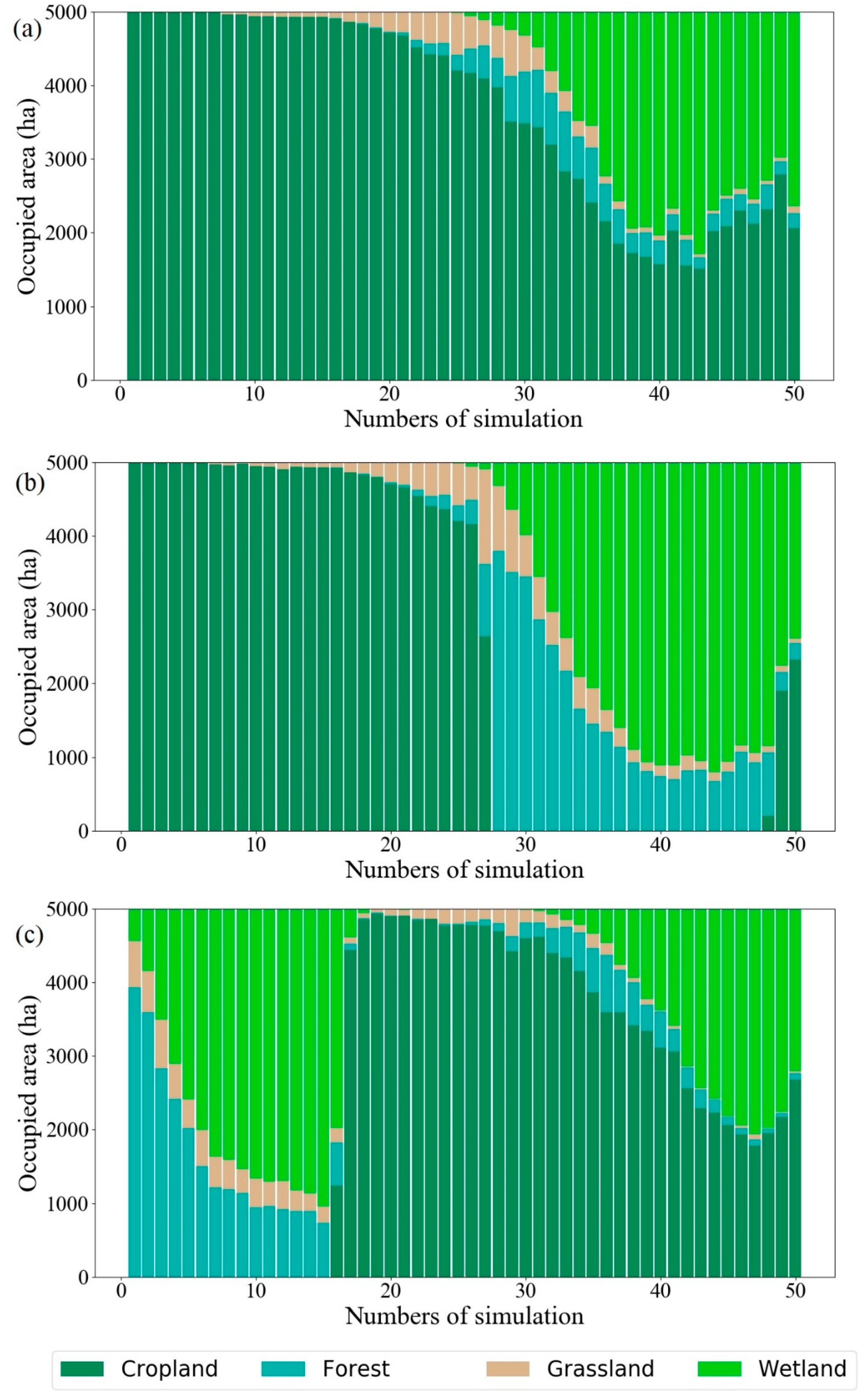[48] who showed that different land use policies differently affect the relationship between EB and ESV of land use. More specifically, the results of our three policy scenarios showed that trade-offs between EB and ESV in both the BAU and LUP scenarios, remain at moderate levels during the beginning of urban expansion processes. However, at certain ‘turning point’, the ESV decreases sharply whereas the EB slightly increases. Before this turning point, the increases in construction land are mainly due to the conversion of cropland, which has a relatively lower ESV because construction land is surrounded by cropland. After the turning point, land uses with high ESV are taken up by construction land. In the CLP scenario, the difficulty of cropland conversion increased due to the cropland protection policy. The transition probabilities of cropland to construction land become relatively lower, compared with the similar locations of wetland and forest. Thus, before the first turning point in the CLP scenario, forest and wetland with relatively higher ESV are the main land use types converted to construction land, leading to a mild increase of EB with a sharp decrease of ESV. When the transition probabilities of the remaining forest and wetland are lower than those of the remaining cropland, the construction land begins to consume cropland (points between T³ and T⁴, Figure 4). 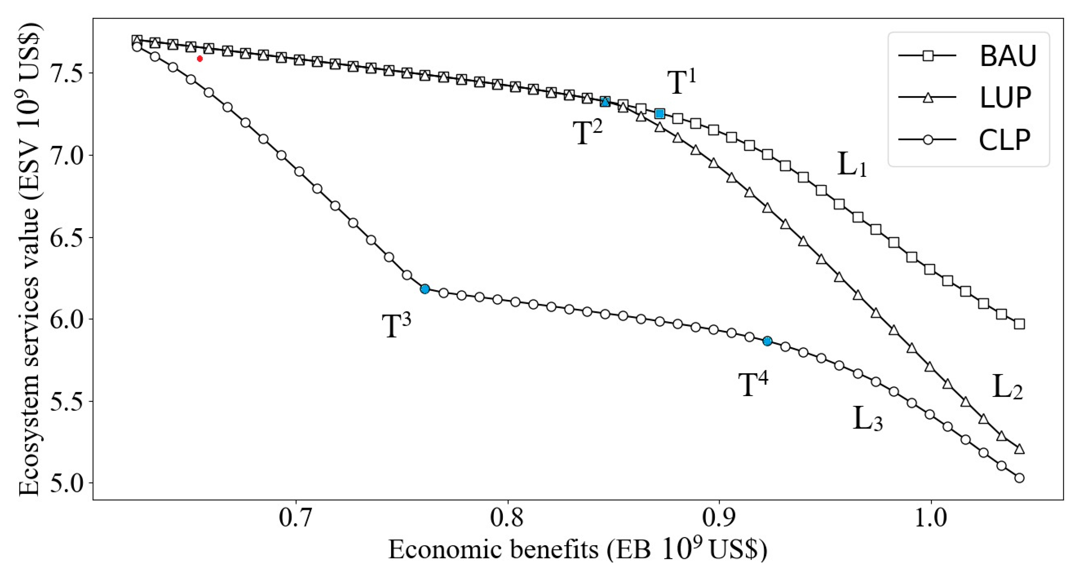These changes indicate also that when the rate of land use change is constant, the key factor driving the changes of ESV is the transfer direction [30,51]. Therefore, our results overall show that the numbers and positions of these turning points differ across the three policy scenarios (Figure 4).

Based on our findings, the ESV in the CLP scenario is the lowest among the three scenarios with the same level of EB. Moreover, the change in the relationship between EB and ESV (Figure 4) indicates that the cropland protection policy aggregates the trade-offs between EB and ESV of land use. Therefore, it is crucial for cities experiencing rapid urbanization processes to consider unleashing the restriction of taking up cropland and compensating cropland across cities or provinces. The red point is the situation of Wuhan in 2015, which is far away from all the turning points. However, policymakers should take this result into consideration when deciding on policies to be implemented in the future.

Spatial planning and land use planning perform important roles in a city and dealing with trade-offs among landscapes, natural resources and stakeholders. Reasonable spatial planning may avoid unnecessary loss of ecological land and relieve the trade-offs between the EB and ESV [52]. In our study, the trade-offs between EB and ESV in the LUP scenario are less drastic than those in the CLP scenario, which reveals that compared with the cropland protection policy, land use planning in Wuhan delivers fewer negative effects on the relationship between EB and ESV of land use. Since the improvement in the efficiency of construction land allocation and the utilization of land resources is necessary, the government cannot allow unlimited growth in construction land [40]. It is better for the stakeholders to seek the equilibrium between food security, ecological conservation and urban development through the allocation and intensive use of construction land by scientific spatial planning.

Lastly, this research has some limitations that need further discussion. Firstly, the future economic benefits and ecosystem services are affected by many factors and these factors will change over time. In this research, we only focus on the change of EB and ESV caused by land use changes, while keeping other factors constant. Thus, this research can only predict the future trend of EB and ESV affected by land use rather than their accurate changes. Secondly, China is currently implementing a strict cropland protection policy which necessitates no loss of cropland quantity. In the CLP scenario, we just increased the difficulty of cropland transition and allowed the occurrence of cropland loss. That is why we denoted this scenario ‘cropland protection scenario’ but strictly speaking it is not a strict cropland protection. Third, we evaluate the ESV of land use based on Xie et al. [44] and this method has a disadvantage as it omits the spatial heterogeneity of ecosystem services [10]. Although our study area covers a small range, the species and their ages within the same land use type do exist heterogeneity.

5. Conclusions

This paper assessed the trade-offs between EB and ESV in the Chinese city of Wuhan under three cropland protection policy scenarios. The LANDSCAPE model was employed together with the C-D production function and unit value-based methods. Our findings suggest that trade-offs between EB and ESV would change under the different levels of urbanization and it could also change with the impacts of different policies. It explains the trade-offs between economic and ecosystem services are not always severe; in some levels of urbanization, they would be trifling. These trade-offs became more pronounced in the CLP scenario, as there was more loss of forest and wetland due to the cropland protection policy. The results indicated that we should control the quantity of construction land to a certain extent and try to explore cropland compensation between cities or provinces, minimizing the loss of ecosystem services as much as possible.

References

1. Abu Hatab, A.; Cavinato, M.E.R.; Lindemer, A.; Lagerkvist, C.J. Urban sprawl, food security and agricultural systems in developing countries: A systematic review of the literature. Cities 2019. [Google Scholar] [CrossRef]
2. UN. World Urban Prospects: The 2018 Revision—Key Facts; United Nations: New York, NY, USA, 2018. [Google Scholar]
3. Badreldin, N.; Abu Hatab, A.; Lagerkvist, C.J. Spatiotemporal dynamics of urbanization and cropland in the Nile Delta of Egypt using machine learning and satellite big data: Implications for sustainable development. Environ. Monit. Assess. 2019, 191. [Google Scholar] [CrossRef] [PubMed]
4. UN. Transforming our world: The 2030 Agenda for Sustainable Development; UN General Assembly: New York, NY, USA, 2015. [Google Scholar]
5. Bai, X.; Chen, J.; Shi, P. Landscape urbanization and economic growth in China: Positive feedbacks and sustainability dilemmas. Environ. Sci. Technol. 2012, 46, 132–139. [Google Scholar] [CrossRef] [PubMed]
6. Turok, I.; McGranahan, G. Urbanization and economic growth: The arguments and evidence for Africa and Asia. Environ. Urban. 2013, 25, 465–482. [Google Scholar] [CrossRef]
7. Luederitz, C.; Brink, E.; Gralla, F.; Hermelingmeier, V.; Meyer, M.; Niven, L.; Panzer, L.; Partelow, S.; Rau, A.L.; Sasaki, R.; et al. A review of urban ecosystem services: Six key challenges for future research. Ecosyst. Serv. 2015. [CrossRef] [Green Version]
8. Li, S.; Ma, Y. Urbanization, economic development and environmental change. Sustainability 2014, 6, 5143–5161. [Google Scholar] [CrossRef] [Green Version]
9. Johnson, B. Cities, systems of innovation and economic development. Innov. Manag. Policy Pr. 2008. [Google Scholar] [CrossRef]
10. Costanza, R.; de Groot, R.; Sutton, P.; van der Ploeg, S.; Anderson, S.J.; Kubiszewski, I.; Farber, S.; Turner, R.K. Changes in the global value of ecosystem services. Glob. Environ. Chang. 2014, 26, 152–158. [Google Scholar] [CrossRef]
11. Bratley, K.; Ghoneim, E. Modeling Urban Encroachment on the Agricultural Land of the Eastern Nile Delta Using Remote Sensing and a GIS-Based Markov Chain Model. Land 2018, 7, 114. [Google Scholar] [CrossRef] [Green Version]
12. Costanza, R.; D’Arge, R.; De Groot, R.; Farber, S.; Grasso, M.; Hannon, B.; Limburg, K.; Naeem, S.; O’Neill, R.V.; Paruelo, J.; et al. The value of the world’s ecosystem services and natural capital. Nature 1997, 387, 253–260. [Google Scholar] [CrossRef]
13. Bai, X. The urban transition in china: Trends, consequences and policy implications. In The New Global Frontier: Urbanization, Poverty and Environment in the 21st Century; Rutledge: London, UK, 2012; pp. 335–354. ISBN 9781849773157. [Google Scholar]
14. Gollin, D.; Jedwab, R.; Vollrath, D. Urbanization with and without industrialization. J. Econ. Growth 2016. [Google Scholar] [CrossRef]
15. Xiao, Y.; Song, Y.; Wu, X. How far has China’s urbanization gone? Sustainability 2018, 10. [Google Scholar] [CrossRef] [Green Version]
16. Wade, T.G.; Wickham, J.D.; Zacarelli, N.; Riitters, K.H. A multi-scale method of mapping urban influence. Environ. Model. Softw. 2009, 24, 1252–1256. [Google Scholar] [CrossRef]
17. Su, S.; Li, D.; Hu, Y.; Xiao, R.; Zhang, Y. Spatially non-stationary response of ecosystem service value changes to urbanization in Shanghai, China. Ecol. Indic. 2014, 45, 332–339. [Google Scholar] [CrossRef]
18. Seto, K.C.; Guneralp, B.; Hutyra, L.R. Global forecasts of urban expansion to 2030 and direct impacts on biodiversity and carbon pools. Proc. Natl. Acad. Sci. USA 2012. [Google Scholar] [CrossRef] [Green Version]
19. Tao, Y.; Li, F.; Liu, X.; Zhao, D.; Sun, X.; Xu, L. Variation in ecosystem services across an urbanization gradient: A study of terrestrial carbon stocks from Changzhou, China. Ecol. Model. 2015, 318, 210–216. [Google Scholar] [CrossRef]
20. Lichtenberg, E.; Ding, C. Assessing farmland protection policy in China. Land Use Policy 2008, 25, 59–68. [Google Scholar] [CrossRef]
21. Deng, X.; Huang, J.; Rozelle, S.; Zhang, J.; Li, Z. Impact of urbanization on cultivated land changes in China. Land Use Policy 2015, 45, 1–7. [Google Scholar] [CrossRef]
22. Liu, X.; Zhao, C.; Song, W. Review of the evolution of cultivated land protection policies in the period following China’s reform and liberalization. Land Use Policy 2017, 67, 660–669. [Google Scholar] [CrossRef]
23. Song, W.; Deng, X.; Yuan, Y.; Wang, Z.; Li, Z. Impacts of land-use change on valued ecosystem service in rapidly urbanized North China Plain. Ecol. Model. 2015, 318, 245–253. [Google Scholar] [CrossRef]
24. Ke, X.; Wang, L.; Ma, Y.; Pu, K.; Zhou, T.; Xiao, B.; Wang, J. Impacts of Strict Cropland Protection on Water Yield: A Case Study of Wuhan, China. Sustainability 2019, 11, 184. [Google Scholar] [CrossRef] [Green Version]
25. Jiang, W.; Deng, Y.; Tang, Z.; Lei, X.; Chen, Z. Modelling the potential impacts of urban ecosystem changes on carbon storage under different scenarios by linking the CLUE-S and the InVEST models. Ecol. Model. 2017, 345, 30–40. [Google Scholar] [CrossRef]
26. van Vliet, J.; Eitelberg, D.A.; Verburg, P.H. A global analysis of land take in cropland areas and production displacement from urbanization. Glob. Environ. Chang. 2017, 43, 107–115. [Google Scholar] [CrossRef]
27. Song, W.; Liu, M. Farmland Conversion Decreases Regional and National Land Quality in China. L. Degrad. Dev. 2017. [Google Scholar] [CrossRef]
28. Song, W.; Pijanowski, B.C. The effects of China’s cultivated land balance program on potential land productivity at a national scale. Appl. Geogr. 2013, 46, 158–170. [Google Scholar] [CrossRef]
29. Haase, D.; Schwarz, N.; Strohbach, M.; Kroll, F.; Seppelt, R. Synergies, trade-offs, and losses of ecosystem services in urban regions: An integrated multiscale framework applied to the leipzig-halle region, Germany. Ecol. Soc. 2012, 17. [Google Scholar] [CrossRef]
30. Wang, Y.; Dai, E.; Yin, L.; Ma, L. Land use/land cover change and the effects on ecosystem services in the Hengduan Mountain region, China. Ecosyst. Serv. 2018, 34, 55–67. [Google Scholar] [CrossRef]
31. Engelen, G.; White, R.; Uljee, I.; Drazan, P. Using cellular automata for integrated modelling of socio-environmental systems. Environ. Monit. Assess. 1995, 34, 203–214. [Google Scholar] [CrossRef] [Green Version]
32. Liu, X.; Liang, X.; Li, X.; Xu, X.; Ou, J.; Chen, Y.; Li, S.; Wang, S.; Pei, F. A future land use simulation model (FLUS) for simulating multiple land use scenarios by coupling human and natural effects. Landsc. Urban. Plan. 2017, 168, 94–116. [Google Scholar] [CrossRef]
33. Verburg, P.H.; Soepboer, W.; Veldkamp, A.; Limpiada, R.; Espaldon, V.; Mastura, S.S.A. Modeling the spatial dynamics of regional land use: The CLUE-S model. Environ. Manag. 2002, 30, 391–405. [Google Scholar] [CrossRef]
34. Ke, X.; Zheng, W.; Zhou, T.; Liu, X. A CA-based land system change model: LANDSCAPE. Int. J. Geogr. Inf. Sci. 2017, 31, 1798–1817. [Google Scholar] [CrossRef]
35. Zheng, W.; Ke, X.; Xiao, B.; Zhou, T. Optimising land use allocation to balance ecosystem services and economic benefits—A case study in Wuhan, China. J. Environ. Manag. 2019, 248, 109306. [Google Scholar] [CrossRef] [PubMed]
36. White, R.; Engelen, G. Cellular automata as the basis of integrated dynamic regional modelling. Environ. Plan. B Plan. Des. 1997. [Google Scholar] [CrossRef]
37. Ke, X.; van Vliet, J.; Zhou, T.; Verburg, P.H.; Zheng, W.; Liu, X. Direct and indirect loss of natural habitat due to built-up area expansion: A model-based analysis for the city of Wuhan, China. Land Use Policy 2018, 74, 231–239. [Google Scholar] [CrossRef]
38. van Vliet, J.; Bregt, A.K.; Hagen-Zanker, A. Revisiting Kappa to account for change in the accuracy assessment of land-use change models. Ecol. Model. 2011, 222, 1367–1375. [Google Scholar] [CrossRef]
39. Halati, A.; He, Y. Intersection of economic and environmental goals of sustainable development initiatives. J. Clean. Prod. 2018, 189, 813–829. [Google Scholar] [CrossRef]
40. Liu, Y.; Zhang, Z.; Zhou, Y. Efficiency of construction land allocation in China: An econometric analysis of panel data. Land Use Policy 2018, 74, 261–272. [Google Scholar] [CrossRef]
41. Braat, L.C.; de Groot, R. The ecosystem services agenda:bridging the worlds of natural science and economics, conservation and development, and public and private policy. Ecosyst. Serv. 2012, 1, 4–15. [Google Scholar] [CrossRef] [Green Version]
42. Turner, K.G.; Anderson, S.; Gonzales-Chang, M.; Costanza, R.; Courville, S.; Dalgaard, T.; Dominati, E.; Kubiszewski, I.; Ogilvy, S.; Porfirio, L.; et al. A review of methods, data, and models to assess changes in the value of ecosystem services from land degradation and restoration. Ecol. Model. 2015, 319, 190–207. [Google Scholar] [CrossRef]
43. Costanza, R.; de Groot, R.; Braat, L.; Kubiszewski, I.; Fioramonti, L.; Sutton, P.; Farber, S.; Grasso, M. Twenty years of ecosystem services: How far have we come and how far do we still need to go? Ecosyst. Serv. 2017, 28, 1–16. [Google Scholar] [CrossRef]
44. Xie, G.; Zhang, C.; Zhen, L.; Zhang, L. Dynamic changes in the value of China’s ecosystem services. Ecosyst. Serv. 2017, 26, 146–154. [Google Scholar] [CrossRef]
45. Zhong, T.; Huang, X.; Zhang, X.; Scott, S.; Wang, K. The effects of basic arable land protection planning in Fuyang County, Zhejiang Province, China. Appl. Geogr. 2012, 35, 422–438. [Google Scholar] [CrossRef]
46. Zheng, W.; Ke, X.; Zhou, T.; Yang, B. Trade-offs between cropland quality and ecosystem services of marginal compensated cropland – A case study in Wuhan, China. Ecol. Indic. 2019, 105, 613–620. [Google Scholar] [CrossRef]
47. Yang, W.; Jin, Y.; Sun, T.; Yang, Z.; Cai, Y.; Yi, Y. Trade-offs among ecosystem services in coastal wetlands under the effects of reclamation activities. Ecol. Indic. 2018, 92, 354–366. [Google Scholar] [CrossRef]
48. Hauer, G.; Cumming, S.; Schmiegelow, F.; Adamowicz, W.; Weber, M.; Jagodzinski, R. Tradeoffs between forestry resource and conservation values under alternate policy regimes: A spatial analysis of the western Canadian boreal plains. Ecol. Model. 2010, 221, 2590–2603. [Google Scholar] [CrossRef]
49. Rodríguez, J.P.; Beard, T.D.; Bennett, E.M.; Cumming, G.S.; Cork, S.J.; Agard, J.; Dobson, A.P.; Peterson, G.D. Trade-offs across space, time, and ecosystem services. Ecol. Soc. 2006. [Google Scholar] [CrossRef] [Green Version]
50. de Groot, R.; Brander, L.; van der Ploeg, S.; Costanza, R.; Bernard, F.; Braat, L.; Christie, M.; Crossman, N.; Ghermandi, A.; Hein, L.; et al. Global estimates of the value of ecosystems and their services in monetary units. Ecosyst. Serv. 2012, 1, 50–61. [Google Scholar] [CrossRef]
51. Han, Z.; Song, W.; Deng, X. Responses of ecosystem service to land use change in Qinghai Province. Energies 2016, 9. [Google Scholar] [CrossRef] [Green Version]
52. Salet, W.; Driessen, P.P.J.; Van Rijswick, M.; Spit, T.; Van Buuren, A.; Teisman, G.; Rietveld, P. Towards adaptive spatial planning for climate change: Balancing between robustness and flexibility. J. Eur. Environ. Plan. Law 2013. [Google Scholar] [CrossRef] [Green Version]
Figure 1. Location and land use of the study area.
Land 09 00117 g001
Figure 2. The land use map of the study area in the observed 2000 (a), 2013 (b) and the simulated results (c).
Land 09 00117 g002
Figure 3. The quantity of ecological land loss in each simulation in the scenarios of: (a) business as usual (BAU); (b) land use planning (LUP); and (c) cropland protection (CLP).
Land 09 00117 g003
Figure 4. The relationship between economic benefits and ecosystem services value in the scenarios of business as usual (BAU, L1), land use planning (LUP, L2), and cropland protection (CLP, L3). T1 is the turning point in the BAU scenario. T2 is the turning point in the LUP scenario. T3 and T4 are the turning points in the CLP scenario. The red point is the relationship between the economic benefits and ecosystem services value in Wuhan, 2015.
Land 09 00117 g004