Spatio-Temporal Evolution of Land Use Transition and Its Eco-Environmental Effects: A Case Study of the Yellow River Basin, China

Abstract

Human activities and environmental deterioration have resulted in land use transition (LUT), which seriously affects the ecosystem service value (ESV) of its region. Therefore, relevant policy measures are urgently needed. Nevertheless, research on the relationships between LUTs and ESVs from the overall watershed scale is lacking. Thus, the geo-information Tupu method was applied to analyze the dynamic patterns of LUT based on land use data from 1990, 2000, 2010, and 2018 of the Yellow River Basin (YRB). Then, a newly revised ecosystem services calculation method was utilized to the responses of ESV to LUTs. The results indicated that the Tupu units of the LUT were mainly based on the mutual transformation of grassland and unused land, and cultivated land and forestland, which were widely distributed in the upper and middle reaches of the basin. The spatial distribution was concentrated, and the expansion’s trend was also obvious. Moreover, the conversion of cultivated land into construction land was mainly distributed in the lower reaches of the basin. During 1990–2018, the total ESV fluctuated and increased (+10.47 × 10⁸ USD) in the YRB. Thereinto, the ESV of grassland (45%) and forestland (30%) made the greatest contribution to the total ESV. As for different reaches, the ESV increased in the upstream, but decreased in the midstream and the downstream. In terms of contribution rate, the conversion of unused land into grassland (12.477%) and grassland into forestland (9.856%) were the main types to enhance the ESV in the YRB, while the conversion of forestland into grassland (−8.047%) and grassland to unused land (−7.358%) were the main types to reduce the ESV. Furthermore, the range of ecological appreciation zones was widely distributed and scattered, while the range of ecological impairment zones was gradually expanded. These findings could have theoretical support and policy implications for land use planning and environmental services in the YRB.

1. Introduction

A watershed is an area where the natural environment and human activities interact strongly [1,2], and is also the main area of human life and reproduction. Statistically, the population of the world’s major basins is as high as 2.24 billion, accounting for about one-third of the world’s population. Human activities have resulted in dramatic land use transitions (LUTs), which have seriously affected the ecosystem services value (ESV). Then it would bring severe ecological problems that threaten sustainable human development [3,4,5]. It could be seen that the balance of the watershed ecosystem was easily affected by LUT, which posed a serious threat to the regional ecological environment. Therefore, it is necessary to model and analyze the impact of watershed ecosystem services. As the second-longest river in China and the fifth-longest river in the world [6,7], the Yellow River occupies important strategic positions both in social-economic development and as an ecological barrier in China [8]. However, the ecological environment of the Yellow River Basin (YRB, for short) is extremely fragile [9,10], which has been the focus and difficulty of watershed management in China since ancient times [6,11,12]. Notably, China’s Central Government has incorporated ecological protection and high-quality development of the YRB into the major national strategy [8]. Thus far, the YRB has not been well protected, mainly since the land use was not reasonable and the ESV was also ignored.

Land use/cover change (LUCC) is a vital part of global environmental change and sustainable development, which has long been a question of great interest in a wide range of fields [13,14]. As one of the manifestations of LUCC, LUT has been introduced as a new way to research land use change in different stages of socio-economic development, which attracted extensive attention of the academic community [15,16,17,18]. Recently, an increasing number of empirical studies have explored LUT, and the research scales are mostly concentrated in the whole country [19,20], urban agglomeration [5,7], city [21,22], and county [23]. The research content included theories and hypotheses, the transition of overall land use pattern and structure, driving mechanisms, the environmental effects, and the relationship between LUT and related socio-economic activities [15,16,17,24,25,26]. Therefore, future research on LUT would focus more on the impact on social economy and ecological environment, to compensate for the existing research on the ecological function of land use. Additionally, LUT analyses in previous studies have usually been based on the transfer matrix to yield the quantitative changes of land use and obtained a spatial distribution through overlay analysis of the land use data in different periods [27]. The geo-informatic Tupu method could record composite spatio-temporal information of land use change using Tupu units. Moreover, the spatial pattern and time sequence characteristics could also be quantitatively expressed under the multiple spatio-temporal conditions [4,5], which has gradually become an effective method to LUT.

Ecosystem services refer to the benefits that human beings directly or indirectly obtain from the ecosystem, including supplying services, regulating services, cultural services, and support services [28,29,30]. The ecosystem services are related to human well-being, and are the basis for human survival and social-economic development [28]. LUT was considered to be one of the main driving forces to change ecosystem services at regional and global levels [31,32], which had a significant effect on the regional natural environment and ecosystem [33,34]. Statistically, the loss of ESV was estimated between 4.3 to 20.2 trillion USD/year from 1997 to 2011 at the global level due to LUT [29]. In China as well, ESVs have been decreased due to high resource consumption and the city’s rapid expansion under economic development [22]. For example, ESV decreased by 0.45% (1988–2000) and 0.10% (2000–2008) [35]. Ecosystem services have been widely evaluated in the world [30,36]. Both the ESV and its comprehensive framework and principle for integrated assessment and evaluation have been studied in recent decades [13,28,37,38]. At present, three main approaches have been widely applied to assess ecosystem services, including equivalent factors, productivity, and biomass [28,39]. Among them, the equivalent factor method is more intuitive and easier to use, with fewer data requirements, comprehensive evaluation, and high comparability, and especially suitable for regional and global scale assessment [39].

Watershed, a natural catchment area, is a relatively independent and complete ecological unit with water as the core element [1,8]. It has become a basic consensus of the international community to study the ecological environment change from the overall level of the basin [40,41]. To explore the characteristics of LUT and its eco-environmental effects can provide scientific reference for ecological protection [42]. In the YRB, land use changes are a pervasive and common phenomenon [43], especially the continuous expansion of urban and rural construction land, and the space of agricultural and ecological land is squeezed [44], making the internal relationship of the natural ecosystem uncoordinated [45,46]. From the overall scale of the YRB, studying the response of ESV to LUT can provide an entry point for land management opportunities in the future. Furthermore, studies conducted on LUT in the YRB focus on the dynamics of cover changes and their causes [6,11,43] with little attention to address the impacts of such changes on the ecosystem services aspect.

The objective of this paper is threefold. The first is to assess the dynamic patterns of LUT in the YRB using the geo-information Tupu method. We use the change ratio and space separating degree to determine the spatio-temporal characteristics of Tupu change. The second is to evaluate the changes in ESV caused by LUT using the equivalent factor method. Thus, the ESV Tupu method was applied to further examine the response of ESV to LUT. The third is to discuss how to incorporate ecosystem services into land use policy implications. This paper contributes to the literature in several ways: (1) As for the research scale, this paper selects the special type of region as the research area. It could provide scientific guidance for the cross-regional collaborative governance by analyzing the ecological environment of the YRB from a systematic and holistic perspective. (2) As for the geographical space, this paper records the spatio-temporal composite information of land use change applying the geo-information Tupu method, and then systematizes and dynamizes the process of LUT and reveals its internal laws.

2. Materials and Methods

2.1. Study Area

The study site was the Yellow River Basin (YRB), located on China’s north at 95°53′ E–119°05′ E and 32°10′ N–41°50′ N, as shown in Figure 1. It is the second largest river in China, with a total length of 5464 km and a total area of 7.95 × 10⁵ km², accounting for 8.28% of the total area of China [47]. From west to east, the YRB flows through nine provinces and regions, namely Qinghai, Sichuan, Gansu, Ningxia, Inner Mongolia, Shaanxi, Shanxi, Henan, and Shandong. The topography in the YRB is dominated by hills, mountains, and plains, and the terrain is high in the west and low in the east. The YRB is dominated by a temperate continental monsoon climate with four distinct seasons and rich natural resources. In 2018, the total population of the YRB (nine provinces and autonomous regions) was 4.2 × 10⁸, accounting for 30.3% of China, and the GDP was 2.39 × 10¹³ yuan, accounting for 26.5% of the total national GDP. Referring to previous research [11], it was divided into upstream (Qinghai, Inner Mongolia, Ningxia, Gansu, Sichuan), midstream (Shaanxi and Shanxi), and downstream (Shandong and Henan).

2.2. Data Sources and Processing

Taking the administrative division in 2019 as the standard, the data of each year were unified to the administrative unit. There are there main sources of data: (1) The boundaries of the YRB, and provincial and municipal administrative units were based on the 1:250,000 basic geographic data provided by the Data Center for Resources and Environmental Sciences, Chinese Academy of Sciences (RESDC) (http://www.resdc.cn), including 9 provincial units and 76 municipal administrative units. (2) The land use data of the YRB in 1990, 2000, 2010, and 2018 were collected from the Data Center for Resources and Environmental Sciences, Chinese Academy of Sciences (RESDC) (http://www.resdc.cn) [19,48,49]. The data processing method was as follows. Firstly, the production of the data set was mainly based on Landsat Multi-Spectral Scanner (MSS), Thematic Mapper (TM)/ Enhance Thematic Mapper (ETM), and Landsat 8 remote sensing images as the data sources. With the help of ArcGIS, the geographical elements were mathematically and physically interpreted by manual visual interpretation, and the land use data with a spatial resolution of 30 × 30 m were generated. The original data included 6 major categories and 25 secondary subcategories [19]. After strict quality control, the overall identified accuracies of the primary type of land use reached 94.3%, and the classification accuracies of the secondary type reached more than 91.2% [19,49], which met the requirement of user mapping accuracy on the 1: 100,000 scale. Secondly, the vector data of the boundary of the YRB were used to mask the 30 m raster land use data of the whole country, and the spatial database of land use in the study area was constructed. The reclassify tool was used to reclassify the land use types, and the value of the extracted land type was Set 1, and that of other land types were Set No-data. (3) The grain yield data were derived from the statistical yearbooks of each province in the YRB from 1991 to 2019, and the grain price data were derived from the “China Agricultural Produce Survey Yearbook” in 2019.

Referring to the national standard of land use classification (GB/T21010-2007) in China, the land use types were classified into six types: cultivated land, forestland, grassland, water area, construction land, and unused land. Then, the land use data were recoded in ArcGIS 10.6. The cultivated land, forestland, grassland, water area, construction land, and unused land were set as 1, 2, 3, 4, 5, and 6, respectively, with a unified classification standard, as shown in Figure 2.

2.3. Geo-Information Tupu Methods

Tupu is a means to express content or transmit information by analyzing comprehensive maps, images, or tables [50]. It could effectively reflect the characteristics of spatial structure and spatio-temporal change. Geo-information Tupu is a geographic space–time analysis methodology [51], which could express various geographical elements through abstract mathematical forms [52]. Moreover, it could combine “TU expressing the characteristics of spatial unit” and “PU presenting the starting point and process of events”, which makes up for the deficiency of traditional data mining methods in thinking and space [53]. According to the theory and method of geo-information Tupu, based on land use data of four periods in the YRB, the paper employs a “Raster Calculator” to conduct map algebraic operations and builds series Tupu models for LUT.

2.3.1. Build the Process Tupu of LUT and ESV

The map algebraic superposition for LUTs’ Tupu unit was performed in ArcGIS 10.6 to integrate the spatial information of Tupu code [54]. Specifically, the codes of adjacent two-phase grid elements were selected for an algebraic operation to obtain the LUT Tupu value, seen in Formula (1):

$$C=10\times A+B$$

(1)

where C represents the Tupu code of the LUT during the research stage, A represents the land use unit code value in the previous stage, and B represents the land use unit code value in the later stage. Thus, the LUT Tupu of the YRB in 1990–2000, 2000–2010, and 2010–2018 can be obtained. Referring to existing studies [4,55], the Tupu of changes in ESV was obtained by multiplying the Tupu of LUT from 1990 to 2018 by the ESV per unit area of spatial grid. According to the change of ESV, the region was defined as an ecological preservation zone, ecological appreciation zone, and ecological impairment zone.

2.3.2. Statistics of the Tupu Characteristic

Characteristics of the “TU” are mainly the spatial representation of the sequential changing process of the land use Tupu unit, and the quantitative features of the Tupu unit type during the two sampling periods are the characteristics of the “PU” of the LUT [4,5]. In this study, the characteristics of “TU” in LUT are quantitatively presented by the degree of spatial separation, and the visual observation of the Tupu process in different stages. The characteristics of “PU” are represented by the sorted Tupu unit table. The specific formula of change ratio and spatial separation index [23,54,56] are as follows:

$$A_{ij}=N_{ij}\times 100\%/{\displaystyle \sum _{i=1}^n{\displaystyle \sum _{j=1}^n{N}_{ij}}}(i\ne j)$$

(2)

$$S_{ij}=\frac{1}{2}\times \frac{\sqrt{F_{ij}/{\displaystyle \sum _{i=1}^n{\displaystyle \sum _{j=1}^n{N}_{ij}}}}}{N_{ij}/{\displaystyle \sum _{i=1}^n{\displaystyle \sum _{j=1}^n{N}_{ij}}}}$$

(3)

where $A_{ij}$ represents change ratio. It presents the ratio of the transformed land use Tupu unit area to the total area of all transformed land use Tupu units. $S_{ij}$ represents the spatial separating degree, and reflects the degree of dispersion of the Tupu unit. $F_{ij}$, $N_{ij}$ refers to the number of Tupu units and area of land use types converted from the land use type $i$ at the initial stage to the land use type $j$ at the last stage, and $n$ represents the number of land use types.

2.4. Calculation of ESV

2.4.1. Revision of Value Coefficient

Since Costanza et al. [28] scientifically expounded the principles and methods of estimating ESV published in Nature, relevant studies had gradually become a hot topic in academia and widely used around the world [40,57]. However, there are some defects in the direct application in China, such as the estimation of the farmland is too low but the wetland is too high [35,58]. Therefore, from combined expert knowledge of more than 700 ecologists, Xie et al. [38] revised the ecosystem services classification and ecosystem equivalent table in China. The 17 ecosystem services proposed by Costanza et al. [28] were classified into four categories and nine sub-categories [38]. The equivalent value (EV) per unit area of food production of cultivated land was set to 1, and the EV of other ecosystem services can be quantified by comparing with the standard value of 1. Although some problems were still unsolved, it did not influence this method from being widely used by many scholars [35,58]. Therefore, this study adopted this method to further modify the ecological service coefficient according to the actual situation of the YRB.

As the land use types cannot correspond to ecosystem types one by one, this study chooses the closest land use type for equivalent valuation. The water area in this study included a water body and wetland, so this paper used the average equivalent ESV coefficients of water bodies and wetlands [38] to calculate the ESV. In this study, the ESV of construction land was assigned as zero [4]. The net profit of land use type production is regarded as the production value that the land use type can provide, and the net profit of food production per unit area of cultivated land is regarded as the ESV of one standard equivalent factor [39]. Generally, the economic value provided by natural ecosystems without human input is about 1/7 of the economic value of food provided by existing farmland per unit area [38]. According to the statistical yearbook of the provinces, the average grain yield of the YRB from 1990 to 2018 was 3987.98 kg/ (ha·a), and the grain purchase price was 0.47 USD/kg in 2018. Thus, the economic value of farmland grain yield provided by a standard equivalent factor in the YRB was calculated as about 267.76 (=3987.98 × 0.47 ÷ 7) USD/(ha·a). The value coefficients of ecological services provided by the modified ecosystems are shown in

Table 1. The ecosystem service value (ESV) per land use type after correction in the YRB.

Primary-Types	Secondary-Types	Cultivated Land	Forestland	Grassland	Water Area	Unused Land
SuyS	Food production	267.76	88.36	115.14	119.15	5.36
	Raw material	104.43	797.92	96.39	78.99	10.71
RegS	Gas regulation	192.79	1156.72	401.64	390.93	16.07
	Climate regulation	259.73	1089.78	417.71	2089.87	34.81
	Hydrological regulation	206.18	1095.14	407.00	4312.27	18.74
	Waste treatment	372.19	460.55	353.44	3915.99	69.62
SutS	Soil formation and retention	393.61	1076.40	599.78	321.31	45.52
	Biodiversity protection	273.12	1207.60	500.71	953.23	107.10
CulS	Recreation and culture	45.52	556.94	232.95	1222.32	64.26
Total		2115.30	7529.41	3124.76	13,404.07	372.19

. The equations are as follows:

$$ESV={\displaystyle \sum _{i=1}^{n}ES{V}_i}={\displaystyle \sum _{i=1}^n{P}_i\times A_i}$$

(4)

where ESV indicates the total ESV in the research area, i is the number of land use types (i = 1–6). ESV_i indicates the ESV of the ith land use type, P_i and A_i indicate the area and the ESV of the ith land use type, respectively.

2.4.2. Spatial Analysis of ESV

To further analyze the spatial distribution of ESV in the YRB, the prefecture level cities were taken as the basic units to count the ESV of the YRB. Then combined with Formula (5), the average ESV (AESV) of each unit could be calculated. Using spatial analysis in ArcGIS 10.6, the AESV was divided into five grades from high to low, with the first level being the lowest and the fifth level being the highest. The spatial distribution of AESV was obtained. According to Formula (6), the change rate of average ESV in the study area was calculated and divided into significant increase, general increase, weak increase, stable, weak decrease, general decrease, and significant decrease, and the spatial distribution of the change rate of AESV was obtained.

$$AESV=ESV/A=({\displaystyle \sum _{i=1}^n{P}_i\times A_i}/{\displaystyle \sum _{i=1}^n{P}_i})$$

(5)

$$C=\frac{ASE{V}_{{\mathrm{t}}_2}-ASE{V}_{{\mathrm{t}}_1}}{ASE{V}_{{\mathrm{t}}_1}}\times 100\%$$

(6)

where AESV is the average ESV, C indicates the change rate of AESV, AESV_t1 and AESV_t2 indicate the AESV at t₁ and t_2. The other variables are the same as Formulas (3) and (4).

3. Results

3.1. Land Use Change in the YRB from 1990 to 2018

The primary land use type was grassland, as shown in Figure 2 and

Table 2. Land use change in the YRB from 1990 to 2018.

		Cultivated Land	Forestland	Grassland	Water Area	Construction Land	Unused Land
Area (km2)	1990	217,048	103,537	383,220	14,181	17,505	73,406
	2000	218,884	103,436	381,622	13,654	18,994	72,307
	2010	212,492	106,372	384,572	14,108	25,659	65,700
	2018	208,104	106,466	384,238	14,758	31,395	63,752
Proportion (%)	1990	26.83	12.80	47.38	1.75	2.16	9.07
	2000	27.06	12.79	47.18	1.69	2.35	8.94
	2010	26.27	13.15	47.54	1.74	3.17	8.12
	2018	25.73	13.16	47.51	1.82	3.88	7.88
Change percentage (%)	1990–2000	0.85	−0.10	−0.42	−3.72	8.51	−1.50
	2000–2010	−2.92	2.84	0.77	3.33	35.09	−9.14
	2010–2018	−2.07	0.09	−0.09	4.61	22.35	−2.96
	1990–2018	−4.12	2.83	0.27	4.07	79.35	−13.15

, accounting for 47.38%, 47.18%, 47.54%, and 47.51% of the total YRB area, respectively, which was mainly distributed in Qinghai, Inner Mongolia, Gansu, and Shaanxi. Cultivated land was the second, accounting for 26.83%, 27.06%, 26.27%, and 25.73%, which was mainly distributed in northern Henan and Shandong. Forestland area accounted for 13% of the total YRB area, and was mainly distributed in central and southern Shaanxi, northern Henan, and most areas of Shanxi. Construction land was mainly distributed along the lower reaches of the Yellow River and the estuary. Unused land was mainly distributed in Inner Mongolia, Qinghai, Sichuan, and northern Ningxia. The lowest proportion of the total area was the water area, which mainly distributed in the source of the YRB.

As for the evolution of various land use types, the grassland area showed a trend of fluctuation, decreasing by −0.42% during 1990–2000, increasing by 0.77% during 2000–2010, and decreasing by −0.09% during 2010–2018. A faint decline (−0.10%) was found in the forestland during 1990–2000, while a continuous increase of 2.84% and 0.09% was observed in the following two stages. An apparent decrease in cultivated land was documented, while a remarkable increase in construction land was observed. Specifically, cultivated land decreased by −4.12%, and the construction land increased by 79.35% during 1990–2018. The water area decreased by −3.72% during 1990–2000, while a constant increase (3.33% during 2000–2010 and 4.61% during 2010–2018) was found during the last two periods. The area of unused land continued to decrease by −13.15%.

3.2. Tupu Analysis of LUTs in the YRB from 1990 to 2018

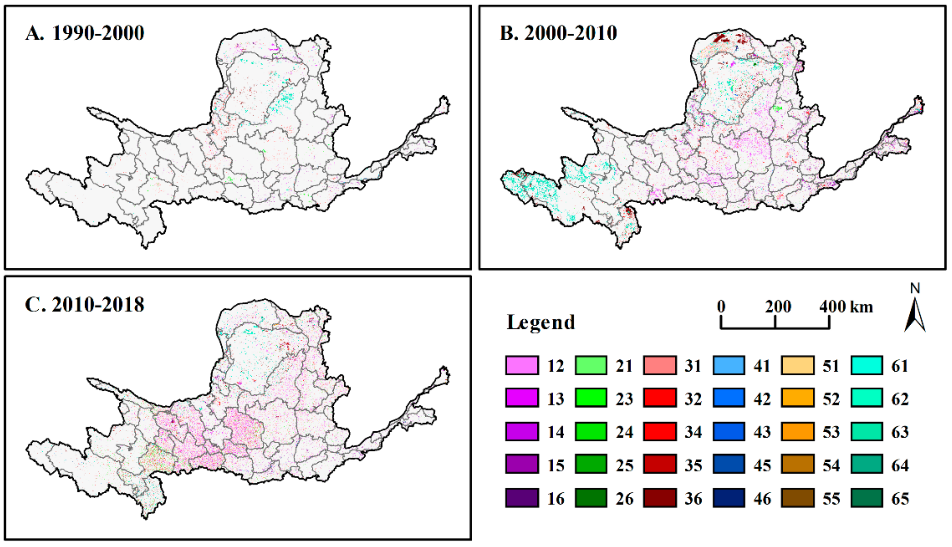
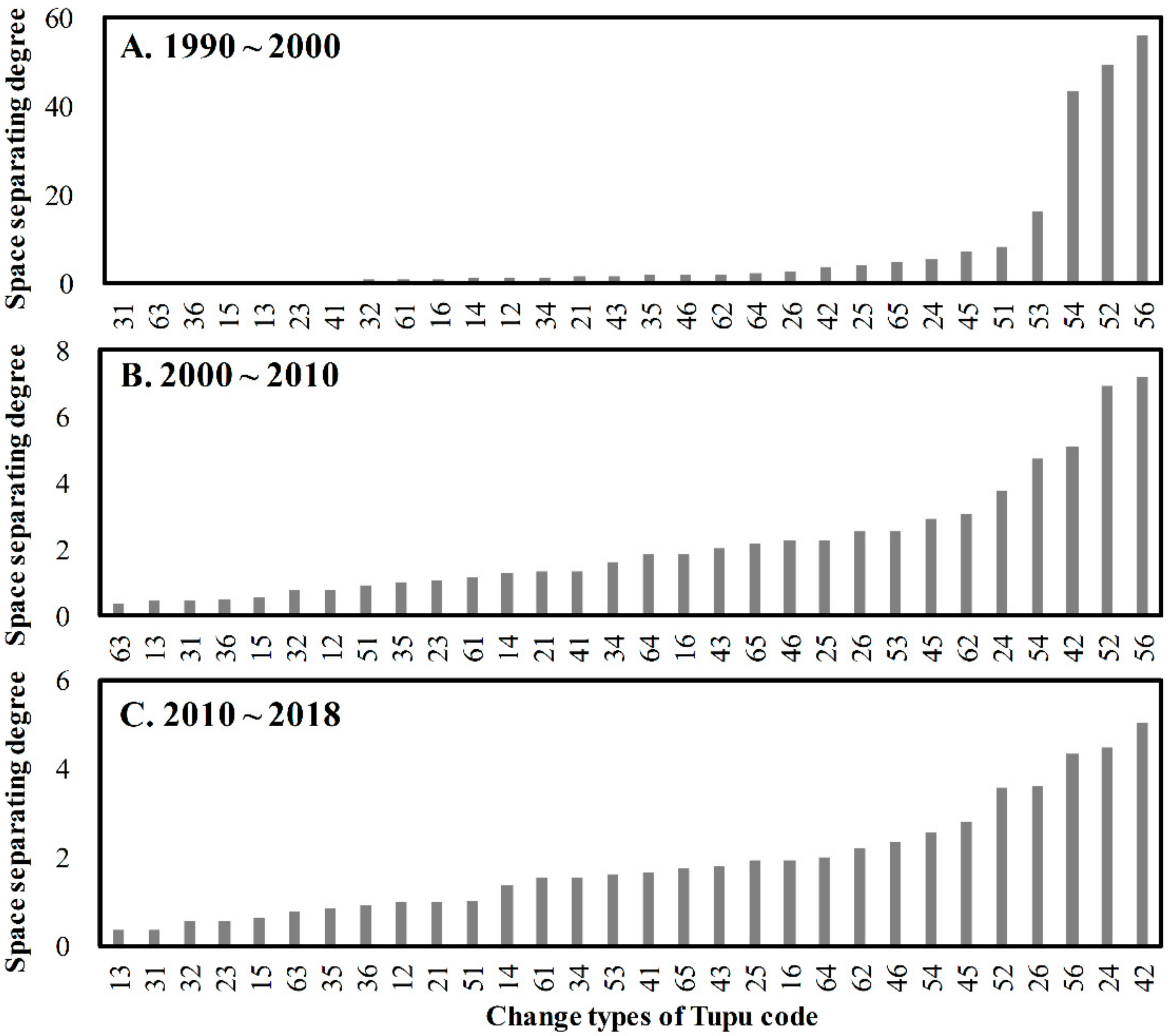
3.2.1. Spatial Distribution of Tupu Units from 1990 to 2018

(1) Spatial distribution of Tupu units from 1990 to 2000

Figure 3A shows the most significant change of Tupu units is “grassland→cultivated land” (31), mainly distributed in the upstream of the YRB. The Tupu units of “unused land→grassland” (63) and “grassland→unused land” (36) were also remarkable, which were widely distributed in the upstream and midstream. The total number of Tupu units of “construction land→cultivated land” (51) was very small, far less than the Tupu units of “cultivated land→construction land” (15), and the spatial distribution of which was relatively scattered.

The spatial separation degree was applied to represent the “Tu” features of the LUT in a quantitative manner. It could reflect the discrete degree of spatial distribution for LUT Tupu units. The higher the spatial separation degree, the greater dispersed the spatial distribution of Tupu units. Based on the spatial separation degree of the LUT Tupu units, we can obtain a visual display of the “Tu” of the LUT, as shown in Figure 4A. The spatial separation degree of Tupu units of Type 31, 63, 36, 15, 13, 23, 41, 32, and 61 were all very low, indicating that these Tupu units were more concentrated in space. Specifically, the spatial separation degree of Tupu units of “grassland→cultivated land” (31) and “unused land→grassland” (63) were 0.33 and 0.43, respectively. Moreover, the spatial distribution of Tupu units of Type 36 (0.56) and 13 (0.58) presented a spatial agglomeration phenomenon. However, the spatial separation degree of Tupu units of “construction land→unused land” was the largest (56.07), followed by the Tupu units of Type 52 and 54 (49.41 and 43.28), indicating that these Tupu units were very dispersed.

(2) Spatial Distribution of Tupu Units from 2000 to 2010

The spatial pattern distribution of Tupu units at this stage showed clustered distribution of some types, as shown in Figure 3B, which were more complicated than the previous stage. The mutual conversions between grassland and cultivated land, and grassland and unused land were still the most significant Tupu units at this stage, which showed a continuous expansion in the midstream and clustered distribution in the upstream. Meanwhile, the mutual transformation between cultivated land and construction land was relatively obvious, “cultivated land→construction land” (15) was mainly distributed in the downstream of the YRB, and also widely distributed in Shanxi, southern Shaanxi, and northwest Yinchuan of Ningxia. While the cultivated land occupation for construction land was relatively dispersed, “construction land→cultivated land” (51) was mainly distributed in the downstream, southern Shanxi, and Bayannaoer of Inner Mongolia. The process of occupying water area for construction land was intensified, and Tupu units of 45 were mainly distributed in Shanxi (Jinzhong, Luliang, and Changzhi), Henan (Luoyang and Zhengzhou), and coastal areas of Shandong.

As shown in Figure 4B, overall separation degree value of this stage was 64.88, which was much smaller than that of the previous stage (222.31), indicating that the spatial pattern of LUT in the YRB was less dispersed. The degrees of spatial separation in Tupu units (codes 63, 13, 31, 36, 15, 32, 12, and 51) were all less than 1, indicating that these Tupu units were intensively distributed in space. The degree of spatial separation of Tupu unit for Type 56 was the highest (7.22), followed by the Tupu units with codes of 52, 42, 54, 24, and 62, indicating that these Tupu units were relatively dispersed. We found that the conversions between construction land and other land use types were scattered throughout the YRB.

(3) Spatial distribution of Tupu units from 2010 to 2018

The most important type of transition was the mutual transformation between cultivated land and grassland, which continued to expand in the midstream of the YRB and gradually developed the cluster distribution in the upstream, as shown in Figure 3C. The interconversion between grassland and forestland changed from scattered distribution to centralized distribution, but the distribution area changed little. The distribution of Type 15 was still relatively concentrated, except in Henan and Shandong, and the same situation also appeared in Gansu (northern Lanzhou). In addition, grassland erosion of forestland and unused land were concentrated, and “forestland→grassland” (23) and “unused land→grassland” (63) were concentrated in Inner Mongolia and Gansu.

The overall separation degree value of Tupu units of LUT was 55.97 during 2010–2018, which was further reduced compared with the previous two stages, as shown in Figure 4C. The spatial separation of Tupu units of Type 13, 31, 32, 23, 15, 63, 35, 36, 12, and 21 were all less than 1. Specifically, spatial separation degrees of Tupu units of Type 13, 31, 32, and 63 were 0.35, 0.37, 0.57, and 0.78, respectively, which were slightly lower than those in the previous stage. However, the spatial separation degrees of Tupu units of Type 15, 36, and 12 were higher than the previous stage. The spatial separation degree of Tupu units for Type 51 increased, indicating that although land reclamation activities are promoted continuously, it is still difficult to make up for the decrease in the total volume. Relatively speaking, Type 15 distribution has a higher spatial concentration, which further verifies that human activities occupy cultivated land violently. The spatial separation degree of Type 42 was the largest and slightly decreased compared with the previous stage. Similarly, the spatial distribution of Tupu units with codes of 56, 26, and 56 were discrete, with the spatial separation degree exceeding 3.

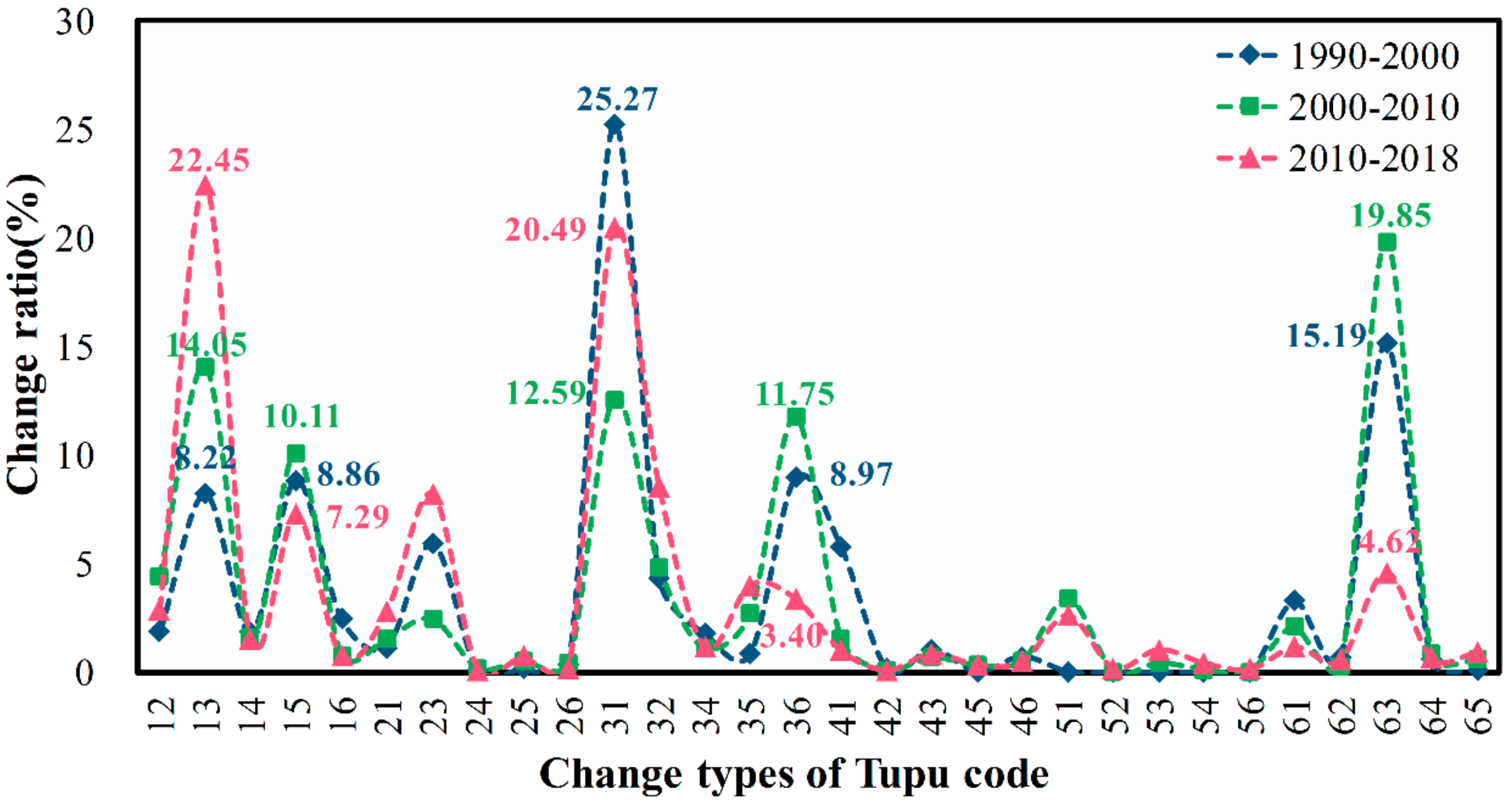
3.2.2. Quantity Change of Tupu Units from 1990 to 2018

The total area of land use change in 1990–2000, 2000–2010, and 2010–2018 was 14,872.17 km², 65,364.84 km², and 64,945.99 km², respectively, as shown in

Table 3. Tupu unit sequence of land use transitions (LUTs) from 1990 to 2018 in the YRB.

Sequence	1990–2000			2000–2010			2010–2018
	Type	Area (km2)	Change Ratio (%)	Type	Area (km2)	Change Ratio (%)	Type	Area (km2)	Change Ratio (%)
1	31	3757.86	25.27	63	12,976.90	19.85	13	14,580.50	22.45
2	63	2258.58	15.19	13	9184.49	14.05	31	13,310.50	20.49
3	36	1333.30	8.97	31	8227.12	12.59	32	5538.27	8.53
4	15	1317.42	8.86	36	7680.71	11.75	23	5345.11	8.23
5	13	1222.70	8.22	15	6606.34	10.11	15	4733.88	7.29
6	23	885.09	5.95	32	3143.63	4.81	63	2998.93	4.62
7	41	861.78	5.79	12	2867.07	4.39	35	2622.12	4.04
8	32	642.81	4.32	51	2229.56	3.41	36	2207.89	3.40
9	61	490.99	3.30	35	1754.52	2.68	12	1886.48	2.90
10	16	365.24	2.46	23	1594.11	2.44	21	1844.11	2.84
11	14	274.22	1.84	61	1380.05	2.11	51	1714.97	2.64
12	12	273.10	1.84	14	1073.97	1.64	14	975.63	1.50
13	34	266.72	1.79	21	1021.60	1.56	61	761.38	1.17
14	21	171.74	1.15	41	1005.42	1.54	34	754.34	1.16
15	43	159.54	1.07	34	710.22	1.09	53	691.23	1.06
16	35	125.18	0.84	64	539.28	0.83	41	662.85	1.02
17	46	108.95	0.73	16	524.79	0.80	65	590.64	0.91
18	62	105.12	0.71	43	433.07	0.66	43	565.57	0.87
19	64	88.25	0.59	65	391.03	0.60	25	482.38	0.74
20	26	55.91	0.38	46	354.19	0.54	16	480.06	0.74
21	42	31.37	0.21	25	353.85	0.54	64	450.09	0.69
22	25	27.60	0.19	26	278.37	0.43	62	368.80	0.57
23	65	19.35	0.13	53	275.65	0.42	46	327.44	0.50
24	24	13.36	0.09	45	216.24	0.33	54	279.56	0.43
25	45	7.86	0.05	62	193.09	0.30	45	233.45	0.36
26	51	6.03	0.04	24	127.59	0.20	52	142.83	0.22
27	53	1.57	0.01	54	80.30	0.12	26	138.99	0.21
28	52	0.17	0.00	42	69.04	0.11	56	96.85	0.15
29	54	0.22	0.00	52	37.84	0.06	24	89.87	0.14
30	56	0.13	0.00	56	34.82	0.05	42	71.28	0.11
Total		14,872.17	100.00		65,364.84	100.00		64,945.99	100.00

Note: No. 1–6 has the same meaning as Figure 3. The Tupu units’ codes can be seen in Table A1.

. During 1990–2000, the change rate of transformation between grassland and cultivated land, and unused land and grassland was 40.46%, which were the main transformation types. In the process of mutual transition between cultivated land and grassland, the area occupied by grassland (3757.86 km²) was much larger than the area supplemented by cultivated land (1222.70 km²). Overall, the accumulative change rate of grassland transfer-out in this stage was 41.19%, which was higher than 30.44% of grassland transfer-in, with a net decrease of grassland quantity. In addition, the scale occupied of cultivated land was also very large, but the area of other land use types transforming into the cultivated land (3452.68 km²) was less than the area of cultivated land they occupy (5288.40 km²). The conversion between construction land and water area, and forestland and unused land was less; the change rate was less than 0.01%.

During 2000–2010, the Tupu unit change rate of Type 63 was 19.85%, which was the most important LUT type and increased 4.66% compared with the previous stage, as shown in Figure 5. Tupu units of 13 rose to second place from fifth place of the previous stage and cultivated land became a grassland transfer-in type, ranking only second to unused land, which was mainly due to the implementation of the policy of returning farmland to grassland. The Tupu unit of 31 and 36 were other important transformation types, accounting for 12.59% and 11.75% of the converted land-use types, respectively. Among grassland transfer-in types, Type 23 (3143.63 km², 4.81%) and 43 (433.07 km², 0.66%) slightly decreased compared with the previous stage, and the number of Tupu units of 13 (9184.49 km², 14.05%), 53 (275.65 km², 0.42%), and 63 (12,976.90 km², 19.85%) all increased to a different extent. The conversion between cultivated land and construction land became increasingly prominent; a total of 6606.34 km² of cultivated land was converted into construction land, while only 2229.56 km² of construction land was converted into cultivated land. The accumulative change rate of cultivated land transfer-out was 30.99%, which was larger than cultivated land transfer-in (21.21%), with a net cultivated land decrease of 6392.91 km².

From 2010 to 2018, mutual transformation between cultivated land and grassland was the main LUT type, with an accumulative change rate of 22.45%. Among these types, the change rate of Type 13 was 22.45%, which increased significantly compared with the previous two stages; Type 31 decreased relative to the stage of 1990–2000, indicating that the quantity of supplementary grassland during 2010–2018 was large. However, the grassland transfer-in area was less than the transfer-out area, and the accumulative change rate of grassland transfer-out (37.62%) was slightly higher than the accumulative change rate of grassland transfer-in (37.23%), with a net decrease of 251.78 km². The problem of cultivated land occupied by construction land was still outstanding, with an area of 4733.88 km². Compared with the previous two stages, the change rate of cultivated land transfer-out increased (34.89%), and transfer-in decreased (28.17%). It was mainly due to the fact that a large amount of cultivated land was occupied by grassland and construction land. Totally, the accumulative change rate of cultivated land transition (CLT) gradually increased, and reached 63.06% from 2010 to 2018, indicating that CLT has gradually become the main type of LUT in the YRB.

3.3. The Impact of LUTs on ESV

3.3.1. Changes in ESV from 1990 to 2018

The total ESV showed a fluctuating trend of decreasing first, increasing later, and then decreasing again—decreasing from 2653.56 × 10⁸ USD in 1990 to 2644.23 × 10⁸ USD in 2000, then increasing to 2665.65 × 10⁸ USD in 2010, and decreasing to 2664.03 × 10⁸ USD in 2018, which was higher than that in the year of 1990, as shown in

Table 4. Changes in total ESV from 1990 to 2018 (×10⁸ USD).

Region	Land Use Types	Codes	ESV in (108 USD)				ESV Change
			1990	2000	2010	2018	1990–2000	2000–2010	2010–2018	1990–2018
Yellow River Basin	Cultivated land	1	459.12	463.01	449.49	440.2	3.89	−13.52	−9.29	−18.92
	Forestland	2	779.57	778.81	800.92	801.63	−0.76	22.11	0.71	22.06
	Grassland	3	1197.47	1192.48	1201.69	1200.65	−4.99	9.21	−1.04	3.18
	Water area	4	190.08	183.02	189.1	197.82	−7.06	6.08	8.72	7.74
	Unused land	6	27.32	26.91	24.45	23.73	−0.41	−2.46	−0.72	−3.59
	Total		2653.56	2644.23	2665.65	2664.03	−9.33	21.42	−1.62	10.47
Upstream	Cultivated land	1	186.65	190.13	189.7	184.94	3.48	−0.43	−4.76	−1.71
	Forestland	2	325.3	323.86	335.91	338.26	−1.44	12.05	2.35	12.96
	Grassland	3	950.38	943.66	952.39	953.1	−6.72	8.73	0.71	2.72
	Water area	4	121.81	122.14	124.66	130.45	0.33	2.52	5.79	8.64
	Unused land	6	24.87	24.97	25.47	21.96	0.1	0.5	−3.51	−2.91
	Total		1609.01	1604.76	1628.13	1628.71	−4.25	23.37	0.58	19.7
Midstream	Cultivated land	1	198.18	198.15	186.4	183.81	−0.03	−11.75	−2.59	−14.37
	Forestland	2	380.94	381.97	393.42	391.85	1.03	11.45	−1.57	10.91
	Grassland	3	227.82	229.92	234.71	232.95	2.1	4.79	−1.76	5.13
	Water area	4	33.19	32.1	29.76	30.12	−1.09	−2.34	0.36	−3.07
	Unused land	6	2.26	1.78	1.79	1.68	−0.48	0.01	−0.11	−0.58
	Total		842.39	843.92	846.08	840.41	1.53	2.16	−5.67	−1.98
Downstream	Cultivated land	1	74.3	74.73	73.39	71.45	0.43	−1.34	−1.94	−2.85
	Forestland	2	73.34	72.98	71.59	71.52	−0.36	−1.39	−0.07	−1.82
	Grassland	3	19.23	18.84	14.59	14.59	−0.39	−4.25	0	−4.64
	Water area	4	34.94	28.64	34.15	36.77	−6.3	5.51	2.62	1.83
	Unused land	6	0.18	0.15	0.05	0.09	−0.03	−0.1	0.04	−0.09
	Total		201.99	195.34	193.77	194.42	−6.65	−1.57	0.65	−7.57

. During the study period, grassland contributed to most of the total ESV (more than 45%), followed by forestland (30%), and unused land contributed the least to the total ESV. The ESV provided by forestland and water decreased during 1990–2000 and increased during the following two periods, while the ESV provided by cultivated land increased during 1990–2000 and decreased during the following two periods. The ESV provided by grassland decreased (−4.99 × 10⁸ USD) during 1990–2000, increased (9.21 × 10⁸ USD) during 2000–2010, and decreased (−1.04 × 10⁸ USD) during 2010–2018. Notably, the ESV provided by unused land was in a decreasing state (−3.59 × 10⁸ USD). Overall, the area of cultivated land decreased, resulting in the ESV’s loss of 18.92 × 10⁸ USD. However, the growth of forestland area in the same period brought an ESV increase of 22.06 × 10⁸ USD, and eventually led to the overall rise of ESV, which verified the effectiveness of the implementation of the policy of returning farmland to forest and a series of protective forest protection plans in the YRB.

The changes in ESV among the upstream, midstream, and downstream showed significant differences, as shown in Table 4. During the study period, the ESV provided by upstream increased (19.7 × 10⁸ USD), and the ESV provided by midstream and downstream decreased (−1.98 × 10⁸ USD, −7.57 × 10⁸ USD). In terms of stages, the ESV of upstream decreased during 1990–2000 (−4.25 × 10⁸ USD), increased greatly during 2000–2010 (23.37 × 10⁸ USD), and then increased slightly during 2010–2018 (0.58 × 10⁸ USD). The ESV of midstream increased during the first two periods and decreased during the following period, while the ESV of downstream showed an opposite tendency. In terms of the proportion of the ESV, the upstream, midstream, and downstream of the YRB were quite different. For upstream, the ESV provided by grassland, forestland, and cultivated land accounted for more than 90%, and the ESV of grassland accounted for 58.52%, which was in a dominant position. The difference between the midstream and the upstream was that the ESV of the forestland accounted for the largest proportion (46.05%); for downstream, cultivated land, forestland, and water area were the three land use types that provide more ESV, of which cultivated land accounted for the largest proportion (36.75%).

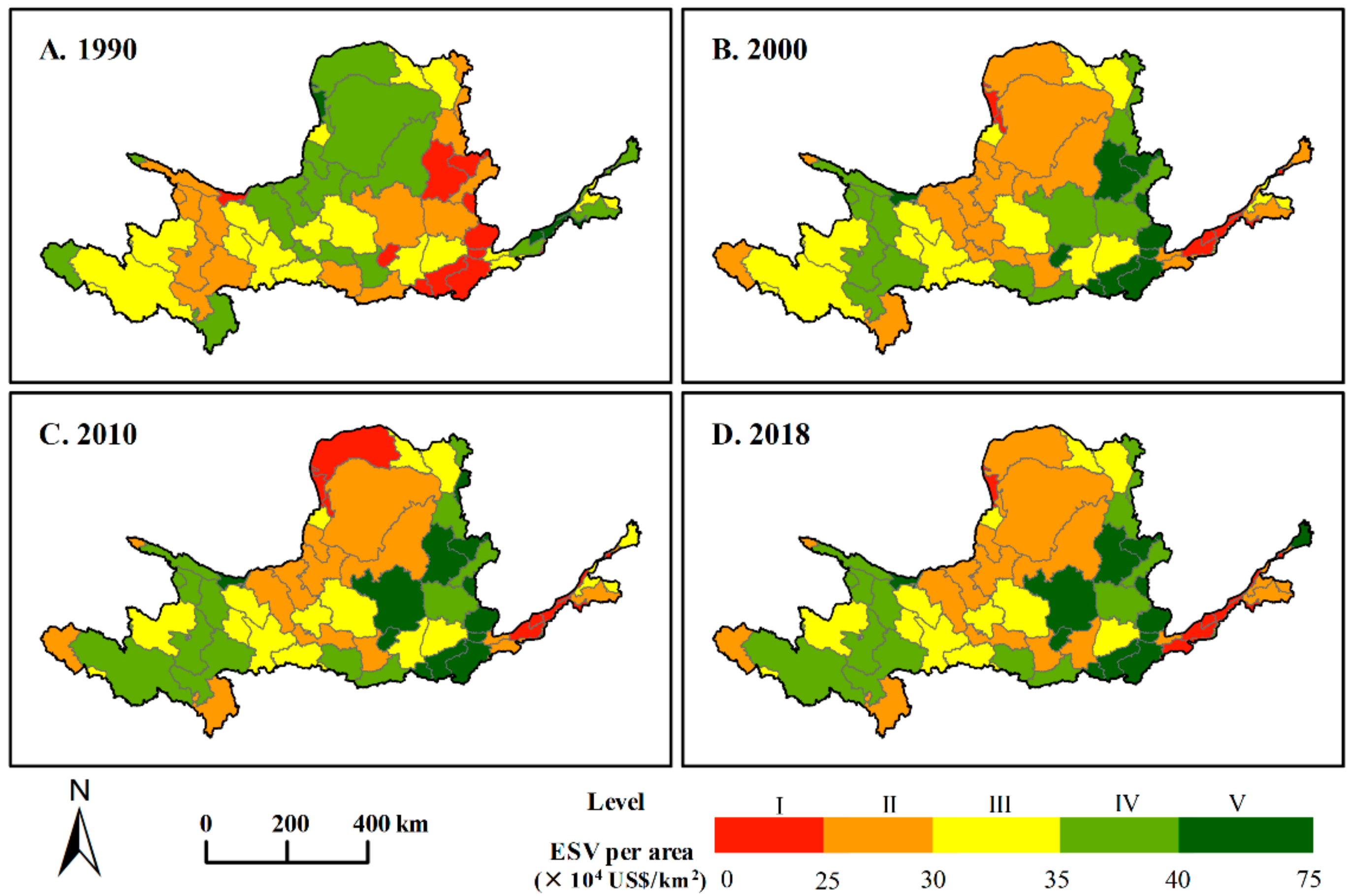
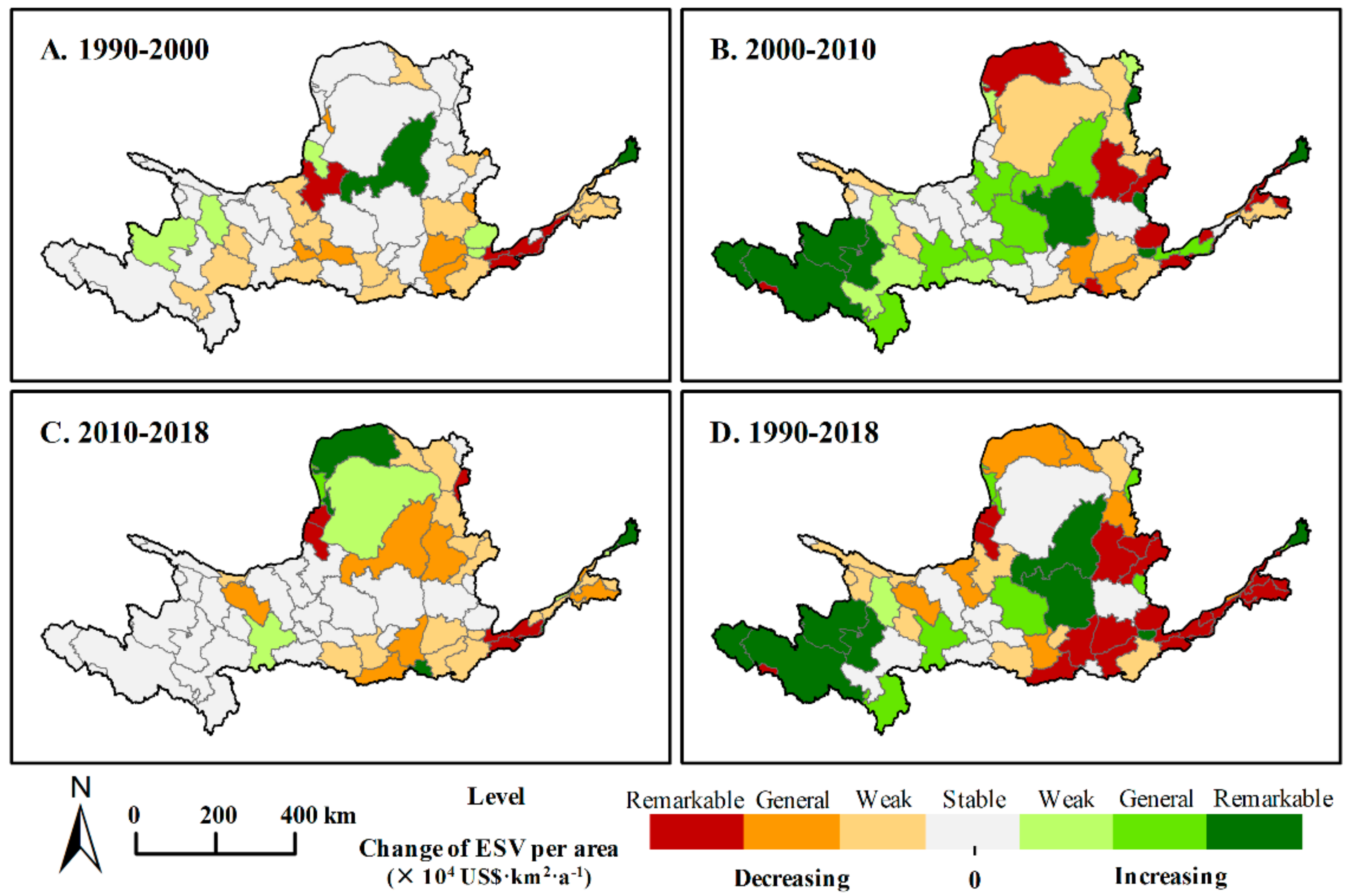
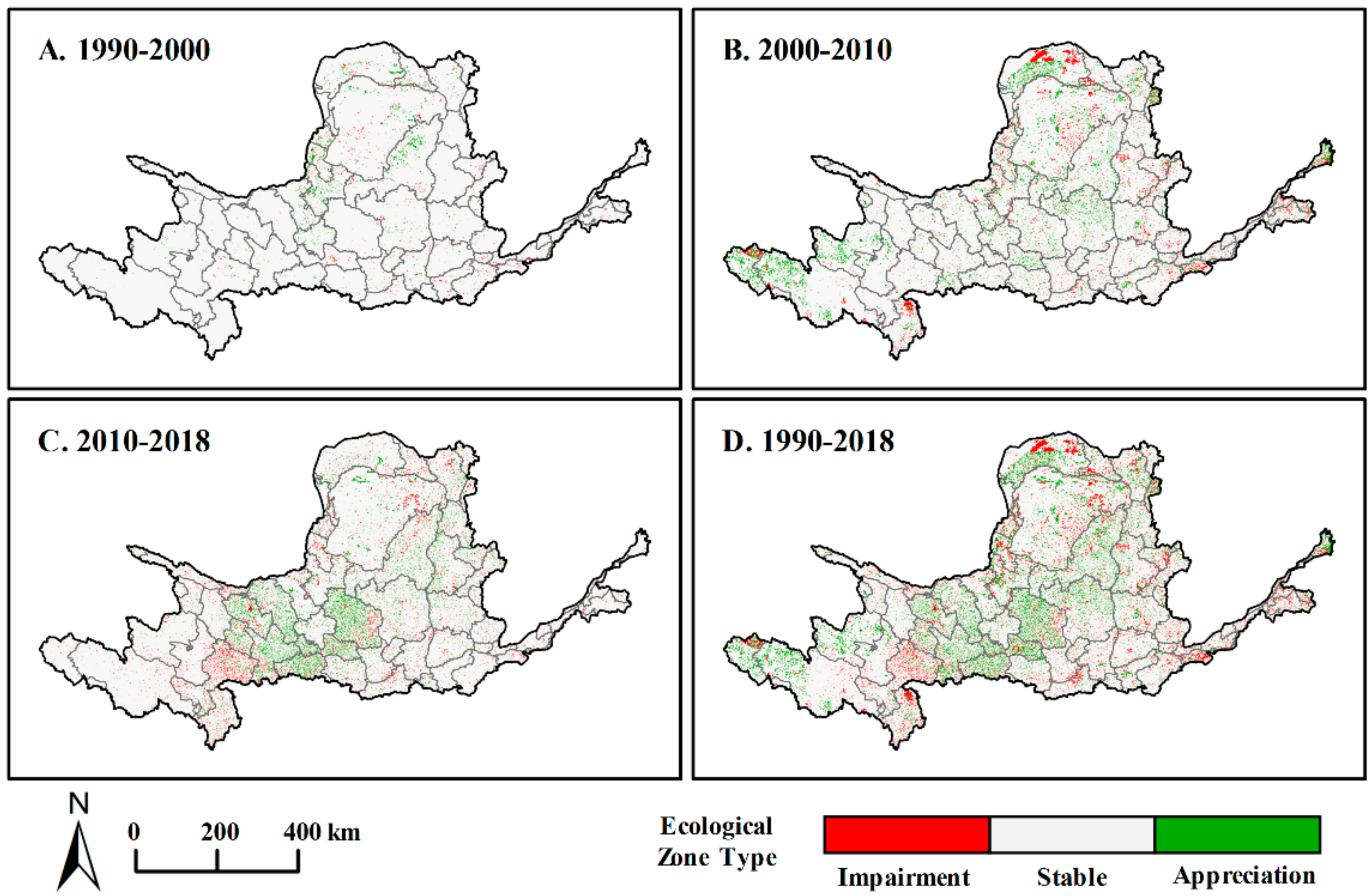
3.3.2. Spatial Distribution of ESV from 1990 to 2018

From 1990 to 2018, the distribution of average ESV (AESV) in the YRB had significant spatial heterogeneity, as shown in Figure 6. Overall, the high-value areas of AESV were mainly distributed in Qinghai, Gansu, central Shaanxi, northern Henan, and Shanxi. These areas were mountainous and hilly, not suitable for farming, forestland and grassland were widely distributed, and the ecological environment was relatively good. The low-value areas were mainly distributed in Ningxia, Inner Mongolia, and eastern Henan and Shandong, mainly due to the distribution of unused land and construction land in these areas, the ecological environment was relatively poor. Specifically, (1) Grade I was mainly distributed in the east of Henan Province (Xinxiang, Anyang, Puyang), and the west of Shandong (Liaocheng, Jining), and the western Inner Mongolia (Alxa League and Wuhai City). In addition, Zhengzhou of Henan and Bayannaoer of Inner Mongolia presented Grade I in 2018 and 2010, respectively. (2) Grade II was distributed in central and southern Ningxia, western Inner Mongolia, western Qinghai, northern Sichuan, and some cities in Gansu. In addition, northern Shaanxi (Yulin) and central Shandong (Jinan, Tai’an) also had distribution. (3) Grade III was mainly distributed in the upstream, including Lanzhou, Tianshui, Dingxi, Qingyang, Hohhot, Baotou, Ningxia, and some cities in Qinghai. (4) Grade IV was mainly distributed in the upstream (Qinghai, Gansu) and the midstream (southern Shaanxi and some cities in Shanxi). (5) Grade V was mainly distributed in the midstream and downstream—the midstream included Luliang, Taiyuan, Changzhi, Jincheng, Yan’an, and Tongchuan in Shaanxi, and the downstream included Luoyang, Sanmenxia, Jiyuan, etc. In addition, Wuwei of Gansu in the upstream was also Grade V. Notably, the AESV in Dongying of Shandong was upgraded from Grade II (1990) to Grade V in 2018.

From 1990 to 2018, the AESV in the YRB changed dramatically, as shown in Figure 7. Specifically, the change degree in 2000–2010 was the most severe, and the whole basin has changed in different degrees and directions. In 2010–2018, the changes were mainly concentrated in the north and southeast of the YRB, and the changes from 1990 to 2000 were relatively scattered. Among them, the AESV in Qinghai increased significantly (2000–2010), Yulin and Yan’an in Shaanxi also increased in 1990–2000 and 2000–2010, respectively. From 1990 to 2018, the AESV of Dongying showed a sustained and obvious upward trend. In addition, the AESV of Ningxia (Yinchuan, Shizuishan) decreased significantly, mainly in 2010–2018. The AESV of Shanxi (Luliang, Taiyang, Jinzhong, Jincheng, etc.) decreased significantly in 2000–2010, while Shaanxi (Xi’an, Weinan) decreased to varying degrees from 1990 to 2018, which led to a significant decrease in the whole study period. The AESV of Henan (Sanmenxia, Yuncheng, Xinxiang, Anyang, Puyang) and central Shandong (Jinan, Jining, Liaocheng, Tai’an) declined significantly. It is worth noting that Bayannaoer in Inner Mongolia decreased significantly from 2000 to 2010, but increased significantly from 2010 to 2018, which led to a general downward trend in the whole study period.

3.3.3. Changes in ESV in Response to LUT

There are two effects of LUT on the ecological environment—improving (positive contribution rate) and reducing (negative contribution rate) ecosystem service functions [55], as shown in

Table 5. Changes in the total ESV in response to LUT in the YRB from 1990 to 2018.

Type	1990–2000		2000–2010		2010–2018		1990–2018
	Changes of ESV (×108 USD)	Contribution Rate (%)	Changes of ESV (×108 USD)	Contribution Rate (%)	Changes of ESV (×108 USD)	Contribution Rate (%)	Changes of ESV (×108 USD)	Contribution Rate (%)
12	1.479	2.943	15.523	7.639	10.213	5.227	22.947	6.374
13	1.234	2.455	9.271	4.563	14.718	7.532	20.550	5.708
14	3.096	6.160	12.124	5.967	11.014	5.637	17.042	4.734
15	−2.787	−5.546	−13.974	−6.877	−10.014	−5.125	−23.900	−6.639
16	−0.637	−1.267	−0.915	−0.450	−0.837	−0.428	−1.287	−0.358
21	−0.930	−1.851	−5.531	−2.722	−9.984	−5.110	−12.370	−3.436
23	−3.899	−7.758	−7.021	−3.455	−23.543	−12.049	−29.065	−8.074
24	0.078	0.156	0.750	0.369	0.528	0.270	1.356	0.377
25	−0.208	−0.414	−2.664	−1.311	−3.632	−1.859	−5.336	−1.482
26	−0.400	−0.796	−1.992	−0.980	−0.995	−0.509	−2.632	−0.731
31	−3.793	−7.547	−8.305	−4.087	−13.436	−6.876	−20.564	−5.712
32	2.831	5.633	13.847	6.815	24.394	12.484	35.481	9.856
34	2.742	5.456	7.301	3.593	7.754	3.968	14.866	4.130
35	−0.391	−0.778	−5.482	−2.698	−8.193	−4.193	−12.519	−3.478
36	−3.670	−7.303	−21.142	−10.405	−6.077	−3.110	−26.487	−7.358
41	−9.728	−19.357	−11.350	−5.586	−7.483	−3.830	−19.829	−5.508
42	−0.184	−0.366	−0.406	−0.200	−0.419	−0.214	−0.661	−0.184
43	−1.640	−3.263	−4.452	−2.191	−5.814	−2.975	−8.331	−2.314
45	−0.105	−0.209	−2.898	−1.426	−3.129	−1.601	−4.994	−1.387
46	−1.420	−2.826	−4.616	−2.272	−4.267	−2.184	−5.824	−1.618
51	0.013	0.026	4.716	2.321	3.628	1.857	5.670	1.575
52	0.001	0.002	0.285	0.140	1.075	0.550	0.585	0.163
53	0.005	0.010	0.861	0.424	2.160	1.105	1.603	0.445
54	0.003	0.006	1.076	0.530	3.747	1.918	2.141	0.595
56	0.000	0.000	0.013	0.006	0.036	0.018	0.018	0.005
61	0.856	1.703	2.406	1.184	1.327	0.679	3.713	1.031
62	0.752	1.496	1.382	0.680	2.640	1.351	4.286	1.191
63	6.217	12.371	35.720	17.579	8.255	4.225	44.918	12.477
64	1.150	2.288	7.028	3.459	5.866	3.002	10.653	2.959
65	−0.007	−0.014	−0.146	−0.072	−0.220	−0.113	−0.366	−0.102

Note: No. 1–6 has the same meaning as Figure 3. The Tupu units’ codes can be seen in Table A1.

. From the perspective of each land use type transfer-out, the biggest ESV loss caused by forestland transfer-out was 48.047 × 10⁸ USD, of which the loss from 2010 to 2018 was as high as 37.626 × 10⁸ USD. Secondly, the ESV loss caused by the transformation of water area into other land use types was 39.639 × 10⁸ USD, of which the losses caused by 2000–2010 and 2010–2018 were 23.722 × 10⁸ USD and 21.112 × 10⁸ USD, respectively. The unused land transfer-out brought the largest increase of ESV, which was 63.204 × 10⁸ USD, followed by the cultivated land transfer-out, which was 35.351 × 10⁸ USD. ESV increase resulting from construction land transfer-out was relatively small (10.017 × 10⁸ USD), which mainly occurred in 2000–2010.

The transition of Type 12, 13, 14, 32, 34, 51, 52, 53, 54, 56, 61, 62, 63, and 64 contributed to the increase in ESV. In terms of improving ecological environment, the transition of Type 63 brought the ESV for the largest increase (44.918 × 10⁸ USD), with the highest contribution rate of 12.477%. This was mainly due to the contribution rate of 12.371% and 17.579%, respectively, from 1990 to 2010. The contribution rate of grassland to forestland was the second (9.856%), of which the contribution rate from 2010 to 2018 was 12.484%. This reflected the transformation and utilization of barren grassland, which made the grassland ecosystem in some areas evolve to a higher level of forestland ecosystem. The third was the conversion of Type 12 and 13, with contribution rates of 6.374% and 5.708%, respectively, all of which occurred from 2000 to 2018. In addition, the transition of Type 14 also had a positive effect on the ecological environment, with a contribution rate of 4.734%, and the contribution rate of the three stages decreased slightly, which was 6.160%, 5.967%, and 5.637%, respectively.

The transition of Type 15, 16, 21, 23, 24, 25, 26, 31, 35, 36, 41, 42, 43, 45, 46, and 65 caused the ESV decline. In terms of ESV loss, the transition of Type 23 caused the largest decline of ESV (29.065 × 10⁸ USD), with a contribution rate of −8.074%, of which the contribution rate from 2010 to 2018 was the highest (−12.049%). The conversion of Type 36 took second place, with a contribution rate of −7.358%, of which the contribution rate from 2000 to 2010 was the highest (−10.405%). The third was the conversion of Type 15, with a contribution rate of −6.639%, and the contribution rates of the three stages were similar, which were −5.546%, −6.877%, −5.125%, respectively. Due to the small transition area, the ESV decline caused by Type 65 was only 0.366 × 10⁸ USD, but the contribution rate of the three stages showed an increasing trend.

Figure 8 shows the spatial distribution of ESV changes in the YRB has significant characteristics during 1990–2018. Ecological appreciation zones were widespread in the YRB, particularly in Qinghai, eastern Gansu, Bayannaoer of Inner Mongolia, and central and northern Shaanxi. Ecological impairment zones were mainly concentrated in Sichuan, southwest Gansu, northern Ningxia, Inner Mongolia, southern Shaanxi, and lower reaches of the YRB. In addition, ecological impairment zones were also scattered in other areas.

The range of ecological appreciation was little in 1990–2000, mainly concentrated in Ningxia, northern Inner Mongolia, and northern Shaanxi. During this period, the scope of ecological impairment was relatively large, mainly distributed in Gansu, Inner Mongolia, central and southern Shaanxi, central Shanxi, Henan, and Shandong. Furthermore, the ESV change in 1990–2000 was more severe than that in 2000–2010. The range of ecological appreciation in Shaanxi was expanded, but the range of ecological impairment was reduced. The range of ecological impairment in Inner Mongolia, Shanxi, Henan, and Shandong Province increased, and the range of ecological impairment in central Shanxi and coastal areas of Shandong tended to expand. At this stage, ecological appreciation zones were also distributed in Qinghai, Gansu, and Sichuan. From 2010 to 2018, the range of ecological appreciation zones decreased, and the range of ecological impairment zones increased. Compared with the first two stages, the ecological appreciation zones were widely distributed in Gansu, and the ecological impairment zones were transferred from east to west of the YRB.

4. Discussion

4.1. Interpretation of LUTs

As an important ecological functional area in China, the land use has changed dramatically in the YRB over the past 30 years [6]. Thereinto, the grassland and cultivated land were found to be the dominant land use types, and the conversions between these two types were also the most frequent. Notably, the grassland area changed by +1598 km² (1990–2000), +2950 km² (2000–2010), and −334 km² (2010–2018), respectively. Grassland increased significantly in 2000–2010, mainly due to the implementation of the Grain-for-Green policy since 2003 [59]. This policy aimed to withdraw the cultivated land that was not suitable for farming and to turn it into grassland. Therefore, the implementation of this policy has greatly increased the area of grassland. It shows that the protection of the ecologically fragile watershed by the project is worth learning from other countries and regions. Grassland area decreased from 2010 to 2018, interestingly, and different scholars have different judgments on the leading factors of such change in this period. Some studies believed that climate change was the primary factor [12], while others think that human activities were the leading factor [60]. It is worth noting that China’s economy developed at a high speed since 2008, with the average annual GDP growth rate at around 10%. There is no doubt that a large number of high-intensity and unreasonable human activities have intensified the LUT, such as extensive urbanization construction, coal mining, and industrial processing [61], which have also caused direct losses of ESV. China’s Central Government was also aware of this problem [8]. On the one hand, China’s economy has begun to shift from rapid development to high-quality development. On the other hand, China has been vigorously promoting the construction of ecological civilization, and has implemented projects such as the protection and restoration of degraded grassland since 2012 [62]. Additionally, the transitions between grassland and unused land, and forestland were also relatively frequent, mainly due to the land exploitation, the Natural Forest Conservation Program, and deforestation [5]. During the study periods, the cultivated land area decreased, while the area of construction land continued to increase. This increase in construction land mainly came from the supplement of cultivated land, while the rural residential land was required to be reclaimed as new cultivated land. This was mainly due to the urban construction land increase vs. rural construction land decrease policy and the cultivated land balance policy [63]. This is the regulation and control policy of cultivated land and construction land with Chinese characteristics, which aims to adjust and utilize the unreasonable, inadequate, and abandoned rural construction land. In this way, it could effectively tap the full potential of existing resources of construction land in urban and rural areas and solve the shortage of construction land in cities and industrial parks. This policy is of great significance to the YRB, which could realize the coordination between economic development and ecological environment protection in the YRB. Additionally, the total area of cultivated land in China is large, but there is little cultivated land per capita and a serious shortage of reserve resources, especially in the YRB. These policies’ implementation could promote new construction land to occupy as less cultivated land as possible, so as to ensure food security of the YRB or even China.

4.2. Changes in ESV of Response to LUTs

The ESV increased by 10.47 × 10⁸ USD with a growth rate of 0.39% during 1990–2018, mainly due to the increase of water area and forestland area. According to the proportion of each ESV, the value of cultivated land, forestland, and grassland accounted for more than 90% of the total value, indicating that these land use types were of great significance to the ecological security of the YRB. Overall, the decline of ESV in the YRB was mainly due to the reduction of cultivated land and unused land area, resulting in 22.51 × 10⁸ USD of ecological value loss in the study area, which should be taken as the object of key protection and restoration. However, the ESV of forestland showed different growth, which reflected the effect of ecological restoration policies, such as returning farmland to forest, natural forest protection plans, and three North Shelterbelt programs [64].

The ESV variation in the YRB showed different features in the upper, middle, and lower reaches. Specifically, cultivated land area had a decreasing trend in the upstream, midstream, and downstream, which had a bad impact on the ecological environment in the YRB. Additionally, it could cause a great loss of the ecological service value in the basin. Meanwhile, the water area in the midstream decreased slightly, which made the loss of ESV in the midstream. The area of water in downstream had increased at a slow speed, and the increase of ESV can hardly offset the loss of ESV caused by other land types. The water area in upstream increased rapidly, especially in 2010–2018. Then, the increase of ESV brought by the increase of water area offset the loss of ESV, which was caused by the decrease of cultivated land and unused land area. Therefore, it could make the ESV in the upstream increase generally and keep the stability of the upstream ecosystem.

In some sense, the impact of LUTs on ESV could be understood from the perspective of land use quantity transfer. However, the change of ESV affected by LUTs also showed obvious spatial differences due to the spatial difference of land use change [5]. Thereinto, the high-value areas of AESV mainly concentrated in the upstream and midstream of the YRB, while the low-value areas mainly concentrated in the downstream areas, which were anti-geographical gradient characteristics with an economic development level. In the upstream of the YRB, ESV in Qinghai, Lanzhou, and Sichuan had high value, but the economic development in these areas was backward and human activities were less. In addition, these areas were mostly located at high altitudes, where the perennial melting water of ice and snow nourished the local grassland [54,55]. On the other hand, global warming also intensified the decline of the snow line [56]. The ESV of Shanxi in the midstream was relatively high. Previously, Shanxi Province was an important energy center in China. However, after 2013, Shanxi began to attach importance to transformation development and ecological environment protection and abandoned the extensive and high-intensity coal industry, thus achieving a high ESV effect at present. This also means that energy development and ecological and environmental protection in the YRB can be paid equal attention to, but the key premise lay in their coordination. From further analysis of the change Tupu of ESV in the YRB from 1990 to 2018, we found that the impairment areas of ecosystem services were mainly concentrated in the middle and lower reaches of the YRB, that is, the ecosystem protection pressure of the midstream and downstream was relatively greater than that of the upstream provinces [65].

Interestingly, the change of ESV in the YRB was also closely related to the positioning of the ecosystem service function in the upper and lower reaches of the YRB. For example, the main reason for the decline of ESV in Henan, Shandong, and other provinces in the lower reaches of the Yellow River was that these provinces have flat terrain, convenient irrigation conditions, and are suitable for farming, and they were mostly located as provinces with high yield, so many grasslands and water areas converted into cultivated land. However, Ningxia, Qinghai, Gansu, and other provinces in the upper reaches of the Yellow River have high terrain and steep slope, and they are mainly responsible for water and soil conservation and other ecological services [66]. In the past 30 years, the areas of grassland and forestland have increased significantly, and their service values have been significantly improved. Therefore, the ecological and functional differences between the upper, middle, and lower reaches of the YRB should be fully considered. To sum up, the ecosystem condition in most areas of the YRB has improved in the past 30 years, and the improvement extent is greater than the deterioration extent, which reflects the effect of the Yellow River Regulation to a certain extent. However, the pressure of ecosystem protection and restoration still exists in the YRB, especially in the areas where ESV declines.

4.3. Policy Implications

The LUT and the change of ESV urgently need more appropriate policy guidance, to better realize the protection and development of the YRB. Combined with our research, the following policy recommendations are suggested.

(1)

Sustainable land management (SLM) claims to minimize the negative impacts of land degradation [67], which otherwise results in the deprivation of human welfare [68]. However, our research found that the unsustainable use of natural resources was still widespread in the YRB. Owing to the YRB existing across several of China’s administrative provinces, it is urgent to break down the administrative districts and to establish strategic and participatory land use planning, including environmental and social impact assessments. In fact, such schemes of SLM are very tough to implement because of the multiple institutional interests from different sectors at different scales. Therefore, it is necessary for China’s Central Government to establish a unified SLM organization for the YRB for the whole basin. One of the main functions of this organization is to perfect land use planning on the scale of the YRB, so as to make the LUT more scientific and reasonable. Moreover, the medium- and long-term governance blueprint of the YRB can be planned with reference to the advanced experience of the Rhine River or other watershed areas [67], which could ensure the sustainability, integrity, and clarity of the governance path.

(2)

In the process of the land use transformation and its management in the YRB, there was an obvious absence in the power of enterprise organizations, social institutions, and the public. On the one hand, these non-governmental organizations have not been well developed, and their strength was still very weak; on the other hand, these social forces lack effective channels to participate. Therefore, the social cooperative governance mechanism is urgent to speed up the establishment and improvement, and let social forces fully participate in the management of the YRB. Additionally, it is necessary to form a situation of social cooperation and co-governance by: (a) clarifying the boundary of responsibility among various social subjects, (b) building an efficient coordination and cooperation mechanism, and (c) establishing a multi-subject governance pattern in the YRB.

(3)

The annual per capita ESV of the YRB is only 628 USD and per capita GDP and ESV in 2018 is 12:1, reflecting that the YRB provided very low ESV per capita. Therefore, it is suggested to introduce measurement evaluation of ESV, and integrate the ecosystem services into the decision-making of land use and ecological protection. As we all know, land use for economic growth is unsustainable, so we must make the environmental value decision of land use. However, China’s current land use planning and land use policies do not fully reflect the concept of sustainable land use. A large number of studies have focused on ecosystem services [3,34,55,69,70,71]; how to integrate ecosystem services into land use and ecological protection decisions has always been the focus of discussion [42,72]. Therefore, taking ESV as a quantitative indicator to measure the ecological effect of land use-related policies is of great significance to promote land use decision-making, urban management, and ecosystem protection.

(4)

The upper, middle, and lower reaches are the ecological center, energy center, and economic center in China, respectively. Therefore, it is necessary to fully consider the differences of the eco-environment in the upper, middle, and lower reaches, and classify the watershed according to the different protection priorities of the region. The main contradiction of its governance lies in how to balance the relationship between development and protection [66]. Thus, we suggest: (a) exploring the ecological compensation mechanism for carrying out land utilization in the YRB; (b) balancing the economic benefit of different areas and the principal part of land utilization in the upstream, midstream, and downstream of the YRB; and (c) coordinating the interesting relationship between economic construction and ecological protection. Internationally, Payment for Watershed Ecosystem Services (PWES) replaces the concept of Watershed Ecosystem Services [36]. Thus, to eliminate the negative impact of land use on the environment, some suggestions was purposed as follows: (a) taking ESV as the foundation for determining the ecological compensation standard; (b) exploring the establishment of an ecological compensation mechanism for different regions and different principal parts of land utilization in the upstream, midstream, and downstream; and (c) weighing the benefit difference brought by different land use types.

(5)

Due to the influence of ecosystem services preference in different land use management types, one or several types of specific ecosystem services were pursued, which could intentionally or unintentionally affect the provision of other ecosystem services [5]. This pattern has led to trade-offs and synergies in ecosystem services [61,73]. Therefore, carrying out in-depth research for the influence that the LUT exerts on ESV can provide decision references for further optimizing land use policies. In order to ensure the coordinated development of ecological, economic, and social benefits in the process of rapid urbanization, measures such as delineating the “three zones and three lines” (three zones—ecological zone, agricultural zone, and urban zone; three lines—permanent basic farmland red line, urban development boundary, and ecological red line) should be promoted [74]. At the same time, it is necessary to strengthen ecological protection and restoration, do more to repair ecological damage, and strive to achieve a good balance between the natural ecosystem and human activities.

4.4. Uncertainties and Challenges for Future Research

This research provided a novel approach, which integrated the geo-information Tupu method with spatial analysis to unravel the effect of LUT on ESV. To some extent, it could make up for the lack of comprehensive quantitative assessment of the ecosystem services of the entire YRB and other deficiencies in the existing research. The results could offer a new perspective into the relationship between land use transition, ecosystem services, and land use management widely recognized for understanding the complex human–ecosystem interactions in ecological topics. Moreover, we improved the previous research by revealing the internal process and geographical pattern of LUTs at a more refined raster data level (30 × 30 m). It can capture more information about LUT than that of 1000 × 1000 m resolution land use raster data [4].

Some deficiencies, however, hinder the study and more efforts can be made to improve. Firstly, this paper used the first-class classification standard to classify the land use in the YRB, and the estimated results are slightly rough. Future work could refine the land use types and improve the accuracy of the estimation results. Secondly, this paper has not studied the factors influencing the change of ESV in the YRB and has ignored the ecological value provided by construction land, which is also the content of research in the future.

5. Conclusions

This work revealed the spatio-temporal pattern of LUT by using the geo-information Tupu method and assessed the change in ESV caused by different Tupu units based on the equivalent factor method. The main conclusions were as follows. (1) The mutual conversions between grassland and unused land, and cultivated land and forestland were the primary Tupu units, which were distributed in the upstream and midstream. The conversion of cultivated land to construction land was also remarkable, being mainly distributed in the lower reaches of the basin. The overall separation degree value became increasingly smaller in these three periods, indicating that these Tupu units were more concentrated in space. The spatial separation degree in the Tupu units between construction land and other land use types was obviously higher than that of other Tupu units, indicating the spatial distribution of construction land transition was relatively scattered. Cultivated land transition has gradually become the main type of LUT in the YRB, with a proportion of 63.06% from 2010 to 2018. (2) The total ESV presented a fluctuated upward tendency (+10.47 × 10⁸ USD), but it was periodic, with grassland (45%) and forestland (30%) contributing the most to the total ESV. ESV presented the watershed characteristics of the upstream region > the midstream region > the downstream region of the economic development level. The ESV of upstream increased, while ESV of midstream and downstream decreased. From the perspective of spatial distribution, the high-value AESV were mainly distributed in Qinghai, Gansu, central Shaanxi, northern Henan, and most areas of Shanxi, while the low-value AESV were mainly distributed in Ningxia, Inner Mongolia, eastern Henan, and Shandong. Among them, the changes in AESV were the most drastic from 2000 to 2010. (3) LUT had a certain impact on quantity variation of ESV, and the impact of land type transfer-in and transfer-out on ESV change was quite different. Tupu units 63 and 32 contributed to most of the increase in the ESV, while Tupu units 23 and 36 contributed to most of the decrease in the ESV during 1990–2018. Additionally, the range of ecological appreciation zones were widely distributed and dispersed, and the range of ecological impairment zones were gradually expanded.

References

1. Schmidt, P.; Morrison, T.H. Watershed management in an urban setting: Process, scale and administration. Land Use Policy 2012, 29, 45–52. [Google Scholar] [CrossRef]
2. Liu, Y.; Bi, J.; Lv, J. Classification of ecosystem services and a reclassification framework of watershed ecosystem services. Resour. Sci. 2019, 41, 1189–1200. [Google Scholar] [CrossRef]
3. Long, H.; Liu, Y.; Hou, X.; Li, T.; Li, Y. Effects of land use transitions due to rapid urbanization on ecosystem services: Implications for urban planning in the new developing area of China. Habitat Int. 2014, 44, 536–544. [Google Scholar] [CrossRef]
4. Lu, X.; Shi, Y.; Chen, C.; Yu, M. Monitoring cropland transition and its impact on ecosystem services value in developed regions of China: A case study of Jiangsu Province. Land Use Policy 2017, 69, 25–40. [Google Scholar] [CrossRef]
5. Chen, W.; Zhao, H.; Li, J.; Zhu, L.; Wang, Z.; Zeng, J. Land use transitions and the associated impacts on ecosystem services in the Middle Reaches of the Yangtze River Economic Belt in China based on the geo-informatic Tupu method. Sci. Total Environ. 2020, 701, 134690. [Google Scholar] [CrossRef] [PubMed]
6. Wang, S.; Liu, J.; Ma, T. Dynamics and changes in spatial patterns of land use in Yellow River Basin, China. Land Use Policy 2010, 27, 313–323. [Google Scholar] [CrossRef]
7. Fang, C. Spatial Organization Pattern and High-Quality Development of Urban Agglomeration in the Yellow River Basin. Econ. Geogr. 2020, 40, 1–8. [Google Scholar] [CrossRef]
8. Lu, D.; Sun, D. Development and management tasks of the Yellow River Basin: A preliminary understanding and suggestion. Acta Geogr. Sin. 2019, 74, 2431–2436. [Google Scholar] [CrossRef]
9. Zhang, W.; Wang, L.; Xiang, F.; Qin, W.; Jiang, W. Vegetation dynamics and the relations with climate change at multiple time scales in the Yangtze River and Yellow River Basin, China. Ecol. Indic. 2020, 10, 105892. [Google Scholar] [CrossRef]
10. Wohlfart, C.; Mack, B.; Liu, G.; Kuenzer, C. Multi-faceted land cover and land use change analyses in the Yellow River Basin based on dense Landsat time series: Exemplary analysis in mining, agriculture, forest, and urban areas. Appl. Geogr. 2017, 85, 73–88. [Google Scholar] [CrossRef]
11. Zhang, B.; Miao, C. Spatiotemporal changes and driving forces of land use in the Yellow River Basin. Resour. Sci. 2020, 42, 460–473. [Google Scholar] [CrossRef]
12. Xu, S.; Yu, Z.; Yang, C.; Ji, X.; Zhang, K. Trends in evapotranspiration and their responses to climate change and vegetation greening over the upper reaches of the Yellow River Basin. Agric. For. Meteorol. 2018, 263, 118–129. [Google Scholar] [CrossRef]
13. Daily, G.C.; Soderqvist, T.; Aniyar, S.; Arrow, K.; Dasgupta, P.; Paul, R. The Value of Nature and the Nature of Value. Science 2000. [Google Scholar] [CrossRef] [PubMed] [Green Version]
14. Perring, M.P.; De Frenne, P.; Baeten, L.; Maes, S.L.; Depauw, L.; Blondeel, H.; Caron, M.M.; Verheyen, K. Global environmental change effects on ecosystems: The importance of land-use legacies. Glob. Chang. Biol. 2016, 22, 1361–1371. [Google Scholar] [CrossRef]
15. Lambin, E.F.; Meyfroidt, P. Land use transitions: Socio-ecological feedback versus socio-economic change. Land Use Policy 2010, 27, 108–118. [Google Scholar] [CrossRef]
16. Long, H.; Li, T. The coupling characteristics and mechanism of farmland and rural housing land transition in China. J. Geogr. Sci. 2012, 22, 548–562. [Google Scholar] [CrossRef]
17. Tsai, Y.; Zia, A.; Koliba, C.; Bucini, G.; Guilbert, J.; Beckage, B. An interactive land use transition agent-based model (ILUTABM): Endogenizing human-environment interactions in the Western Missisquoi Watershed. Land Use Policy 2015, 49, 161–176. [Google Scholar] [CrossRef]
18. Long, H.; Qu, Y. Land use transitions and land management: A mutual feedback perspective. Land Use Policy 2018, 74, 111–120. [Google Scholar] [CrossRef]
19. Liu, J.; Kuang, W.; Zhang, Z.; Xu, X.; Qin, Y.; Ning, J.; Zhou, W.; Zhang, S.; Li, R.; Yan, C.; et al. Spatiotemporal characteristics, patterns, and causes of land-use changes in China since the late 1980s. J. Geogr. Sci. 2014, 24, 195–210. [Google Scholar] [CrossRef]
20. Ning, J.; Liu, J.; Kuang, W.; Xu, X.; Zhang, S.; Yan, C.; Li, R.; Wu, S.; Hu, Y.; Du, G.; et al. Spatio-temporal patterns and characteristics of land-use change in China during 2010–2015. Acta Geogr. Sin. 2018, 28, 547–561. [Google Scholar] [CrossRef] [Green Version]
21. Sun, P.; Xu, Y.; Wang, S. Terrain gradient effect analysis of land use change in poverty area around Beijing and Tianjin. Trans. Chin. Soc. Agric. Eng. 2014, 30, 277–288. [Google Scholar] [CrossRef]
22. Wang, C.; Wang, Y.; Wang, R.; Zheng, P. Modeling and evaluating land-use/land-cover change for urban planning and sustainability: A case study of Dongying city, China. J. Clean Prod. 2018, 172, 1529–1534. [Google Scholar] [CrossRef]
23. Liu, J.; Wang, P.; Li, J.; Xu, J.; Liu, X. An Algorithm for Land-Use Pattern Index and Its Application. Geogr. Geo-Inf. Sci. 2009, 25, 107–109. [Google Scholar]
24. Long, H.; Li, X. Analysis on regional land use transition: A case study in Transect of the Yangtze River. J. Nat. Resour. 2002, 17, 144–149. [Google Scholar]
25. Song, X. Discussion on land use transition research framework. Acta Geogr. Sin. 2017, 72, 471–487. [Google Scholar]
26. Nizalov, D.; Thornsbury, S.; Loveridge, S.; Woods, M.; Zadorozhna, O. Security of property rights and transition in land use. J. Comp. Econ. 2016, 44, 76–91. [Google Scholar] [CrossRef] [Green Version]
27. Liu, Y.; Long, H.; Li, T.; Tu, S. Land use transitions and their effects on water environment in Huang-Huai-Hai Plain, China. Land Use Policy 2015, 47, 293–301. [Google Scholar] [CrossRef]
28. Costanza, R.; Arge, R.; Groot, R.D.; Farberk, S.; Belt, M.V.D. The value of the world’s ecosystem services and natural capital. Nature 1997, 387, 253–260. [Google Scholar] [CrossRef]
29. Costanza, R.; de Groot, R.; Sutton, P.; van der Ploeg, S.; Anderson, S.J.; Kubiszewski, I.; Farber, S.; Turner, R.K. Changes in the global value of ecosystem services. Glob. Environ. Chang. 2014, 26, 152–158. [Google Scholar] [CrossRef]
30. Redford, K.H.; Adams, W.M. Payment for Ecosystem Services and the Challenge of Saving Nature. Conserv. Biol. 2009, 23, 785–787. [Google Scholar] [CrossRef]
31. Gascoigne, W.R.; Hoag, D.; Koontz, L.; Tangen, B.A.; Shaffer, T.L.; Gleason, R.A. Valuing ecosystem and economic services across land-use scenarios in the Prairie Pothole Region of the Dakotas, USA. Ecol. Econ. 2011, 70, 1715–1725. [Google Scholar] [CrossRef]
32. Rounsevell, M.D.A.; Pedroli, B.; Erb, K.; Gramberger, M.; Busck, A.G.; Haberl, H.; Kristensen, S.; Kuemmerle, T.; Lavorel, S.; Lindner, M.; et al. Challenges for land system science. Land Use Policy 2012, 29, 899–910. [Google Scholar] [CrossRef]
33. Foley, J.A. Global Consequences of Land Use. Science 2005, 309, 570–574. [Google Scholar] [CrossRef] [PubMed] [Green Version]
34. Tolessa, T.; Senbeta, F.; Kidane, M. The impact of land use/land cover change on ecosystem services in the central highlands of Ethiopia. Ecosyst. Serv. 2017, 23, 47–54. [Google Scholar] [CrossRef]
35. Song, W.; Deng, X. Land-use/land-cover change and ecosystem service provision in China. Sci. Total Environ. 2017, 576, 705–719. [Google Scholar] [CrossRef]
36. Hauck, J.; Görg, C.; Varjopuro, R.; Ratamäki, O.; Jax, K. Benefits and limitations of the ecosystem services concept in environmental policy and decision making: Some stakeholder perspectives. Environ. Sci. Policy 2013, 25, 13–21. [Google Scholar] [CrossRef]
37. De Groot, R.S.; Alkemade, R.; Braat, L.; Hein, L.; Willemen, L. Challenges in integrating the concept of ecosystem services and values in landscape planning, management and decision making. Ecol. Complex 2010, 7, 260–272. [Google Scholar] [CrossRef]
38. Xie, G.; Zhen, L.; Lu, C.; Xiao, Y.; Chen, C. Expert Knowledge Based Valuation Method of Ecosystem Services in China. J. Nat. Resour. 2008, 23, 911–919. [Google Scholar]
39. Xie, G.; Zhang, C.; Zhang, C.; Xiao, Y.; Lu, C. The value of ecosystem services in China. Resour. Sci. 2015, 37, 1740–1746. [Google Scholar]
40. Chaikaew, P.; Hodges, A.W.; Grunwald, S. Estimating the value of ecosystem services in a mixed-use watershed: A choice experiment approach. Ecosyst. Serv. 2017, 23, 228–237. [Google Scholar] [CrossRef] [Green Version]
41. De Oliveira, V.A.; de Mello, C.R.; Beskow, S.; Viola, M.R.; Srinivasan, R. Modeling the effects of climate change on hydrology and sediment load in a headwater basin in the Brazilian Cerrado biome. Ecol. Eng. 2019, 133, 20–31. [Google Scholar] [CrossRef]
42. Liu, J.; Jin, X.; Xu, W.; Fan, Y.; Ren, J.; Zhang, X.; Zhou, Y. Spatial coupling differentiation and development zoning trade-off of land space utilization efficiency in eastern China. Land Use Policy 2019, 85, 310–327. [Google Scholar] [CrossRef]
43. Wang, G.; Wang, S.; Chen, Z. Land-use /land-cover changes in the Yellow River basin. J. Tsinghua Univ. Sci. Technol. 2004, 44, 1218–1222. [Google Scholar]
44. Jiang, W.; Yuan, L.; Wang, W.; Cao, R.; Zhang, Y.; Shen, W. Spatio-temporal analysis of vegetation variation in the Yellow River Basin. Ecol. Indic. 2015, 51, 117–126. [Google Scholar] [CrossRef]
45. He, Z.; He, J. Remote Sensing on Spatio-temporal Evolution of Vegetation Cover in the Yellow River Basin during 1982—2013. Trans. Chin. Soc. Agric. Mach. 2017, 48, 179–185. [Google Scholar] [CrossRef]
46. Omer, A.; Elagib, N.A.; Zhuguo, M.; Saleem, F.; Mohammed, A. Water scarcity in the Yellow River Basin under future climate change and human activities. Sci. Total Environ. 2020, 749, 141446. [Google Scholar] [CrossRef]
47. Tang, Y.; Tang, Q.; Tian, F.; Zhang, Z.; Liu, G. Responses of natural runoff to recent climatic variations in the Yellow River basin, China. Hydrol. Earth Syst. Sci. 2013, 17, 4471–4480. [Google Scholar] [CrossRef] [Green Version]
48. Liu, J.; Liu, M.; Zhuang, D.; Zhang, Z.; Deng, X. Study on spatial pattern of land-use change in China during 1995—2000. Sci. China Ser. D Earth Sci. 2003, 46, 373–384. [Google Scholar]
49. Liu, J.; Zhang, Z.; Xu, X.; Kuang, W.; Zhou, W.; Zhang, S.; Li, R.; Yan, C.; Yu, D.; Wu, S.; et al. Spatial Patterns and Driving Forces of Land Use Change in China in the Early 21st Century. Acta Geogr. Sin. 2009, 64, 1411–1420. [Google Scholar] [CrossRef]
50. Liao, K. The Discussion and Prospect for Geo-Informatic Tupu. Geo-Inf. Sci. 2002, 3, 14–20. [Google Scholar]
51. Wan, J.; Zhu, G.; Peng, Q. Land Use Information Tupu and Its Application. Geomat. Inf. Sci. Wuhan Univ. 2005, 30, 355–358. [Google Scholar] [CrossRef]
52. Chen, S.; Yue, T.; Li, H. Studies on Geo-Informatic Tupu and its application. Geogr. Res. Aust. 2000, 19, 337–343. [Google Scholar]
53. Ye, Q.; Liu, G.; Lu, Z.; Gong, Z.; Marco, M. Research of TUPU on Land Use/ Land Cover Change Based on GIS. Prog. Geogr. 2002, 21, 349–357. [Google Scholar] [CrossRef]
54. Wang, J.; Shao, J.; Li, Y. Geo-Spectrum Based Analysis of Crop and Forest Land Use Change in the Recent 20 Years in the Three Gorges Reservoir Area. J. Nat. Resour. 2015, 30, 235–247. [Google Scholar] [CrossRef]
55. Gong, W.; Yuan, L. Analysis of Land Use and Its Ecosystem Service Value Change by Graphic Information: A Case Study of Harbin Section of Songhuajiang Watershed. Environ. Technol. 2010, 33, 200–205. [Google Scholar] [CrossRef]
56. Yang, A.; Zhu, L.; Chen, S.; Jin, H.; Xia, X. Geo-informatic spectrum analysis of land use change in the Manas River Basin, China during 1975–2015. Chin. J. Appl. Ecol. 2019, 30, 3863–3874. [Google Scholar]
57. Nahuelhual, L.; Vergara, X.; Kusch, A.; Campos, G.; Droguett, D. Mapping ecosystem services for marine spatial planning: Recreation opportunities in Sub-Antarctic Chile. Mar. Policy 2017, 81, 211–218. [Google Scholar] [CrossRef]
58. Wang, Y.; Dai, E.; Yin, L.; Ma, L. Land use/land cover change and the effects on ecosystem services in the Hengduan Mountain region, China. Ecosyst. Serv. 2018, 34, 55–67. [Google Scholar] [CrossRef]
59. Wang, B.; Yang, Q.; Liu, Z. Effect of conversion of farmland to forest or grassland on soil erosion intensity changes in Yanhe River Basin, Loess Plateau of China. Front. For. China 2009, 4, 68–74. [Google Scholar] [CrossRef]
60. Kong, D.; Miao, C.; Wu, J.; Duan, Q. Impact assessment of climate change and human activities on net runoff in the Yellow River Basin from 1951 to 2012. Ecol. Eng. 2016, 91, 566–573. [Google Scholar] [CrossRef]
61. Haase, D.; Schwarz, N.; Strohbach, M.; Kroll, F.; Seppelt, R. Synergies, Trade-offs, and Losses of Ecosystem Services in Urban Regions: An Integrated Multiscale Framework Applied to the Leipzig-Halle Region, Germany. Ecol. Soc. 2012, 17. [Google Scholar] [CrossRef]
62. Yu, H.; Bian, Z.; Chen, F. Mechanism of Land Ecological Restoration in Mining Area: An Analy-sis based on Land Degradation Neutrality Framework. China Land Sci. 2020, 34, 86–95. [Google Scholar] [CrossRef]
63. Shen, X.; Wang, L.; Wu, C.; Lv, T.; Lu, Z.; Luo, W.; Li, G. Local interests or centralized targets? How China’s local government implements the farmland policy of Requisition–Compensation Balance. Land Use Policy 2017, 67, 716–724. [Google Scholar] [CrossRef]
64. Yang, J.; Xie, B.; Zhang, D. Spatio-temporal variation of water yield and its response to precipitation and land use change in the Yellow River Basin based on InVEST model. Chin. J. Appl. Ecol. 2020, 31, 2731–2739. [Google Scholar] [CrossRef]
65. Liu, G.; Yang, Q.; Huang, J. The Change Characteristics and Influence Factors of Ecosystem Services Valuation of the Yellow River Basin from 2000 to 2015. Environ. Conform. Assess. 2020, 12, 90–97. [Google Scholar] [CrossRef]
66. Yu, H.; Bian, Z.; Mu, S.; Yuan, J.; Chen, F. Effects of Climate Change on Land Cover Change and Vegetation Dynamics in Xinjiang, China. Int. J. Environ. Res. Public Health 2020, 17, 4865. [Google Scholar] [CrossRef] [PubMed]
67. Vogl, A.L.; Bryant, B.P.; Hunink, J.E.; Wolny, S.; Apse, C.; Droogers, P. Valuing investments in sustainable land management in the Upper Tana River basin, Kenya. J. Environ. Manag. 2017, 195, 78–91. [Google Scholar] [CrossRef]
68. Siegmund-Schultze, M.; Ppel, J.K.; Sobral, M.D.C. Unraveling the water and land nexus through inter- and transdisciplinary research: Sustainable land management in a semi-arid watershed in Brazil’s Northeast. Reg. Environ. Chang. 2018, 15, 2005–2017. [Google Scholar] [CrossRef]
69. Song, W.; Deng, X.; Liu, B.; Li, Z.; Jin, G. Impacts of Grain-for-Green and Grain-for-Blue Policies on Valued Ecosystem Services in Shandong Province, China. Adv. Meteorol. 2015, 2015, 1–10. [Google Scholar] [CrossRef] [Green Version]
70. Schirpke, U.; Kohler, M.; Leitinger, G.; Fontana, V.; Tasser, E.; Tappeiner, U. Future impacts of changing land-use and climate on ecosystem services of mountain grassland and their resilience. Ecosyst. Serv. 2017, 26, 79–94. [Google Scholar] [CrossRef]
71. Cao, Y.; Li, G.; Tian, Y.; Fang, X.; Li, Y.; Tan, Y. Linking ecosystem services trade-offs, bundles and hotspot identification with cropland management in the coastal Hangzhou Bay area of China. Land Use Policy. 2020, 97, 104689. [Google Scholar] [CrossRef]
72. Liu, W.; Zhan, J.; Zhao, F.; Yan, H.; Zhang, F.; Wei, X. Impacts of urbanization-induced land-use changes on ecosystem services: A case study of the Pearl River Delta Metropolitan Region, China. Ecol. Indic. 2019, 98, 228–238. [Google Scholar] [CrossRef]
73. Bennett, E.M.; Peterson, G.D.; Gordon, L.J. Understanding relationships among multiple ecosystem services. Ecol. Lett. 2009, 12, 1394–1404. [Google Scholar] [CrossRef] [PubMed]
74. Lian, X. Review on Advanced Practice of Provincial Spatial Planning: Case of a Western, Less Developed Province. Int. Rev. Spat. Plan. Sustain. Dev. 2018, 6, 185–202. [Google Scholar] [CrossRef] [Green Version]
Figure 1. Location of the Yellow River Basin.
Land 09 00514 g001
Figure 2. Land use distribution of the Yellow River Basin (YRB) from 1990 to 2018.
Land 09 00514 g002
Figure 3. Process Tupu of LUTs during 1990–2018 in the YRB. (Note: A, B and C denotes the Tupu of LUTs during 1990–2000, 2000–2010, and 2010–2018, respectively. The No. 1–6 represent cultivated land, forestland, grassland, water area, construction land, and unused land, respectively. The Tupu units’ codes could be seen in Table A1. For example, Code 12 represents cultivated land converted to forestland, and the other codes follow the same rule.)
Land 09 00514 g003
Figure 4. Spatial separation degree of Tupu units from 1990 to 2018 in the YRB. (Note: A, B and C denotes the spatial separation degree of Tupu units during 1990–2000, 2000–2010, and 2010–2018, respectively. No. 1–6 has the same meaning as Figure 3. The Tupu units’ codes can be seen in Table A1).
Land 09 00514 g004
Figure 5. Change ratio of Tupu units from 1990 to 2018 in the YRB. (Note: No. 1–6 has the same meaning as Figure 3. The Tupu units’ codes can be seen in Table A1.)
Land 09 00514 g005
Figure 6. Spatial distribution of average ESV (AESV) in the YRB from 1990 to 2018.
Land 09 00514 g006
Figure 7. Change in spatial distribution of AESV in the YRB from 1990 to 2018.
Land 09 00514 g007
Figure 8. Tupu of changes in ESV from 1990 to 2018 in the YRB.
Land 09 00514 g008